THE EVALUATION OF UNIVERSITY EDUCATIONAL PROCESSES: A QUANTILE REGRESSION APPROACH
C. Davino, D. Vistocco
1. INTRODUCTION
Nowadays, the evaluation of educational processes receives great attention by Universities because of its crucial role in the quality certification. In order to be-come worthy of a certification, Universities must be able to monitor each phase of the educational process and to measure the achieved results (CRUI, 2003). This evaluation can deal both with the efficiency and with the effectiveness of the process (Lockheed e Hanushek, 1994), (Vittadini, 2004), (Aitkin, Longford, 1986), (Hanushek, 1986). The first concept is related to the analysis of costs and benefits deriving from the resources allocated to the educational process while the second concept is based on the comparison between the expected and the ob-tained results deriving from the educational process.
Many statistical contributions have been developed in literature to construct and analyse efficiency and effectiveness indicators (Chiandotto, 2002), (Piccolo 2004), (Gori, Montagni, 1997), (Cozzucoli, Ingrassia, 2005), (Davino, Vistocco, 2007).
This paper aims to investigate on the internal effectiveness, namely the effect of an educational process on the students learning capability. In particular, the effect of personal data and of the student career features on the final degree mark is analysed through quantile regression (Koenker and Basset, 1978). The pro-posed approach allows to focus on the effects that the explanatory variables have on the entire conditional distribution of the dependent variable. The paper is or-ganized as follows: in Section 2 quantile regression is introduced highlighting its main added value with respect to classical regression; in Section 3 an analysis of the final degree marks of University of Macerata (Italy) students is carried out; finally some concluding remarks and further developments are provided.
2. QUANTILE REGRESSION: BASIC NOTATIONS AND INTERPRETATION ISSUES
Quantile regression, as introduced by Koenker and Basset (1978), may be con-sidered as an extension of classical least squares estimation of conditional mean
models to the estimation of a set of conditional quantile functions. The book of Koenker (2005) collects the research results on quantile regression, encompassing models that are linear and nonlinear, parametric and nonparametric and focusing both on the model estimation and on the testing phase. Following only a spot on quantile regression is provided, focusing on the different information the model delivers in case of homogeneous and heterogeneous models.
Quantile regression allows to estimate the conditional quantiles of a response variable (y) distribution as a function of a set X of predictor variables.
Although different functional form can be used, the paper restricts to linear regression models and it uses a semiparametric approach in the sense that no pa-rametric distribution assumputions are required for the error distribution, while an assumption is used in order to specify the functional form of the model.
Quantile regression (QR) can be viewed as an extension of classical LS estima-tion for condiestima-tional quantile funcestima-tions.
The QR model for a given conditional quantile θ follows: ( | ) ( )
Qθ y X =Xβθ (1)
where 0 <θ<1and Qθ(.|.)denotes the conditional quantile function for the θ−th quantile. Denoting with xi the i-th regressor (i=1,..,k), the conditional quantile
( | )i
Qθ y x is the inverse of the conditional cumulative distribution function of the response variable, Fθ−1( | )y x . i
The parameter estimates in QR linear models have the same interpretation as those of any other linear model: they measure the change in the conditional quan-tile of y per unit change of a selected regressor, holding the values of the others regressors constant. Therefore each ( )β θi coefficient of the QR model can be interpreted as the rate of change of the θ−th quantile of the dependent variable distribution per unit change in the value of the i-th regressor:
( ) ( ) i i Qθ β θ ∂ ∂ = y x (2)
As specified above, the model is linear in the parameters and the parameters vary according to the effect of θ−th quantile of the unknown error distribution. Al-though in real applications it could be interesting to focus on selected subset of regression quantiles, it is possible to obtain estimates across the entire interval of quantiles. It is worthwile to highlight that QR estimates for the linear model are interpretable as an ascending sequence of planes that are above an increasing proportion of sample observations with increasing values of the θ−th quantiles (Cade and Noon, 2003). Neverthless, the proportion of observations less than or equal to the θ−th quantile could be in general not exactly equal to θ, as to the simplex linear programming formulation of QR (Koenker, 2005). Moreover QR estimates have to be interpreted for intervals of quantiles, as they break the inter-val [0, 1] into a finite number of smaller, unequal length interinter-vals. The number
and length of these intervals are dependent on the sample size, number of pa-rameters, and distribution of the response variable (Koenker, 2005).
A simple example can be useful in order to describe QR estimates exploiting a graphical interpretation. Starting from three random variables, x~N(10, 1),
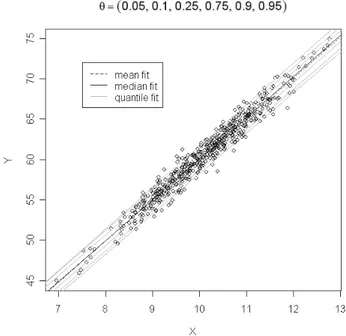
e1~N(µ=0, σ=1) and e2~N(µ=0, σ=1+0.09 x), a sample of n=500 observations is extracted from the modely1=10+5x+e1 (homogeneous error model) and from the model y2=10+5x+e2 (heterogeneous error model). Conditional mean fit, conditionalmedian fit and conditional quantile fits are represented for both the models inFigure 1 and Figure 2, θ = {0.05, 0.1, 0.25, 0.75, 0.9, 0.95}.
For the homogeneous variance regression model (Figure 1), the only estimated effect is a change in central tendency of the distribution of y conditionalon the value of x (location model). Accordingly quantile regression slope estimates are for a common parameter and any deviation among the regression estimates is simply due to sampling variation: an estimate of the rate of change in the mean from ordinary least squares regression is also an estimate of the same parameter as for the quantile regression.
Figure 1 – QR estimates for an homogeneous error model.
When the predictor variable x exerts both a change in mean and a change in variance on the distribution of y (location-scale model), changes in the quantiles of y cannot be the same for all the quantiles. Figure 2 shows that slopeestimates differ across quantiles since the variance in y changes as a function ofx. In such a
case most regression analysis provide an incomplete picture of the relationship between variables, as focusing only on changes in the meansmay misestimate the real changes in the response variable distribution.
Figure 2 – QR estimates for an heterogeneous error model.
The use of quantile regression offers then a more complete view of the rela-tionships among variables, providing a method for modeling the rates of changes in the response variable at multiple points of the distribution. As the independent variables could affect the response variable in different ways at different locations of its conditional distribution, useful insights derive from extracting information at other places other than the expected value. Therefore QR can be used as a complement to standard analysis, allowing a discrimination among cases that would be otherwise judged equivalent using only conditional expectation.
3. AN EMPIRICAL ANALYSIS: THE EVALUATION OF EDUCATIONAL PROCESSES
3.1. The dataset
The aim of the proposed empirical analysis is to evaluate how the student fea-tures affect the outcome of the University careers taking into account that this effect can be different for students with good or bad performances.
QR allows to analyse the dependence of the degree mark from the student fea-tures without restricting to a given location but offering a view on the whole conditional distribution of the dependent variable.
The evaluation of the factors influencing the degree mark is based on a ran-dom sample of 685 students graduated at University of Macerata (Davino, 2007) which is located in the Italian region Marche. The survey has been realized in 2007 and it includes students graduated in the period 2002- 2005.
The following features of the student profile have been observed: gender, place of residence during university education (Macerata and its province, Marche
region, outside Marche), course attendance (no attendance, regular), foreign experience (yes, no), working condition (full time student, working student), number of years to get a degree, diploma mark.
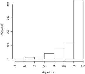
In Figure 3 and in Table 1, the histogram and the main descriptive statistics of the degree mark show an asymmetric distribution: most of the considered students get a degree with a mark greater than 105. Moreover the minimum mark is 77.
Figure 3 – Degree mark distribution.
The characteristics of the degree mark change if the working condition and the numbers of years employed to get a degree are jointly considered (Table 1 and Table 2). Working students get a degree with a mark lower than the full time stu-dents and their marks are highly variable while the 50% of the central votes of full time students ranges from 105 to 110.
As regards to the number of years to get a degree, it results that students graduating in time perfom well and they get a mean mark equal to 107.6 and a median vote equal to 110. On the other side, by increasing the number of years to get a degree, the mean vote reduces and the variability (measured according to interquartile range) raises (Table 1).
TABLE 1
Descriptive statistics of the degree mark
Minimum Q1 Median Mean Q3 Maximum
Total sample 77 102.0 110.0 106.4 110.0 110
Full time student 77 104.8 110.0 106.4 110.0 110
Working students 82 101.0 108.0 104.8 110.0 110
In time graduated 86 107.0 110.0 107.6 110.0 110
Graduated 1 year later 85 106.0 110.0 107.2 110.0 110
Graduated 2 years later 83 101.2 106.0 105.0 110.0 110
Graduated 3 years later 77 98.0 104.0 102.5 110.0 110
Graduated 4 years later 85 97.0 104.0 102.4 110.0 110
TABLE 2
Mean degree mark
Working student Number of years
to get a degree Number of students NO YES
4 179 107.9 107.2 5 156 107.8 106.7 6 158 105.1 104.9 7 101 102.4 102.5 8 49 102.1 102.5 9 42 108.5 100.1
From the analysis of the descriptive statistics, it is possible to gather that the mean degree mark changes on the basis of the student characteristics. Aim of the analysis is to measure the effect (both in strength and in sign) of those features on the final mark by using both classical and quantile regression.
3.2. Main results
The coefficients estimated by LS and QR (the following quantiles are consid-ered: 0.1; 0.25; 0.5; 0.75) are shown in Table 3 (in bold significant coefficients at
α=10%).
Each regression coefficient measures the change of the degree mark deriving from a modification of the corresponding student feature fixing all the others. By performing both the analysis it is possible to gain a detailed description of the factors influencing the whole conditional distribution of the degree mark as LS coefficients measure a change in the conditional mean while QR coefficients measure a change on a given conditional quantile.
From the coefficients in Table 3, it results that the effect of the student fea-tures on the degree mark is different both in sign and in quantity. Gender and residence during university education have a great influence on the lower quan-tiles of the distribution; in particular males and residents outside Marche region show negative coefficients.
A foreign experience positively influences the degree mark but this effect re-duces in the higher part of the distribution pointing that very good students are less influenced by their university experiences.
Working students are less inclined to get high degree marks (LS coefficient is equal to -0.50) but the regression quantile results prove that this effect is relevant in the higher part of the distribution while it is negligible in the lower one.
All the coefficients of the variable “Numbers of years to get a degree” are negative particularly in case of the lower quantiles even if it is worth of notice that only the coefficients related to the quantile 0.25 and 0.5 are significant.
The diploma mark has always a positive effect but its value is very low in case of successful students.
In the higher part of the response variable distribution, the only positive effect is played by regular course attendance while a residence outside Marche nega-tively influence the final degree mark.
TABLE 3
LS and quantile regression coefficients (in bold significant coefficients at α=0.10)
LS β( ).10 β( ).25 β( ).5 β( ).75
(intercept) 96.31 94.94 91.11 97.58 104.56
Gender=Male -2.81 -3.68 -3.65 -3.64 -0.56
Place of residence=outside Marche -3.74 -7.29 -3.81 -4.13 -2.52
Place of residence=Macerata and its province 0.39 1.33 0.52 0.31 0.00
Course attendance=regular 2.65 3.17 3.12 3.04 2.91
Foreign experience=yes 2.18 4.71 2.19 1.38 0.30
Working student=yes -0.50 0.11 0.00 -0.44 -0.30
Number of years to get a degree -0.83 -2.03 -1.35 -0.71 -0.22
Diploma marks 0.15 0.14 0.21 0.13 0.04
In Figure 4, QR coefficients are graphically represented for the different features of the student profile. The horizontal axis displays the different quantiles while the effect of each feature holding constant the others is represented on the vertical axis. The lines parallel to the horizontal axis correspond to LS coefficients, the related confidence intervals are in dashed lines for α=0.1. QR confidence bands (in grey) are obtained through the bootstrap method for α=0.1 (Bilias et al., 2000).
The graphical representation allows to visually catch the different effect of the student characteristics on the degree mark: all the coefficients related to males, place of residence outside Marche and years employed to get a degree are nega-tive even if increasing moving from lower to upper quantiles. On the other hand, place of residence in Marche region, diploma mark and foreign experience play a positive but decreasing effect. Moreover a regular course attendance and working condition have a slighter decreasing effect on the degree mark.
The density estimation of the degree mark can be an useful tool to go into more depth on the effect of a given regressor. Exploiting the quantile regression estimates, indeed, it is straightforward to estimate the degree mark conditional distribution as follows:
ˆ
ˆϑ = β( )θ
y x for 0 < θ < 1
The estimated conditional distribution is strictly dependent on the values used for the covariates. It is then possible to use different potential scenarios in order to evaluate the effect on the conditional degree mark, carrying out a what-if study.
In our analysis, the estimation of the degree mark conditional density is carried out for different values of the numbers of years to get a degree (4, 5, 6, 7, 8, 91) fixing the following conditions for the other regressors: female, place of residence in Macerata, regular course attendance and lowest diploma mark. The obtained densities are shown in Figure 5 along with the quartiles (vertical segments).
The number of years spent at University seems to have an effect on the con- ditional distribution of the degree mark, main pattern being the shift of the first quartile moving from regular to slower students.
Figure 5 – Histograms of the conditional distribution of the final mark (sex=female, place of
resi-dence=Macerata, course attendance=regular, diploma mark=lowest) by number of years to get a degree.
The previously described effect on the first quartile is more evident from the boxplot representation of the conditional densities (Figure 6).
Figure 6 – Boxplots of the conditional distribution of the final mark (sex=female, place of residence=
Macerata, course attendance=regular, diploma mark=lowest) by number of years to get a degree.
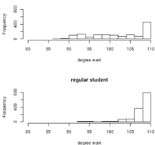
An analogous analysis is conducted in order to evaluate the effect of the work-ing condition on final mark (Figure 7). The densities have been conditioned for working students (Figure 7a) on the group of males, place of residence outside Marche, no course attendance, lowest diploma mark while for full time students (Figure 7b) on males, place of residence in Macerata, regular course attendance, highest diploma mark. The degree mark tends to show higher variability and ex-treme low values in the group of working students.
Figure 7 – Histograms of the conditional distribution of the final mark for working students (sex=
male, place of residence=outside Marche, course attendance=no, diploma mark=lowest) and for regular students (sex=female, place of residence=Macerata, course attendance=regular, diploma mark=highest).
The impact of the student features on the final degree mark can vary in the dif-ferent faculties of University of Macerata. The descriptive statistics of the degree marks (Table 4) and the LS estimations (Table 5) for each Faculty show some critical items:
- gender has a positive influence only in case of students from the Faculty of Communication Science;
- a place of residence outside Marche has a positive influence only in case of students from the Faculties of Communication Science and of Political Sci-ence;
- a regular course attendance greatly influence the final performance of the stu-dents from the Faculties of Economics and Law;
- a foreign experience such as Erasmus exercises a negative influence only in case of students from the Faculty of Communication Science;
- working students in the Faculties of Communication Science and Economic achieve better performances than full time students.
It is worthwile to point out that the interpretation of coefficients in Table 5 must take into account that the results related to the Faculties of Letters and Phi-losophy, Communication Science and Educational Science are conditioned from a median equal to 110.
TABLE 4
Descriptive statistics of the degree marks by Faculty
Minimum Q1 Median Mean Q3 Maximum
Economics 85 98.0 103.0 102.6 110.0 110
Law 77 95.0 102.0 100.6 107.0 110
Letters and Philosophy 94 107.5 110.0 108.0 110.0 110
Communication Science 96 106.5 110.0 107.8 110.0 110
Educational Science 94 108.0 110.0 108.6 110.0 110
Political Science 90 102.0 105.0 104.6 110.0 110
TABLE 5
LS estimations by Faculty (in bold significant coefficients at α=0.10)
Economics Law Letters and Philosophy Communication Science Educational Science Political Science
(constant) 90.97 91.01 101.07 91.47 100.1 105.25
Gender=Male -1.85 -2.86 -0.33 1.13 -2.14 -0.29
Place of residence=outside Marche 1.91 -5.54 -1.49 1.14 -2.04 2.13
Place of residence=Macerata
and its province 0.73 0.13 -0.16 0.18 0.35 0.37
Course attendance=regular 2.15 1.88 0.22 0.30 0.95 1.14
Foreign experience=yes 2.23 2.65 1.48 -0.31 1.63 0.88
Working student=yes 1.63 -1.38 -0.01 1.45 0.37 -1.95
Number of years employed to
get a degree -0.86 -0.63 -0.36 -0.13 0.06 -1.19
4. CONCLUDING REMARKS
Quantile regression represents an useful tool to evaluate the effects of the stu-dent features on the final degree mark distribution. Through the estimation of the degree mark conditional distribution it is also possible to carry out a what-if analysis and to measure the gain it is possible to obtain by modifying the covari-ates.
The proposed approach easily applies to comparisons among educational processes and it provides basic tools to understand results. Some more detailed graphical tools able to summarize the whole information from quantile regression are desirable so to capitalize the whole quantile regression results.
Further developments could include the analysis of the efficiency of a process by comparing costs and benefits deriving from the resources allocated to the edu-cational process. Moreover the use of a multilevel approach (Gelman and Hill, 2006) could be explored in order to use a qualitative variable to separate changes among different levels.
Dipartimento di Studi sullo sviluppo economico CRISTINA DAVINO University of Macerata
Dipartimento di Scienze Economiche DOMENICO VISTOCCO University of Cassino
ACKNOWLEDGEMENTS
Authors wish to thank anonymous referees for helpful comments and suggestions on a previous draft of the paper: they helped to improve the final version of the work.
This research is financially supported by University of Macerata grant “Metodi Stati- stici per la valutazione dell'impatto degli interventi degli organi universitari” (C. Davino). Research work of Domenico Vistocco is supported by Laboratorio di Calcolo ed Analisi Quantitative, Dipartimento di Scienze Economiche, Università di Cassino.
REFERENCES
M. AITKIN, N. LONGFORD,(1986), Statistical Modelling Issues in school Effectiveness Studies,
Journal of the Royal Statistical Society, A 149.
Y. BILIAS, S. CHEN, Z. YING,(2000)Simple resampling methods for censored regression
quan-tiles, Journal of Econometrics, 99, 373-386.
B. CHIANDOTTO, (2002), Valutazione dei processi formativi: cosa, come e perché, in M.R. D’Esposito
(a cura di) “Atti della Giornata di Studio Valutazione della didattica e dei Servizi nel si- stema Università”, Fisciano, 31 maggio 2002.
P. COZZUCOLI, S. INGRASSIA, (2005), Indicatori dinamici di efficienza didattica dei corsi di laurea
uni-versitari, in “Atti della Riunione Scientifica Valutazione e Customer Satisfaction per la qualità dei servizi”, Roma, 8-9 Settembre 2005.
B.S. CADE, B.R. NOON (2003), A gentle introduction to quantile regression for ecologists, “Frontiers in
CRUI, (2003), Guida alla valutazione dei corsi di studio, CampusOne.
C. DAVINO, (2007), Analisi degli sbocchi occupazionali dei laureati dell’Università di Macerata, Eum
(Edizioni Università di Macerata).
C. DAVINO, D. VISTOCCO (2007), La regressione quantile per la valutazione dell’efficacia didattica dei
corsi di studio universitari, in Atti della Riunione Scientifica “Valutazione e Customer Sat-isfaction per la Qualità dei Servizi”, Roma, 12-13 Aprile 2007, Facoltà di Economia, Università degli Studi di Roma Tor Vergata.
E. EIDE, M.H. SHOWALTER (1998), The effect of school quality on student performance: a quantile
regres-sion approach, “Economics Letters”, 58, pp. 345-350.
A. GELMAN, J. HILL(2006), Data analysis using regression and multilevel/hierarchical models,
Cam-bridge University Press.
E. GORI, G. VITTADINI (1999), Qualità e valutazione nei servizi di pubblica utilità, Etas, Milano. E. GORI, M. MONTAGNI (1997), Random effects models for event data-evaluating
effective-ness of university through the analysis of students careers, Multilevel Modelling Newsletter, vol. 10, no. 1, ERC, England.
E.R. HANUSHEK, (1986), The Economics of Schooling: Production and Efficiency in the
Public Schools, Journal of Economic Literature, 24, pp. 1141-1177.
R. KOENKER, G.W. BASSET (1978), Regression Quantiles, “Econometrica”, 46, pp. 33-50. R. KOENKER (2005), Quantile Regression, Econometric Society Monographs.
M.E. LOCKHEED, E.R. HANUSHEK (1994), Concepts of Educational Efficiency and Effectiveness,
Inter-national Encyclopedia of Education, Second Edition.
D. PICCOLO (2004), Un prototipo statistico per la valutazione comparata dell’efficacia didattica dei corsi
di studio universitari, Quaderni di Statistica, 6, pp. 159-186.
G. VITTADINI (2004), Linee guida per la valutazione dell’efficienza esterna della didattica mediante il
Capitale Umano, in E. A. Cutillo (a cura di) Atti del Workshop “Strategie metodologiche per lo studio della transizione Univ.-Lavoro”, CLEUP.
SUMMARY
The evaluation of University educational processes: a quantile regression approach
The paper aims to analyse the internal effectiveness of an university educational proc-ess by means of quantile regrproc-ession. In particular, the goal is to evaluate how the students features affect the outcome of the University careers taking into account that this effect can be different for students with good or bad performances.