A
NALYSIS OF THE VIBRATION LOCALIZATION PHAENOMENON IN IMPERFECT RINGSP. Bisegnaa, G. Carusob∗
aUniversit`a di Roma Tor Vergata - Dipartimento di Ingegneria Civile, 00133 Roma bITC-CNR, 00155 Roma
Sommario
In questo lavoro si considera l’analisi modale di anelli imperfetti che vibrano elasticamente nel proprio piano. Le imperfezioni sono trattate come delle perturbazioni, dipendenti dalla variabile angolare, della densit`a e della rigidezza flessionale dell’anello. Si utilizza la teoria di Eulero Bernoulli per modellare il comportamento dinamico dell’anello imperfetto, e le frequenze e i modi di vibrazione sono ricavati perturbando al primo ordine le frequenze e i modi propri dell’anello perfetto. Infine si considerano alcuni esempi pratici al fine di confrontare i risultati ottenuti con il modello proposto con risultati analoghi ottenuti utilizzando un modello agli elementi finiti.
Abstract
The modal analysis of imperfect rings vibrating in their own plane is considered in this paper. The imperfections are modeled as generic perturbations, depending on the angular variable, of the linear mass density and the bending stiffness of the ring. The Euler-Bernoulli theory is used to develop the dynamical model of the ring, and a perturbation expansion of the solution is performed in order to find out the modal split eigenfrequencies and the relevant perturbed modal shapes. Finally, some case-study problems are considered and the analytical results obtained by using the proposed approach are compared to results obtained by employing a finite-element model of the imperfect ring.
Key words: Imperfect rings, frequency split, localization of vibrations, perturbation expansion
1. INTRODUCTION
Axisymmetric structures are commonly used in practical applications, as turbine bladed disks, satellite antennae, bells, stator-rotor assemblies in electrical machinery, vibrating ring gyroscopes and so on. Due to the periodicity they possess, these structures exhibit degenerate pairs of eigenmodes at the same frequency with modal shapes having sinusoidal behavior with respect to the angular variable. It is well known that when structural irregularities are present, destroying the symmetry of the structure, the pairs of eigenfrequencies coincident in the perfect symmetric case split into two different values. In many cases, like for vibrating ring gyroscopes [1, 2] where a strong resonant coupling between two modes is
required, the frequency split is a drawback effect and must be reduced with a correction procedure called trimming. Moreover, the eigenmodes of a symmetric structure with imperfections deviate from the sinusoidal shape presenting a local increase of vibration amplitude, leading consequently to an increase of the dynamical load on the vibrating structure. This phenomenon is called localization of vibration and may lead to fatigue failure [3, 4]. For these reasons, it is useful to have simple dynamical models able to take into account the presence of imperfection and to predict the frequencies split and localization phenomenon in axisymmetric structures with imperfections.
In this paper the attention is focused on the vibrations of imperfect rings. Many papers can be found in the literature dealing with a quantitative analysis of the frequency split occurring in these structures, and an updated review can be found in [5, 6]. Many causes of imperfections have been considered by researchers and will be briefly summarized in what follows. In [7] a ring with variable cross section has been considered, and the Rayleigh-Ritz method was used to find out the frequency split; a closed form expression for the lower natural frequency was obtained using a first-order approximation. In [5] a simple model for the frequency split of slightly imperfect rings has been developed, based on the Rayleigh-Ritz method together with the simplifying assumption that the eigenmodes of the imperfect ring are still sinusoidal. The imperfections are considered as added masses and radial and torsional springs. Closed form expressions for all the eigenfrequencies of the imperfect ring are obtained; an extension to the case of a distributed mass added to the ring has been proposed in [8], and a study on the statistics of frequency splitting under various added random mass distributions was performed. In [6] in-plane profile variations are taken into account as a cause of frequency splitting. In [9] the frequency split is caused by anisotropy of the material (crystalline silicon) comprising the ring, yielding a dependence of the Young modulus on the angular variable. According to the literature, while a great effort has been spent for the evaluation of the frequency split in imperfect ring, less attention has been devoted to the analysis of the modal shapes of a imperfect ring.
In this paper a theory for the modal analysis of slightly imperfect rings is proposed, yielding closed form expressions for both the frequencies and the modal shapes of the ring. Quite general conditions of imperfection are considered, by assuming that both the linear density and the in-plane bending stiff-ness of the ring are given by the sum of a small perturbation depending on the angular variable and a constant value relevant to the perfect ring. The Euler-Bernoulli theory is adopted to build a dynamical model of the structure, under the assumption that the ring is axially undeformable. A first order perturba-tion expansion of the soluperturba-tion if performed, by assuming that each eigenmode of the imperfect structure can be represented as the sum of an unknown perturbation depending on the angular variable and the corresponding sinusoidal eigenmode relevant to the perfect structure. A non homogeneous partial differ-ential equation is derived, assuming as an unknown function the modal perturbation, and its solvability conditions yield the values of the frequency splits and the corresponding phase angles. Closed-form expressions are obtained for the Fourier series coefficients of the unknown modal perturbation. Finally, some case study problems are considered; the frequency splits and perturbed modal shapes obtained by using the proposed model are compared with the ones obtained via the use of a suitable finite-element formulation.
2. DYNAMICAL MODEL OF A RING
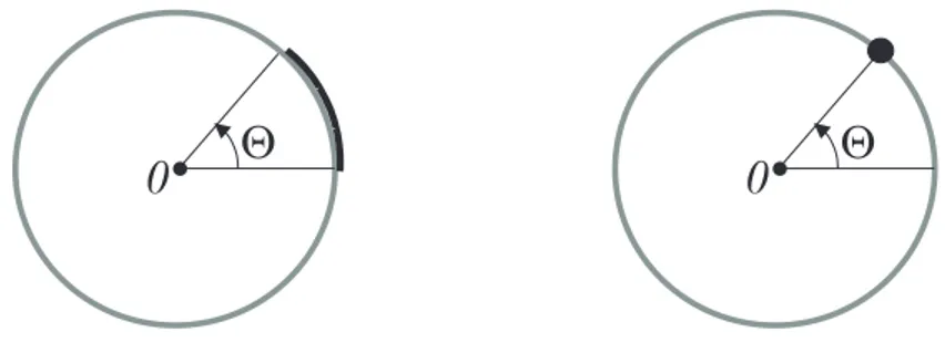
A model of the dynamical behavior of a ring is here derived, based on the classical Euler-Bernoulli theory. The ring of radius R is made of a elastic material. It is here assumed that, due to the presence of imperfections, the linear density σ and the in-plane bending stiffness EI of the ring are functions of the angular variable θ. Let u and v denote, respectively, the tangential and radial displacement as shown in fig. 1. Moreover it is considered that the ring is axially inextensible, i.e. the tangential strain ε is zero.
Figura 1: Schematic representation of the ring
Accordingly the following expression holds:
ε = 1 R µ ∂u ∂θ + w ¶ = 0 (1)
The Hamiltonian functional H for the ring can be written as
H = 1 2 Z t 0 Z 2π 0 σ(θ) "µ ∂u ∂t ¶2 + µ −∂ 2u ∂θ∂t ¶2# R dθdt −1 2 Z t 0 Z 2π 0 E(θ)I(θ) R4 · ∂u ∂θ + ∂3u ∂θ3 ¸2 R dθdt (2) The stationarity condition of (2) gives the dynamic equilibrium equation of the ring, and reads as follows:
∂2 ∂t2 · σu − ∂ ∂θ µ σ∂u ∂θ ¶¸ R − µ ∂ ∂θ + ∂3 ∂θ3 ¶ · EI R3 µ ∂u ∂θ + ∂3u ∂θ3 ¶¸ = 0 (3) 2.1 Perfect ring
If the ring is perfect σ and EI are not depending on θ and are here denoted by σo and EIo. The stationarity condition of H reported in (3) can be simplified into:
σ µ ∂2u ∂t2 − ∂4u ∂θ2∂t2 ¶ − EI R3 µ ∂2u ∂θ2 + 2 ∂4u ∂θ4 + ∂6u ∂θ6 ¶ = 0 (4)
A solution of (4) can be found as:
u = ∞ X n=0 uon= ∞ X n=0 Un cos(nθ + ϕn)e(iωont) (5)
where uonis the eigemnode of circular frequency ωon, nodal diameter n and phase angle ϕn. Substituting
(5) in (4) the following well-known relation between n and ωoncan be found:
ωon2 = EIo σoR4
n2(1 − n2)2
1 + n2 (6)
The eigenmodes relevant to n = 0 and n = 1 corresponds to rigid motions, and thus have frequency equal to 0. All the eigenmodes with k > 0 are degenerate, i.e. two orthogonal eigenmodes exist at the same eigenfrequency.
3. MODAL FREQUENCIES AND MODAL SHAPES EVALUATION
It is well understood that when small imperfections are added to a perfect ring, thus destroying the rotational periodicity of the structure, the frequencies relevant to couples of degenerate eigenmodes, co-inciding when the ring is perfect, split in two different values. Moreover the modal shape of these couples of modes deviates from the sinusoidal shape, exhibiting localized increase of vibration amplitude. In this section a model is established leading to analytical expressions of the frequency splits and the modal shapes of imperfect rings for very general imperfections.
3.1 Position of the problem
In order to take into account the presence of imperfections in a ring, it is assumed that the density σ and the in-plane bending stiffness EI of the imperfect ring are given by:
σ = σo+ δσ(θ), EI = EIo+ δEI(θ) (7)
where σo and EIo are constant values corresponding, respectively, to the density and bending stiffness
of the perfect ring whereas δσ and δEI are small perturbations depending on θ. Accordingly, the eigen-modes unof the imperfect ring can be obtained by perturbing the perfect ring eigenmodes given in (5).
To this end, it is assumed that
un= (uon+ δun)ei(ωon+δωn)t (8)
where δunis a small unknown perturbation of the modal shape uonof the perfect ring, depending on θ and δωnis the unknown perturbation of the corresponding modal circular frequency ωon. A differential
equation for δun can be obtained by substituting the assumptions (7) and (8) in the equation (3). By
remembering that the zero-order terms satisfy the equation (4) and neglecting infinitesimal terms of order higher than 1, the following differential equation is obtained:
−ωon2 σoR µ δun−∂ 2δu n ∂θ2 ¶ −EIo R3 µ ∂2δu n ∂θ2 + 2 ∂4δu n ∂θ4 + ∂6δu n δθ6 ¶ = + ω2onR · δσ uon− ∂θ∂ µ δσ∂uon ∂θ ¶¸ + 2ωonσoR δωn µ uon−∂ 2u on ∂θ2 ¶ + µ ∂ ∂θ + ∂3 ∂θ3 ¶ · δEI R3 µ ∂uon ∂θ + ∂3u on ∂θ3 ¶¸ = 0 (9)
A condition for the existence of a solution of equation (9) is that the non homogeneous term at the right hand side of the equation is orthogonal to the kernel of the self adjoint operator at the left hand side. It can be easily seen that a basis of such a kernel is given by
n
cos(nθ), sin(nθ) o
(10) Accordingly the right end side F (θ) of equation (9) must satisfy
Z 2π 0 F (θ) cos(nθ) = 0, Z 2π 0 F (θ) sin(nθ) = 0 (11)
These two conditions are non linear equations in the scalar the unknowns δωn and ϕn, which can be
for each n ≥ 2 (elastic modes) there are two solutions of system (11), corresponding to the two split fre-quencies δωn1,2of the degenerate pair of eigenmodes relevant to the perfect ring, and the corresponding
two phase angles ϕn1,2. A weak version of (9) is given by: Z 2π 0 · −ω2onσoR µ δunψ + ∂δun ∂θ ∂ψ ∂θ ¶ +EIo R3 µ ∂δun ∂θ + ∂3δu n ∂θ3 ¶ µ ∂ψ ∂θ + ∂3ψ ∂θ3 ¶¸ dθ = Z 2π 0 h (ω2onR δσ + 2ωonσoR δωn) µ uonψ +∂u∂θon∂ψ∂θ ¶ − δEI R3 µ ∂uon ∂θ + ∂3u on ∂θ3 ¶ µ ∂ψ ∂θ + ∂3ψ ∂θ3 ¶ i dθ (12)
Equation (12) is used in order to obtain a series expansion of the unknown function δun. Accordingly, the values of δωnand ϕnevaluated from (11) together with the expression in (5) of uonare substituted
into equation (12). The Fourier representation for δunis given by
δun= a δun o 2 + ∞ X k=1 [aδun
k cos(kθ) + bkδunsin(kθ)] (13)
By substituting the representation (13) of δunin (12) and taking as test function ψ
ψ = 1
2, cos(θ), sin(θ), cos(2θ), sin(2θ), . . . cos(kθ), sin(kθ), . . . (14) it is obtained aδun o πωonσo= −Un Z 2π 0 cos(nθ + ϕn)(ωonδσ + 2σoδωn) dθ aδun k π · EI R3k2(1 − k2)2− ωon2 σoR (1 + k2) ¸ = Un Z 2π 0 n ωonR(ωonδσ + 2σoδωn) ×
[cos(nθ + ϕn) cos(kθ) + nk sin(nθ + ϕn) sin(kθ)] − δEI R3 sin(nθ + ϕn)(−n)(1 − n2) sin(kθ)(−k)(1 − k2) o dθ bδun k π · EI R3k 2(1 − k2)2− ω2 onσoR (1 + k2) ¸ = Un Z 2π 0 n ωonR(ωonδσ + 2σoδωn) ×
[cos(nθ + ϕn) sin(kθ) − nk sin(nθ + ϕn) cos(kθ)] −
δEI
R3 sin(nθ + ϕn)(−n)(1 − n2) cos(kθ)k(1 − k2)
o
dθ (15)
yielding the values of the coefficients appearing in the series expansion (13) of δun. It can be noticed
that the coefficients aδun
k and bδuk n relevant to k = n are left undeterminated by equations (15); in fact
when k = n both the left and right hand side of equations (15)2 and (15)3 are equal to 0; the latter for
obvious computations whereas the former due to the existence conditions (11). Moreover it can be easily seen that the Fourier coefficient and thus the perturbed modal shapes do not depend on the frequency split δωn, because the relevant term in equations (15) is always 0 when k 6= n.
3.1 Fourier expansion of δσ and δEI
In order to develop closed-from expressions for the frequency split and the perturbed modal shapes, the generic density perturbation δσ and bending stiffness perturbation δEI are represented using their
Fourier series expansion. Accordingly, the following expressions hold: δσ = aσo 2 + ∞ X p=1 © aσpcos(p θ) + bσpsin(p θ)ª δEI = a EI o 2 + ∞ X q=1 © aEIq cos(q θ) + bEIq sin(q θ)ª (16)
By substituting (16) into the existence conditions (11), after some calculations involving the integration of the product of many trigonometric functions over (0, 2π), the values of the two frequency splits δωn
and the two corresponding phase angles ϕnfor each mode of index n are obtained and read as:
tan(2ϕn) = − ω2 onRbσ2n+ n 2 R3(1 − n2)bEI2n ω2 onRaσ2n+ n 2 R3(1 − n2)aEI2n δωn= (1 + n2)ω4σon o µ aσo − σo EIoa EI o ¶ ±(1 − n2) 1 + n2 ωon 4σo × sµ aσ 2n+ σo EIo 1 + n2 1 − n2aEI2n ¶2 + µ bσ 2n+ σo EIo 1 + n2 1 − n2bEI2n ¶2 (17)
By substituting (16) into (15) an analytical expression of the Fourier coefficient of the unknown modal perturbation δundepending on the Fourier coefficients of δσ and δEI is obtained. After some
calcula-tions involving integrals of product of trigonometric funccalcula-tions it is obtained: aδun o = −Una σ ncos(ϕn) σo aδuk = Un n
[(aσ|k−n|+ aσk+n) cos(ϕn) + (sign(k − n)bσk−n− bσk+n) sin(ϕn)] +
nk[(aσ|k−n|− aσk+n) cos(ϕn) + (sign(k − n)bσk−n+ bσk+n) sin(ϕn)] −
σo EIo k(1 − k2) n(1 − n2)(1 + n2)[(aEI|k−n|− aEIk+n) cos(ϕn) + (sign(k − n)bEIk−n+ bEIk+n) sin(ϕn)] o / n σo · k2(1 − k2) n2(1 − n2)(1 + n2) − (1 + k2) ¸ o bδuk = Un n
[(−aσ|k−n|+ aσk+n) sin(ϕn) + (sign(k − n)bσk−n+ bσk+n) cos(ϕn)] +
−nk[(aσ|k−n|+ aσk+n) sin(ϕn) + (−sign(k − n)bσk−n+ bσk+n) cos(ϕn)] +
− σo EIo k(1 − k2) n(1 − n2)(1 + n 2)[(aEI |k−n|+ aEIk+n) sin(ϕn) + (−sign(k − n)bEIk−n+ bEIk+n) cos(ϕn)] o / n σo · k2(1 − k2) n2(1 − n2)(1 + n 2) − (1 + k2)¸ o (18)
where the value of ϕnis known from (17). In (18) sign(x) is the sign of x.
4. Case-study problems
In order to assess the accuracy of the results obtained with the perturbation approach here proposed, two case-study problems are here studied. To this end, a elastic ring is considered, of radius R = 200 mm and rectangular cross section of dimensions 50 × 5 mm; the ring is made of steel, Young modulus E = 210 GPa and density ρ = 7850 kg/m3. The modal eigenfrequencies of the perfect ring are reported in
Tabella 1: Modal circular frequencies of the perfect ring
n ωon[rad/s]
2 500
3 1416
4 2716
table (1), evaluated according to formula (6). The two case-study problems are schematically shown in fig. 2. In the first case a massless reinforce of constant section is applied to the ring, spanning an angle of Θ. In the second case a lumped mass is added to the ring at an angle Θ. A dynamical analysis is performed by applying the theory previously described, and the modal frequencies and modal shapes relevant to the imperfect ring are evaluated. The results are then compared with the results obtained by employing a finite element model of the imperfect ring. The finite element formulation is based on the
Figura 2: On the left: case 1; on the right: case 2
functional (2) and employs curvilinear two-node elements. The interpolation scheme uses the following non linear shape functions
1, θ, cos(θ), sin(θ), θ cos(θ), θ sin(θ) (19)
which guarantees exact integration of constant and sinusoidal functions (i.e. perfect reconstruction of rigid motions) and global continuity up to the second derivative; thus the interpolated functions are in the Sobolev space H3, which is the minimum regularity requested by the functional (2).
4.1 Case 1
It is here considered a imperfect ring as shown at the left hand side of fig. 2. The imperfection is due to a reinforce spanning the arc [0, Θ); it is assumed that the reinforce has vanishing mass and constant cross section, thus locally increasing the in-plane bending stiffness EI of the ring of a quantity α. As a consequence the linear density σ is constant on all the ring whereas the bending stiffness EI is a constant piecewise function given by
EI(θ) = EIo in θ ∈ [0, Θ)
In the present case, the existence conditions (11) are equivalently written as follows 2ωonσoRδωn Z 2π 0 µ uon−∂ 2u on ∂θ2 ¶ cos(nθ + ϕn) dθ + − α R3 Z Θ 0 µ ∂uon ∂θ + ∂3u on ∂θ3 ¶ µ ∂ ∂θ + ∂3 ∂θ3 ¶ cos(nθ + ϕn) dθ = 0 2ωonσoRδωn Z 2π 0 µ uon−∂ 2u on ∂θ2 ¶ sin(nθ + ϕn) dθ + − α R3 Z Θ 0 µ ∂uon ∂θ + ∂3u on ∂θ3 ¶ µ ∂ ∂θ + ∂3 ∂θ3 ¶ sin(nθ + ϕn) dθ = 0 (21) Substituting the expression in (5) of uonin (21) and making some calculations, the following equations
are obtained: 2ωonσoR(1 + n2)π δωn−α(−n + n 3)2 R3 · Θ 2 + sin(2ϕn) − sin(2ϕn+ 2nΘ) 4n ¸ = 0 α(−n + n3)2 R3 cos(2ϕn) − cos(2ϕn+ 2nΘ) 4n = 0 (22)
From (22)2 the value of ϕn is obtained, which can be then substituted in (22)2 in order to find out
the modal frequency split δωn. From the knowledge of δωn and ϕnthe coefficients (15) of the series
expansion of δuncan be computed. Taking into account that in the considered case δσ = 0 and δEI =
αχ[0,Θ), where χ[0,Θ)is the characteristic function of the interval [0, Θ), the coefficients of δunread as:
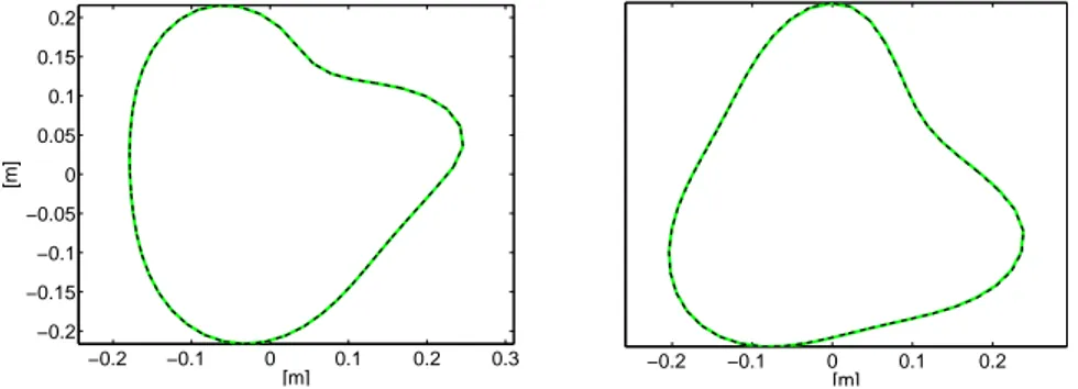
aδun o = 0 aδun k = −Unα nk(1 − n2)(1 − k2) π [EIk2(1 − k2) − ω2 onσoR4(1 + k2)] n sin[(n − k)Θ + ϕn] − sin(ϕn) 2(n − k) −sin[(n + k)Θ + ϕn] − sin(ϕn) 2(n + k) o bδun k = −Unα nk(1 − n2)(1 − k2) π [EIk2(1 − k2) − ω2 onσoR4(1 + k2)] n cos[(n − k)Θ + ϕn] − cos(ϕn) 2(n − k) +cos[(n + k)Θ + ϕn] − cos(ϕn) 2(n + k) o (23) In figure 3 and 4 the modal perturbations δuncorresponding, respectively, to n = 2 and n = 3 have been
plotted considering as baseline the undeformed ring. The increment α of bending stiffness due to the reinforce is equal to 20% of the ring bending stiffness EI, and the reinforce spans the angle [0, 75o). Each
eigenmode δunhas been rescaled such as the maximum absolute value among its radial and tangential
nodal displacement components is equal to R/4. As a comparison, the corresponding curves evaluated by using the finite element method have been superimposed with dotted line; the agreement is quite satisfying.
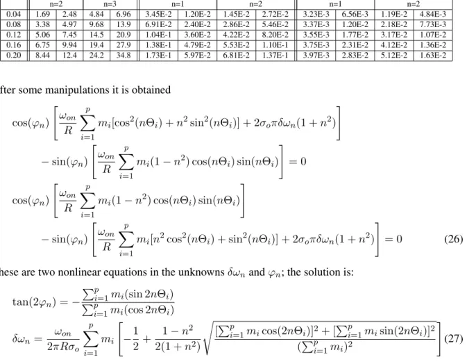
In table 2 the frequency splits δωn are reported, evaluated according to the proposed method, as
a function of the ratio γ = α/EI, while keeping fixed the angle spanned by the reinforce as chosen previously. Moreover the relative difference δωn% between the frequency splits and the relative l2norm
δun% between the modal shape perturbations δun, evaluated using the proposed model and the finite
element model, are also reported. The results in the table show that the proposed method is very accurate both in evaluating the frequency splits δωnand the perturbations δun of the modal shapes, even in the
−0.2 −0.1 0 0.1 0.2 0.3 −0.2 −0.15 −0.1 −0.05 0 0.05 0.1 0.15 0.2 [m] [m] −0.2 −0.1 0 0.1 0.2 [m]
Figura 3: Perturbation δunrelevant to n = 2 due to a reinforce; continuous line: theory, dotted line: fem
−0.2 −0.1 0 0.1 0.2 −0.2 −0.15 −0.1 −0.05 0 0.05 0.1 0.15 0.2 [m] [m] −0.2 −0.1 0 0.1 0.2 0.3 [m]
Figura 4: Perturbation δunrelevant to n = 3 due to a reinforce; continuous line: theory, dotted line: fem
4.2 Case 2
It is here considered a imperfect ring, as shown at the right hand side of fig. 2, whose imperfection is due to p lumped masses miadded at angles θ = Θi. As a consequence the bending stiffness EI is constant
on all the ring whereas the linear density σ is given by
σ(θ) = σo+ p
X
i=1
αiδ(θ − Θi) (24)
where σois a constant, αi = mi/R and δ is the Dirac distribution. The two existence conditions (11) for
the solution of the perturbed dynamical problem are specialized to the present case as follows:
ωon p
X
i=1
αi[cos(nΘi+ ϕn) cos(nΘi) + n2sin(nΘi+ ϕn) sin(nΘi)] + 2σoπδωn(1 + n2) cos(ϕn) = 0
ωon
p
X
i=1
αi[cos(nΘi+ ϕn) sin(nΘi) − n2sin(nΘi+ ϕn) cos(nΘi)] +
Tabella 2: Comparison results between theoretical and fem model; imperfection due to a reinforce applied to the ring
γ δωn[rad/s] δωn% δun%
n=2 n=3 n=1 n=2 n=1 n=2
0.04 1.69 2.48 4.84 6.96 3.45E-2 1.20E-2 1.45E-2 2.72E-2 3.23E-3 6.56E-3 1.19E-2 4.84E-3
0.08 3.38 4.97 9.68 13.9 6.91E-2 2.40E-2 2.86E-2 5.46E-2 3.37E-3 1.20E-2 2.18E-2 7.73E-3
0.12 5.06 7.45 14.5 20.9 1.04E-1 3.60E-2 4.22E-2 8.20E-2 3.55E-3 1.77E-2 3.17E-2 1.07E-2
0.16 6.75 9.94 19.4 27.9 1.38E-1 4.79E-2 5.53E-2 1.10E-1 3.75E-3 2.31E-2 4.12E-2 1.36E-2
0.20 8.44 12.4 24.2 34.8 1.73E-1 5.97E-2 6.81E-2 1.37E-1 3.97E-3 2.83E-2 5.12E-2 1.63E-2
After some manipulations it is obtained
cos(ϕn) " ωon R p X i=1 mi[cos2(nΘi) + n2sin2(nΘi)] + 2σoπδωn(1 + n2) # − sin(ϕn) " ωon R p X i=1 mi(1 − n2) cos(nΘi) sin(nΘi) # = 0 cos(ϕn) " ωon R p X i=1 mi(1 − n2) cos(nΘi) sin(nΘi) # − sin(ϕn) " ωon R p X i=1 mi[n2cos2(nΘi) + sin2(nΘi)] + 2σoπδωn(1 + n2) # = 0 (26)
These are two nonlinear equations in the unknowns δωnand ϕn; the solution is:
tan(2ϕn) = − Pp i=1mi(sin 2nΘi) Pp i=1mi(cos 2nΘi) δωn= 2πRσωon o p X i=1 mi " −1 2 + 1 − n2 2(1 + n2) s [Ppi=1micos(2nΘi)]2+ [ Pp i=1misin(2nΘi)]2 (Ppi=1mi)2 # (27)
The first of (27) correspond to two values of ϕndiffering from each other by an angle of π/2; these two
values, once substituted in the second of (27) yield two different values of the frequency split δωn. In
order to evaluate the coefficients relevant to the series expansion of δun, the equations (15) are taken into account and specialized to the present case; the coefficients of δunread as:
aδun o = − Un πσoR p X i=1 micos(nΘi+ ϕn) aδun k = Un ω2 on π£EIR3k2(1 − k2)2− Rωon2 σo(1 + k2) ¤ × p X i=1
mi[cos(nΘi+ ϕn) cos(kΘi) + nk sin(nΘi+ ϕn) sin(kΘi)]
bδun k = Un ω2 on π£EIR3k2(1 − k2)2− Rω2onσo(1 + k2) ¤ × p X i=1
In the special case of just one lumped mass added (p=1), (27) reduces to: ϕn1= −nΘ, ϕn2= −nΘ +π 2 δωn1 = −2πσM ωon oR(1 + n2), δωn2= − n2M ω on 2πσoR(1 + n2) (29)
In figures 5 and 6 the modal perturbations δuncorresponding, respectively, to n = 2 and n = 3 have
been plotted, due to a lumped mass M equal to 5% of the ring mass applied at θ = 0.
−0.2 −0.1 0 0.1 0.2 −0.15 −0.1 −0.05 0 0.05 0.1 0.15 [m] [m] −0.2 −0.1 0 0.1 0.2 −0.2 −0.15 −0.1 −0.05 0 0.05 0.1 0.15 [m] [m]
Figura 5: Perturbation δunrelevant to n = 2 due to an added mass; continuous line: theory, dotted line: fem
−0.2 −0.1 0 0.1 0.2 −0.15 −0.1 −0.05 0 0.05 0.1 0.15 [m] [m] −0.2 −0.1 0 0.1 0.2 [m]
Figura 6: Perturbation δunrelevant to n = 3 due to an added mass; continuous line: theory, dotted line: fem
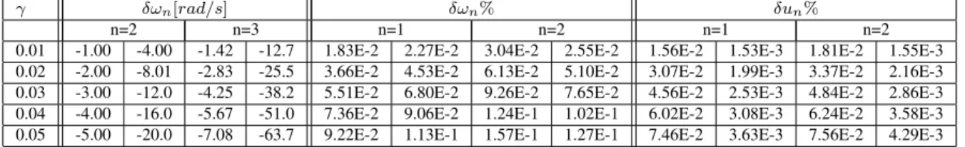
In table 3 quantities analogous to those of table 2 are reported, referred to the case of added lumped mass. The parameter γ = M/(2πRσ) is the ratio between the added lumped mass and the mass of the ring, which is kept fixed at θ = 0.
Tabella 3: Comparison results between theoretical and fem model; imperfection due to a lumped mass attached to the ring
γ δωn[rad/s] δωn% δun%
n=2 n=3 n=1 n=2 n=1 n=2
0.01 -1.00 -4.00 -1.42 -12.7 1.83E-2 2.27E-2 3.04E-2 2.55E-2 1.56E-2 1.53E-3 1.81E-2 1.55E-3
0.02 -2.00 -8.01 -2.83 -25.5 3.66E-2 4.53E-2 6.13E-2 5.10E-2 3.07E-2 1.99E-3 3.37E-2 2.16E-3
0.03 -3.00 -12.0 -4.25 -38.2 5.51E-2 6.80E-2 9.26E-2 7.65E-2 4.56E-2 2.53E-3 4.84E-2 2.86E-3
0.04 -4.00 -16.0 -5.67 -51.0 7.36E-2 9.06E-2 1.24E-1 1.02E-1 6.02E-2 3.08E-3 6.24E-2 3.58E-3
0.05 -5.00 -20.0 -7.08 -63.7 9.22E-2 1.13E-1 1.57E-1 1.27E-1 7.46E-2 3.63E-3 7.56E-2 4.29E-3
Also in the present case the agreement between results provided by the proposed approach and by the finite element model is quite good, both in terms of frequency split prediction and in terms of modal perturbation evaluation.
5. CONCLUSIONS
The dynamics of a imperfect ring has been studied in this paper. The imperfections were modeled as small perturbations of the linear density and the in-plane bending stiffness of the ring, depending on the angular variable. A first-order perturbation expansion was employed in order to derive a differential equation governing the eigenmode perturbation. Closed-form expressions for the perturbed eigenmodes and eigenfrequencies have been found out considering a Fourier series expansion of the linear density and bending stiffness of the ring. Finally some case-study problems have been considered in order to compare the analytical results with analogous results obtained using a finite element model.
AKNOWLEDGEMENTS
This research was developed within the framework of Lagrange Laboratory, an European research group between CNRS, CNR, University of Rome “Tor Vergata”, University of Montpellier II, ENPC and LCPC.
REFERENCES
[1] A.K. Rourke, S. McWilliam, C.H.J. Fox, “Frequency trimming of a vibrating ring-based multi-axis rate sensor,” Journal of Sound and Vibration, Vol. 280, 2005, pp. 495–530.
[2] B.J. Gallacher, J. Hedley, J.S. Burdess, A.J. Harris, A. Rickard, D.O. King, “Electrostatic correction of structural imperfections present in a microring gyroscope,” Journal of Microelectromechanical Systems, Vol. 14 (2), 2005, pp. 221–234.
[3] J. Tang, K.W. Wang, “Vibration delocalization of nearly periodic structures using coupled piezoelectric networks,” ASME Journal of Vibration and Acoustics, Vol. 125, 2003, pp. 95–108. [4] X. Fang, J. Tang, E. Jordan, K.D. Murphy, “Crack induced vibration localization in simplified
bladed-disk structures,” Journal of Sound and Vibration, Vol. 291, 2006, 395–418.
[5] C.H.J. Fox, “A simple theory for the analysis and correction of frequency splitting in slightly imperfect rings,” Journal of Sound and Vibration, Vol. 142 (2), 1990, pp. 227–243.
[6] R.S. Wwang, C.H.J. Fox, S. McWilliam, “The in-plane vibration of thin rings with in-plane profile variations part I: general background and theoretical formulation,” Journal of Sound and Vibration, Vol. 220 (3), 1999, pp. 497–516.
[7] P.A.A. Laura, C.P. Filipich, R.E. Rossi, J.A. Reyes, “Vibrations of rings of variable cross section,” Applied Acoustics, Vol. 25, 1988, pp. 225–234.
[8] S. McWilliam, J. Ong, C.H.J. Fox, “On the statistics of natural frequency splitting for rings with random mass imperfections,” Journal of Sound and Vibration, Vol. 279, 2005, pp. 453–470. [9] R. Eley, C.H.J. Fox, S. McWilliam, “Anisotropy effects on the vibrations of circular rings made