Mixed Mode Fracture Behaviour of Piezoelectric Materials

(1)

Alma Mater Studiorum – Università di Bologna

Facoltà di Ingegneria

***

D.I.S.T.A.R.T.

SEDE DI SCIENZA DELLE COSTRUZIONI

Dottorato di Ricerca in Meccanica delle Strutture

XXII ciclo

Coordinatore

Chiar.mo Prof. Ing. Erasmo Viola

Mixed Mode Fracture Behaviour

of Piezoelectric Materials

Tesi di Dottorato di

Claudia Boldrini

Relatore

Prof. Ing. Erasmo Viola

S.S.D. ICAR 08

(2)

(3)

iii

PRESENTAZIONE DELLA TESI DI DOTTORATO

di CLAUDIA BOLDRINI

Lo studio presentato in questa Tesi di Dottorato si inserisce nell’ambito della trattazione analitica della Meccanica della Frattura.

Il tema principale del lavoro svolto è la risposta elettro-elasto-statica alla frattura di un mezzo piezoelettrico fessurato, in regime di carico tensionale ed elettrico biassiale all’infinito.

Per la trattazione analitica è stato adattato al caso piezoelettrico un formalismo, analogo a quello di Stroh, che era precedentemente stato utilizzato per il più semplice caso dei materiali ortotropi [Piva, 1987; Piva e Viola, 1988]. Questo metodo, attraverso l’applicazione del teorema spettrale dell’algebra sulla matrice fondamentale, permette di esprimere le equazioni governanti il problema elastico mediante dei potenziali complessi. In seguito, con l’imposizione delle condizioni al contorno (meccaniche ed elettriche) sui bordi del crack, ci si riconduce a un problema di Hilbert, la cui soluzione è nota.

Un primo aspetto, ampiamente discusso in letteratura, che è stato affrontato in questa ricerca è stato la definizione delle opportune condizioni al contorno elettriche da imporre ai bordi della discontinuità (fessura). In questa tesi sono state analizzate le soluzioni per tre diversi modelli di fessura (crack permeabile, impermeabile e semi-permeabile al campo elettrico), ed i risultati ottenuti sono stati confrontati per cercare di quantificare quale sia l’importanza della corretta scelta del modello da applicare, verificando che in molti casi questo è un aspetto tutt’altro che trascurabile.

Un altro aspetto analizzato con attenzione è stato l’influenza dell’applicazione di un carico biassiale, ed in particolare l’effetto del carico collineare alla direzione del

(4)

iv

crack. Mentre il caso di un carico biassiale è stato ampiamente trattato in letteratura per quanto riguarda il caso dei materiali isotropi [ad esempio Carpinteri et al., 1979; Eftis et al., 1990] od ortotropi [ad esempio Lim et al., 2001; Carloni et al., 2003], esso non è stato quasi mai considerato per la frattura nei materiali piezoelettrici. Il carico collineare compare solo nell’espressione dei termini non singolari della soluzione del problema elettroelastico. La tendenza prevalente è di considerare solo la parte asintotica della soluzione nell’analisi del campo tensionale nell’intorno della fessura, dal momento che questa è inversamente proporzionale alla distanza r dal tip del crack e quindi predominante nelle sue immediate vicinanze. L’eliminazione dei termini non singolari dalla soluzione implica però il trascurare la possibilità che anche una forza parallela alla direzione del crack possa esercitare un’influenza sul campo elettroelastico riscontrato nei pressi della discontinuità. Nella nostra analisi i termini non singolari sono stati ritenuti, ed attraverso una simulazione numerica del comportamento di diverse ceramiche piezoelettriche i risultati così ottenuti sono stati confrontati con quelli asintotici. Per valutare la possibile propagazione della fessura all’interno del materiale sono stati utilizzati due diversi criteri: il criterio della massima tensione circonferenziale [Erdogan e Sih, 1963], ed il criterio della minima densità di energia di deformazione [Sih, 1973]. Un interessante risultato ottenuto è la dimostrazione che la presenza di un carico collineare può avere conseguenze macroscopiche per quanto riguarda lo studio dell’angolo di diramazione della fessura. Infatti, secondo entrambi i criteri suddetti, l’applicazione di un carico sufficientemente elevato parallelo al crack provoca una brusca diversione dall’orizzontale della direzione di estensione della lesione, pur in condizioni di carico simmetrico (cioè in assenza di forze tangenziali applicate). Dallo studio analitico si evince quindi che l’effetto della biassialità del carico non è assolutamente trascurabile nello studio dei problemi di frattura; sarebbe importante avvalorare i risultati analitici con prove sperimentali.

Nella seconda parte di questa tesi sono riportati i risultati di una ricerca sperimentale a cui ho collaborato durante un periodo di soggiorno come Visiting

(5)

v

Researcher presso il Department of Mechanical Engineering, The City College of New York, nell’A.A. 2008/09.

L’obiettivo del progetto di ricerca (tuttora in corso) è la validazione di una tecnica self-sensing per la rilevazione di danni da delaminazione in elementi strutturali laminati compositi. La tecnica utilizza la resistenza elettrica trasversale di un laminato composito come principale parametro per l’individuazione della presenza e propagazione di un crack interlaminare. Il principio alla base è che la presenza o la propagazione di un crack di delaminazione ingeneri una diminuzione della conduttività elettrica trasversale nella zona in prossimità del danno, con conseguente aumento della resistenza. La tecnica tradizionale prevede sensori a due terminali, che sono utilizzati sia per applicare la corrente elettrica, sia per misurare la differenza di potenziale e conseguentemente la resistenza. Il limite di questo metodo è che la resistenza così misurata non è solo quella del materiale che si vuole testare, ma anche quella del filo attraverso cui viene fatta passare la corrente e dell’elettrodo stesso. In particolare nel caso di una non perfetta connessione dell’elettrodo al materiale, l’errore così introdotto può non essere trascurabile. Per ovviare a questo problema è stata proposta una seconda tecnica a quattro elettrodi, dove i primi due sono utilizzati per il passaggio della corrente ed i secondi due, posti nelle immediate vicinanze, per la misurazione della resistenza, permettendo di eliminare dalla misura l’impedenza dei cavi.

La ricerca ha lo scopo principale di capire i limiti di applicazione e la potenzialità del metodo e di esplorarne le possibilità di utilizzo industriale. Una tecnica di self-sensing potrebbe ridurre o eliminare l’utilizzo di sensori quali MEMS o piezoelettrici, correntemente utilizzati nel monitoraggio automatico dell’integrità strutturale. I dati ricavati dimostrano quasi sempre che all’avanzare della delaminazione lungo il provino corrisponde un aumento del valore registrato della resistenza, indicando che la tecnica self-sensing può essere una promettente metodologia di diagnostica strutturale.

(6)

vi

Tutti i test sono stati effettuati presso il Laboratorio di Meccanica dei Materiali del City College of New York. Alcuni dei risultati dei test sono stati presentati al convegno International Conference on Integrity, Reliability and Failure, tenutosi a Porto, 20-24 Luglio 2009.

(7)

vii

Outline

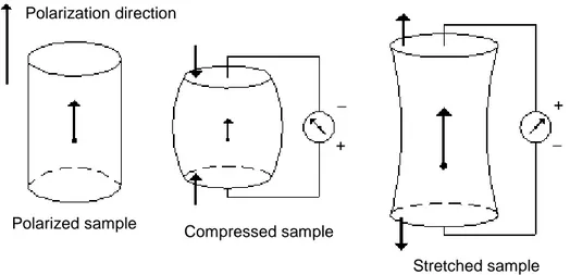
Piezoelectrics present an interactive electromechanical behaviour that, especially in recent years, has generated much interest since it renders these materials adapt for use in a variety of electronic and industrial applications like sensors, actuators, transducers, smart structures. Both mechanical and electric loads are generally applied on these devices and can cause high concentrations of stress, particularly in proximity of defects or inhomogeneities, such as flaws, cavities or included particles. A thorough understanding of their fracture behaviour is crucial in order to improve their performances and avoid unexpected failures. Therefore, a considerable number of research works have addressed this topic in the last decades.

Most of the theoretical studies on this subject find their analytical background in the complex variable formulation of plane anisotropic elasticity. This theoretical approach bases its main origins in the pioneering works of Muskelishvili and Lekhnitskii who obtained the solution of the elastic problem in terms of independent analytic functions of complex variables.

In the present work, the expressions of stresses and elastic and electric displacements are obtained as functions of complex potentials through an analytical formulation which is the application to the piezoelectric static case of an approach introduced for orthotropic materials to solve elastodynamics problems. This method can be considered an alternative to other formalisms currently used, like the Stroh’s formalism. The equilibrium equations are reduced to a first order system involving a six-dimensional vector field. After that, a similarity transformation is induced to reach three independent Cauchy-Riemann systems, so justifying the introduction of the complex variable notation. Closed form expressions of near tip stress and displacement fields are therefore obtained. In the theoretical study of cracked piezoelectric bodies, the issue of assigning consistent electric boundary conditions on the crack faces is of central importance and has been addressed by many researchers. Three different boundary conditions are commonly accepted in literature: the permeable, the impermeable and the semipermeable (“exact”) crack model. This thesis takes into considerations all the

(14)

4

three models, comparing the results obtained and analysing the effects of the boundary condition choice on the solution.

The influence of load biaxiality and of the application of a remote electric field has been studied, pointing out that both can affect to a various extent the stress fields and the angle of initial crack extension, especially when non-singular terms are retained in the expressions of the electro-elastic solution.

Furthermore, two different fracture criteria are applied to the piezoelectric case, and their outcomes are compared and discussed.

The work is organized as follows:

Chapter 1 briefly introduces the fundamental concepts of Fracture Mechanics. Chapter 2 describes plane elasticity formalisms for an anisotropic continuum (Eshelby-Read-Shockley and Stroh) and introduces for the simplified orthotropic case the alternative formalism we want to propose.

Chapter 3 outlines the Linear Theory of Piezoelectricity, its basic relations and electro-elastic equations.

Chapter 4 introduces the proposed method for obtaining the expressions of stresses and elastic and electric displacements, given as functions of complex potentials. The solution is obtained in close form and non-singular terms are retained as well.

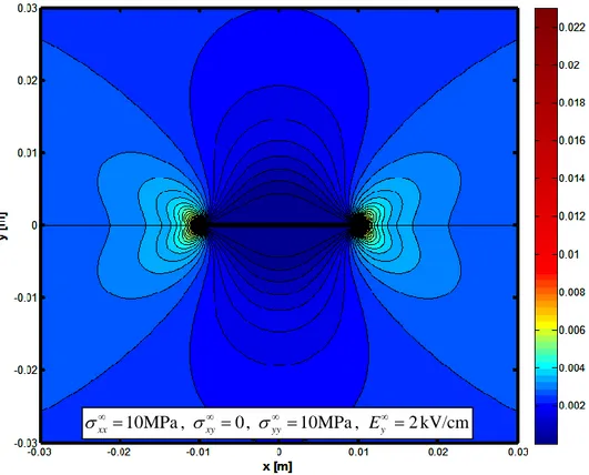
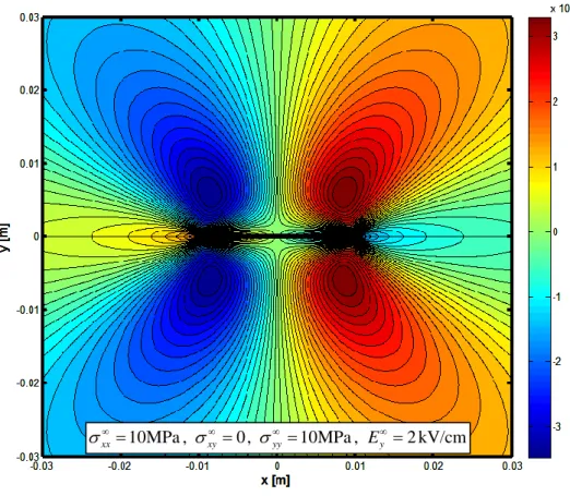
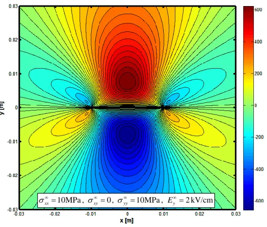
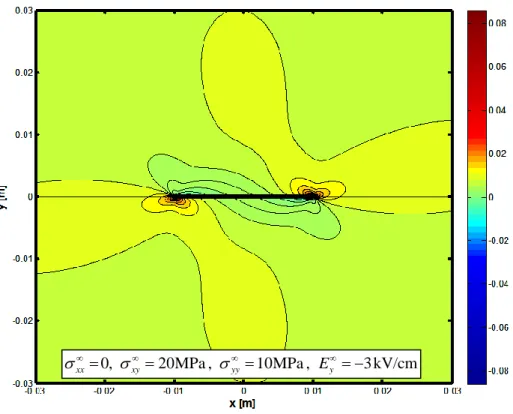
Chapter 5 presents several numerical applications aimed at estimating the effect of load biaxiality, electric field, considered permittivity of the crack. Through the application of fracture criteria the influence of the above listed conditions on the response of the system and in particular on the direction of crack branching is thoroughly discussed.

Finally, Appendix A lists a few mathematical definitions and concepts useful for understanding some algebraic steps of the analysis, and Appendix B reports the explicit form of the fundamental matrix of the electro-elastic problem.

(15)

5

NOMENCLATURE

a Griffith crack semilength B Biot’s generalized free energy

ijks

c elastic constants of material

v

C specific heat per unit mass

i

D ,D_i components of electric displacement and of electric displacement applied at infinity

0 y

D electric displacement at the crack surfaces

sij

e piezoelectric constants of material

s

E ,Es

 _{components of electric field and of electric field applied at infinity}

bi f body force ( ) ( ) , k k j j

g h real and imaginary parts of element f_j( )k of eigenvector f( )k

g _{Gibbs function} G Energy Release Rate

I

K ,K_II,K_D stress intensity factors (Mode I, Mode II and electric)

,

k k

p q real and imaginary parts of eigenvalues _k

b

q electric charge density

/

r a ratio of distance from crack tip on crack semilength s entropy density

1 xx/ yy

s    ratio of collinear on perpendicular remote loads

2 xy/ yy

s    ratio of tangential on perpendicular remote loads

S Sih’s Energy Density a

T absolute temperature

,

u v elastic displacement components

m

 pyroelectric coefficients

ks

 strain tensor components

is

 dielectric constants of material

c

 permittivity of the medium inside the crack

k

 eigenvalues

 electric potential

(16)

6 ij  ,ij



components of stress tensor and of mechanical loading applied at infinity   hoop stress

 

k zk  complex potentials



k1, 2,3



,

  a b Stroh’s eigenvectors (1) ( 2) (3) , ,

f f f eigenvectors corresponding to eigenvalues   ₁, ₂, ₃

1, 2

t t generalized stress vectors 1, 2

 

t t remote loading vectors (1) ( 2)

,

Γ Γ generalized strain vectors

( )z

Λ analytic vector null at infinity U generalized displacement vector U Airy’s stress function

(17)

7

CHAPTER 1 BASIC CONCEPTS OF FRACTURE MECHANICS

1.1 Introduction

It is common knowledge learned from experience that cracks can be very detrimental to strength, even when small. Cracks running rapidly through hard structural materials (metal, rocks, concrete) are also within common experience. The cracking or complete fracture is often so rapid that it is difficult to detect with eyes the sudden extension from some small initial defect, notch hole or other irregularities. Such irregularities are extremely important because they modify the state of stress in their immediate neighbourhood, usually introducing a local intensification.

Until the material in question does not fail, the calculation of the fields of stress and strain around the crack can be carried out by solving a boundary value problem in some kind of idealized body. The calculation of stress and strain in the vicinity of a crack in the process of extending requires consideration of a sequence of ordinary boundary value problems, as well as of some additional conditions in order to know when the boundary undergoes a change.

The two basic problems in Fracture Mechanics are therefore the evaluation of stress and strain fields around the crack tip and the knowledge of the conditions under which a crack can extend into a medium [1].

1.2 Modes of fracture and stress intensity factors

Some basic definitions of Fracture Mechanics are now introduced, referring for simplicity to an isotropic material, and along with Williams’s method [2,3], that sought the solution of the fracture problem expressing it in terms of Airy’s

(18)

bi-8

harmonic stress function. For brevity we will report the results only, referring to the work in bibliography for further details.

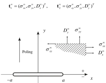
Consider first a crack of length 2a , embedded in an isotropic elastic continuum plate subjected at infinity to biaxial load (Fig. 1.1). A plane state of strain is considered.

2a

Fig. 1.1 – Geometry of the crack problem

It can be useful to consider also a polar coordinate system centred in the right tip of the crack. We will also suppose the crack faces to be free from applied stresses, which means applying the boundary conditions:



r,



_r



r,



0

 

     (1.1)

The general loading condition illustrated in Figure 1.1 can be decomposed into the sum of a symmetric (Figure 1.2) and an anti-symmetric (Figure 1.3) load, which yield symmetry and anti-symmetry conditions on the stresses as well.

1.2.1. Symmetric plane problem (Mode I)

Stress components must comply to the symmetry conditions:

 





 





 





r r r r r , r , r , r , r , r ,                        (1.2) xy  yy T  _ xx kT  _ y x r 

(19)

9

The general solution of the differential system is a linear combination of the particular solutions:

 

1

 

1 n n n r, r f     



U (1.3)

where U

 

r, is Airy’s stress function. This yields the following expressions for

the stress components:

 

1 2 1 1 2 1 1 2 1 1 2 1 2 2 2 n r n n n n n n n r n n n r f f n n r f n r f           _   _   _   _     _ _  _ _          _ _  _ _      _    _ _  



(1.4) 2a

Fig. 1.2 – Symmetric problem

Equations (1.4) show that the first terms of the series (for n1) present an inverse square root singularity of the radial distance from the crack tip. In the vicinity of the crack tip, for r1, the asymptotic representations of stress fields,

in Cartesian coordinates, are therefore [4,5,6]:

3 cos 1 sin sin

2 2 2

2

3 cos 1 sin sin

2 2 2

2

3 sin cos cos

2 2 2 2 I xx I yy I xy K r K r K r                 _       _      (1.5) yy T  _ xx kT  _ y x r 

(20)

10

where the relations between Cartesian and polar coordinates:





2 2

cos sin sin2

sin cos sin2

sin2 cos sin 2 xx r r yy r r r xy r                                      (1.6)

have been used, and where K_I is a constant. From equation (1.5)-2, for  0 and switching to the variable 

 

x  x a, one obtains the definition of KI:

 



  

0 lim 2 0 lim 2 0 I yy yy r x a K  r r, r x a  ,      (1.7)

which is called stress intensity factor for the first (opening) mode.

It is to be noted that the applied collinear load _xx_{does not appear in the}

asymptotic representations of the stress fields (1.5).

1.2.2. Anti-symmetric plane problem (Mode II)

For the anti-symmetric problem, symmetry conditions for the stress components are:

 





 





 





r r r r r , r , r , r , r , r ,                         (1.8) 2a

Fig. 1.3 – Anti-symmetric problem

Through the boundary conditions (1.8) and (1.1), superposing the particular solutions and considering only the first terms of the series, that present inverse square root singularities of r , one gets for the stress components, in Cartesian coordinates:

xy

 _

y

(21)

11

3 sin 2 cos cos

2 2 2

2

3 cos sin cos

2 2 2

2

3 cos 1 sin sin

2 2 2 2 II xx II yy II xy K r K r K r                   _  _    _      (1.9)

where K_II is a constant. From equation (1.9)-3, for  0 and switching to the variable 

 

x  x a, one obtains the definition of K_II:

 



  

0 lim 2 0 lim 2 0 II xy xy r x a K  r r, r x a  ,      (1.10)

which is called stress intensity factor for the second (sliding) mode.

1.2.3. Anti-plane problem (Mode III)

There is a third basic fracture mechanism, characterised by the presence of only two stress components:

 

0

xx yy zz xy zx zx x, y , zy zy x, y

         (1.11)

For this mechanism, caused by out-of-plane shear, Williams obtained: sin 2 2 2 III rz III z K r K r         (1.12) where:



  

lim 2 0 III _x _a z K r x a  _ ,    (1.13)

is called stress intensity factor for the third (tearing) mode.

The superposition of the three modes describes the general case of fracture. In particular for the plane case, of major concern in this study, we have [7]:

 

I II 2 2 ij I II ij ij K K f f r r        (1.14)

The whole (asymptotic) stress field at the crack tip is known when the stress intensity factors are evaluated [7]. This asymptotic representation gives a sufficiently accurate description of the problem in the vicinity of the crack, although some authors [8-14] have noted that retaining the second terms of the series can be extremely important to study the effect of biaxial load.

The stress components are proportional to the external load, they vary with the square root of the crack size and tend to infinity at the crack tip.

(22)

12

The elastic solution does not prohibit that the stresses become infinite at the crack tip. In the reality this does not occur: plastic deformation takes place. An evaluation of the size of the crack tip plastic zone can be obtained using the yield criterion [15,16].

It should be noted that in this work attention will be focused on the elastic behaviour of a cracked plate, thus, outside the plastic zone.

1.3 Fracture criteria for crack initiation

A fracture criterion is a constitutive equation stating the critical condition of a crack on the verge of branching. Among the local criteria generally used to predict the critical stress conditions and the angle of incipient fracture, the Maximum Normal Stress Criterion [17,18] and the Strain Energy Density Theory [15,16,19,20] will be discussed.

Note that the abovementioned criteria refer to the study of crack initiation. This means that the attention is focused on the incipient crack propagation.

In what follows the fracture criteria are applied to isotropic materials.

1.3.1 Maximum Circumferential Tensile Stress Theory

For isotropic materials, the circumferential stress _, defined as:

2 2

11sin 22cos 12sin 2 

       (1.15)

can be studied to analyse the crack extension angle, for plane problems.

According to this criterion, crack extension occurs in the direction of the maximum circumferential stress __{evaluated at a small distance} r₀ from the crack tip, sufficient to be outside the plastic zone [16]. Designating the polar angle that defines the direction of extension as ₀, the following conditions must be satisfied for the circumferential stress to be maximized:

0 0     _  (1.16)

 

_ _{ }₀ 0    _  (1.17)

 

₀ 2 2    0    _  (1.18)

The crack extension begins as soon as the following situation is reached:

0 0 2 IC K r        (1.19)

(23)

13

where K_IC is the critical value of the stress intensity factor K_I which is defined at the onset of crack initiation. This is a material parameter and is also referred to as the fracture toughness of the material.

1.3.2 Strain Energy Density Theory

Referring to the problems of fracture mechanics, the strain energy per unit of volume can be expressed as [15,16,19,20]:

d d

W S

V  r (1.20)

S is the strain energy density factor and it is related to the stress intensity

factors as follows:

2 2

11 I 2 12 I II 22 II

Sa K  a K K a K (1.21) where the coefficients aij are defined by:







11 1 3 4 cos 1 cos 16 a      _    _ (1.22)









12 1 2sin cos 1 2 16 a      _   _ (1.23)





 





22 1

4 1 1 cos 1 cos 3cos 1 16

a    



 _      _ (1.24)

and  is the second Lamé constant of elasticity.

Note that the strain energy density criterion allows to consider all the three modes of fracture together [15], and so it can be used to predict crack initiation in spatial problems, despite of the first criterion.

The fundamental hypotheses of crack extension according to the Strain Energy Density Theory can be summarized as follows. The crack will spread in the direction of the minimum strain energy density, and the critical value of S (say,

cr

S ) governs the onset of the crack propagation. Summarizing, the crack begins to propagate in the ₀ direction when the following conditions are satisfied:

 

S _{ }₀ 0      (1.25)

 

₀ 2 2 S   0    _  (1.26) 0 cr S _{ }_ S (1.27)

The critical value of S is a material parameter and for the isotropic case it is related to K_IC.

(24)

14

References

[1] Liebowitz H., (edited by) Fracture: An advanced treatise (Vol.II), Academic Press, New York, 1968.

[2] Williams M.L., On the stress distribution at the base of a stationary crack, J. Appl. Mech. 24, Trans. ASME, vol. 79 (1957), 109-114.

[3] Irwin G. R., Fracture, in: «Handbuch der Physik», vol. 6, Springer, Berlin (1958), 551-590.

[4] Broek D., Elementary Engineering Fracture Mechanics, Noordhoff International Publishing, Leyden, The Netherlands, 1974.

[5] Viola E., In tema di sviluppi asintotici all’apice di una fessura rettilinea, Nota Tecnica 128, Università di Bologna, Facoltà di Ingegneria, DISTART, A.A. 1991-92

[6] Viola E., Deduzione non tradizionale del metodo di Westergaard per

problemi di meccanica della frattura, Nota Tecnica 129, Università di

Bologna, Facoltà di Ingegneria, DISTART, A.A. 1991-92

[7] Sih G.C., Handbook of stress intensity factors, Institute of Fracture and Solid Mechanics, Bethlehem, Pennsylvania, 1973.

[8] Eftis J., Subramonian N., Liebowitz H., Biaxial load effect on the crack

border elastic strain energy and strain energy rate, Engng. Fract. Mech.

(1977); 9: 753-764.

[9] Eftis J., Subramonian N., Liebowitz H., Crack Border Stress and

Displacement Equations Revisited, Engng. Fract. Mech. (1977); 9: 189-210.

[10] Eftis J., Subramonian N., The inclined crack under Biaxial Load, Engng. Fract. Mech. (1978); 10: 43-67.

[11] Liebowitz H., Lee J.D., Eftis J., Biaxial Load Effects in Fracture Mechanics, Engng. Fract. Mech. (1978); 10: 315-335.

[12] Liebowitz H., Lee J.D., Subramonian N., Theoretical and experimental

biaxial studies, Proc. Int. Symp. Fract. Mech., George Washington

(25)

15

[13] Viola E., Influenza delle tensioni non singolari sulla direzione di diramazione

di un crack dominante in regime biassiale, Giornale del Genio Civile, Fasc.

I, II, III, 1979.

[14] Viola E., Non-singular stress effects on two interacting equal collinear

cracks, Engng. Fract. Mech. (1977); 18: 801-814.

[15] Sih G.C., A special theory of crack propagation: methods of analysis and

solutions of crack problems, Mechanics of Fracture I, Noordhoff, Leyden,

The Netherlands, 1973.

[16] Sih G.C., Mechanics of Fracture initiation and propagation, Kluwer Academic Publisher, 1991.

[17] Erdogan F., Sih G.C., On the crack extension in plates under plane loading

and transverse shear, J. Basic Engng. (1963); 85: 519-527.

[18] Di Tommaso A., Nobile L., Viola E., Diramazione di un crack dominante in

un solido a regime de formativo biassiale, Atti del III Congresso Nazionale

dell’Associazione Italiana di Meccanica Teorica e Applicata, Cagliari, 1976. [19] Sih G.C., Cracks in composite materials, Mechanics of Fracture VI,

Noordhoff, Leyden, The Netherlands, 1981.

[20] Sih G.C., Strain density factor applied to mixed mode crack problems, Int. J. Fract. (1974); 10:305-321.

(26)

(27)

17

CHAPTER 2 PLANE ELASTICITY FORMALISMS FOR ANISOTROPIC

MATERIALS

2.1 Introduction

In this chapter, the displacement components u and the generalized stress _i

vectors t and ₁ t for anisotropic materials in plane deformation conditions are ₂ defined through Stroh’s formalism [1-3]. The Stroh’s formalism can be traced to the work of Eshelby-Read-Shockley (1953) [4], which therefore will be presented first. Furthermore, in the simplified case of an orthotropic material, an alternative formalism is introduced, and the relations between this last formulation and Stroh’s one are outlined.

2.2 Eshelby-Read-Shockley’s formalism

In a Cartesian coordinate system



x x x let ₁, ₂, ₃



u and _i _ij



i j, 1, 2,3



be the displacement and stress components in an anisotropic elastic material, respectively.

Hooke’s law and the equilibrium condition can be expressed in index form as:

, k ij ijks k s ijks s u c u c x      (2.1) and:

(28)

18 2 , , 0 k ij j ijks k sj ijks s j u c u c x x        (2.2)

where addition on repeated index is implicit, and where the stiffness tensor components c_ijks satisfy the symmetry conditions:

, ,

ijks jiks ijks jisk ijks ksij

c c c c c c (2.3)

For two-dimensional deformations where u _i



i1, 2,3



only depend on



x x , a ₁, ₂



general solution for the homogeneous second-order differential equation system (2.2) is a function of one composite variable which is a linear combination of variables x and ₁ x . ₂

Let us assume:



1, 2



 

, 1 2, 1, 2,3

i i i

u u x x a f z z x px i (2.4)

where f is an arbitrary function of z, p and a are constants to be determined, _i

and the coefficient for x in the linear combination was chosen to be unity. In ₁

matrix form:

 

f z



u a (2.5)

Differentiation of in x and ₁ x yields: ₂

 

1 2 ' , ' k k k k u u a f z pa f z x x  _  _   (2.6) or:



1 2



'

 

k s s k s u p a f z x    _ _  (2.7)

where si is the Kronecker Delta. From (2.7):









 

2 1 2 1 2 '' k j j s s k j s u p p a f z x x      _ _ _   (2.8)

and so equilibrium is satisfied when:



1 2





1 2



0

ijks j j s s k

c  p  p a

    

  (2.9)

where sum is implicit on repeated indexes. Expliciting (2.9):

















3 2 1 2 1 2 1 1 3 2 1 1 2 2 1 2 1 0 : 0 ijks j j s s k j s ijk j j ijk j j k j c p p a c p c p p a                    _ _ _  _  





(29)

19





2

1 1 2 1 1 2 2 2

: _c_{i k}  c_{i k} c_{i k} p c _{i k} p _a_k 0 (2.10) and passing to the matrix form:



T



2

p p

     

Q R R T a 0 (2.11)

where the elements of the three 3x3 matrices are defined as follows:

1 1, 1 2, 2 2

ik i k ik i k ik i k

Q c R c T c (2.12)

One can verify that matrices Q and T are symmetric, as the equalities ci k1 1ck i1 1

and ci k2 2ck i2 2 hold, and positive-definite, in order for the energy of elastic

deformation to be positive. For the homogeneous system (2.11) to admit solutions different from the trivial one, it must be:





2

det_Q RRT pTp _0 (2.13) which is a sixth-grade equation in the eigenvalue p and yields three pairs of complex conjugate roots. Being p_, a_



 1, 2,...., 6



the eigenvalues and the correspondent eigenvectors solutions of the 6-grade equation, one can assume:

Imp_ 0 for1, 2,3 (2.14)

3 3 1, 2,3

p__  p_ a__ a  (2.15)

where the overbar denotes the complex conjugate.

The components of the stress vector can be obtained through (2.1); one gets:

 

  



 

1 1 1 ' 1 2 ' ' 1, 2,3 i ci k a fk z ci k pa fk z Qik pRik a fk z i       (2.16) and:

 

  



 

2 2 1 ' 2 2 ' ' 1, 2,3 i ci ka fk z ci k pa fk z Rki pTik a fk z i       (2.17)

One can define the generalized stress vectors as:



 

  

1 11 21 31 ' T p f z       t Q R a (2.18)









 

2 12 22 32 ' T T p f z       t R T a (2.19)

The components of the displacement vector can be obtained through (2.5) by superposing six solutions. With the assumption that the six eigenvalues, and consequently the six eigenvectors, are distinct, and from (2.14) one gets:

 

3 3

 

1, 2,3

f z f z

          

u a u a (2.20)

(30)

20

 

6 3 3 1 1 f z  f z            







_  _ u u a a (2.21)

Likewise, the general solutions for the stresses can be written as:





 





 

3 1 3 1 ' ' p_ _{ }f z_ p_ f _ z_     



_    _ t Q R a Q R a (2.22)





 





 

3 2 3 1 ' ' T T p_ _{ }f z_ p_ f _ z_     



_    _ t R T a R T a (2.23) 2.3 Stroh’s Formalism

From equation (2.11) one obtains:



T







p p p

   

R T a Q R a (2.24)

One can define a vector b such as:



T



1





p p

p

    

b R T a Q R a (2.25)

whose components are:





1





i ki ik k ik ik k

b R pT a Q pR a

p

     (2.26)

where the sum on index k 1, 2,3 is implicit. The components of the stress

vectors can now be expressed as:

 

1 ' 2 ' 1, 2,3

i pb fi z i b fi z i

      (2.27)

Introducing the stress functions:

 

i b f zi

  (2.28)

expressions (2.27) can be written as:









1 ,2 1 2 2 ,1 1 2 2 1 i i b f xi px i i b f xi px x x       _  _     _  _   (2.29)

It is sufficient therefore to consider the stress functions i, because stresses can be

obtained by differentiation. Since 2112, we have:

1,1 2,2 0

   (2.30)

and so, from (2.28):

1 2 0

(31)

21

Vectors b are correlated to vectors  a via the relation (2.25), so for them as

well the position b__₃ b with  1, 2,3 holds. The general solution of the plane

problem can be obtained through superposition of the six particular solutions associated to the six eigenvalues p_, in the form:

 

3 3 1 f z f z          



_  _ u a a (2.32)

 

3 3 1 f z f z          



_  _ Φ b b (2.33)

Relations (2.32) and (2.33) express the Stroh’s Formalism, and vectors a and 



b are called Stroh’s eigenvectors. The stress vectors can be obtained by differentiation of (2.33). The only stress component missing is 33, which can be

determined in terms of other stress components using the condition for ₃₃ 0. In many plane problems the arbitrary functions f_ have the same shape. We may therefore assume:

 

, 3

   

1, 2,3

f_ z_  f z_ q_ f__ z_  f z_ q_  (2.34)

where q_ are arbitrary complex constants. The second equation is necessary for obtaining real form solutions for u and Φ, when superposing f_. Expression (2.32) becomes:

 





 

3 1 11 21 31 12 1 1 22 2 2 32 3 3 13 23 33 11 21 31 1 1 12 22 32 2 2 13 23 33 3 3 0 0 0 0 0 0 f z q f z q a a a a f z q a f z q a f z q a a a a a a f z q a a a f z q a a a f z q            _  _             _ _ _ _ _ _                           _ __ __{ }        



u a a conjugate terms co



njugate terms



(2.35) and in matrix form:

 

2 Re f zk 

 _ _ _ _

u Adiag q (2.36)

where A is the 3x3 matrix whose columns are eigenvectors a . Analogously _ (2.33) becomes:

(32)

22

 

2 Re f z_k 

 _ _ _ _

Φ Bdiag q (2.37)

where B is the 3x3 matrix whose columns are eigenvectors b_.

For a given problem it is necessary to determine the unknown function f z

 

_k

and the complex vector q.

The eigenvalues p_ and the eigenvectors a and b_ _ depend on the elastic stiffnesses c_ijks only. Therefore, p_, a and b_ _ can be regarded as material constants even though they are complex-valued.

2.4 Ortogonality and closure relations

What distinguishes the Stroh’s formalism from others is that the vectors a and _ b_ for different  are related. The complex matrices A and B possess some

peculiar properties [5,6].

From equations (2.24) and (2.25) one gets: p

Qa Ra b (2.38)

T

p

R a b  Ta (2.39)

which in matrix notation become:

T p         _            Q 0 a R I a R I b T 0 b (2.40)

where I is the 3x3 identity matrix. On the basis that T is positive definite and

therefore 1

T exists, it can be demonstrated that:

1 1          _           R I I 0 0 T T 0 0 I I RT (2.41)

Pre-multiplying both sides of (2.40) by the first matrix on the left of (2.41) gets:

1 1 1 T p 1                _ _    _              Q 0 a R 1 a 0 T 0 T R 1 b T 0 b 1 RT 1 RT 1 1 1 1 : T p               _ _ _   _         0 T Q a 0 T R a b 1 RT R a b 1 RT T a 1 1 ( ) : ( ) T T p          _ _ _ _        a T R a b b Q a RT R a b

(33)

23 1 1 1 1 : T T p             _ _           a a T R T b b RT R Q RT (2.42) Defining: 1 T 1 1 T 1 , 2 , 3         N T R N T N RT R Q (2.43) and: 1 2 T 3 1        N N N N N (2.44)

the following standard eigenrelation is obtained:

p ,    _{  }   a N ξ ξ ξ b (2.45)

The 6x6 matrix N is called the fundamental elasticity matrix. Since N is not symmetric, ξ is a right eigenvector. Denoting by η the left eigenvector, the following eigenrelation holds:

T p



N η η (2.46)

Introducing the 6x6 constant matrix:

T 1 ,    _ _     0 I I I I I I 0 (2.47)

it can be shown that IN is symmetric, or:

T T ( )   IN IN N I (2.48) From (2.45) we have: p  INξ Iξ (2.49) and by (2.48): ( ) ( ) T p  N Iξ Iξ (2.50)

The left eigenvector has therefore the form:

   _{  }   b η Iξ a (2.51)

It is known that the right and left eigenvectors corresponding to different eigenvalues are orthogonal to each other, i.e. for p_  p_ the following relation holds:

(34)

24

0

  

η ξ (2.52)

The vector ξ, and hence the vector η, are unique up to an arbitrary multiplier. It is convenient to normalize them such that:

1 2 6 , , , ,...,       η ξ (2.53) or: 1 2 1 2 6 6 T ( , , ..., )                      _{ } _         η ξ (2.54)

where  is the Kronecker delta. This condition yields:

1 1 2 2 3 3 1 1 2 2 3 3 1

T T T

T  T  T    

η ξ η ξ η ξ η ξ η ξ η ξ (2.55)

and all other products equal to zero. Introducing two 6x6 matrices such as:

1 2 3 1 2 3 ( , , , , , )  U ξ ξ ξ ξ ξ ξ (2.56) 1 2 3 1 2 3 ˆ ( , , , , , )   V η η η η η η 1U (2.57)

one can express the orthonormality conditions (2.54) as:

T _ V U I (2.58) Now, since; 1 1 1 1 2 2 2 2 3 3 3 3 1 4 1 4 2 5 2 5 3 6 3 6 b a b a b a , b a b a b a                                                                               _ _{ } _       _ _{ } _                             _ _{ } _     _ _{ } _ b a ξ η a b (2.59)

matrix U gets the shape:

1 2 3 3 1 2 1 2 3 3 1 2 11 31 11 31 13 33 13 33 13 33 13 33 , , , , , a a a a a a a a b b b b             ___{   } _{ } _{     }__                    _{ } _    _{ } _  _{ } _       a a a a a a U b b b b b b A A B B (2.60)

(35)

25 1 2 3 3 1 2 1 2 3 3 1 2 , , , , ,               _           _                  b b b b b b B B V a a a a a a A A (2.61) and thus: T T T T T    _ _   B A V B A (2.62) The orthogonality relations (2.58) assume the aspect:

T T T T T  _ _{ } _ _ __ _{ } _       B A A A I 0 V U 0 I B B B A (2.63) or: T T T T T T T T         B A A B I B A A B B A A B 0 B A A B (2.64) From (2.63) one can deduce that matrices U and V are the inverses of each other, and hence their product commute:

T T T T T T        _ __ _ _     _  B A I 0 A A V U UV 0 I B B _B _A (2.65)

from which we obtain the relations:

T T T T T T T T         A B A B I B A B A A A A A 0 B B B B (2.66) that are the closure relations. Equations (2.66) imply that the real part of T

AB is / 2

I , while AA and T BB are purely imaginary. The eigenrelation (2.45) can be T written as: 1 2 3 1 2 3 1 2 3 1 2 3 ( , , , , , )( , , , , , ) N ξ ξ ξ ξ ξ ξ ξ ξ ξ ξ ξ ξ P (2.67) where: 1 2 3 1 2 3 (p p p p p, , , , ,p )  P diag (2.68) We get:  N U U P (2.69)

that through (2.65) can be diagonalized as:

T 

N U P V (2.70)

The derivations presented so far assume that the eigenvalues p_ are distinct, or that anyway six independent eigenvectors ξ_ exist.

(36)

26

2.5 The case of orthotropic materials

In the case of an orthotropic material, and for a plane problem, the matrix of elastic constants is simplified as follows:

11 12 12 22 44 55 66 0 0 0 0 0 0 0 0 0 0 0 0 0 0 0 0 0 0 c c c c c c c                  C (2.71)

Consequently, matrices Q ,R and T defined in the Stroh’s formalism become:

11 12 66 66 66 22 55 44 0 0 0 0 0 0 0 0 , 0 0 , 0 0 0 0 0 0 0 0 0 c c c c c c c c             _ _ _ _ _ _             Q R T (2.72) and:













2 11 66 12 66 2 2 12 66 66 22 2 55 44 0 0 0 0 T c p c c c p p p c c p c p c c p c          _   _  _    Q R R T (2.73)

The characteristic equation is:



₂

 

₂



₂







2 ₂ 55 44 66 22 11 66 12 66 0 c  p c _ c  p c c p c  c c p _ (2.74) Posing 2 2 1 p   (2.75) yields:





2 44 55 2 4 2 2 11 66 66 11 22 12 66 22 66 0 0 c c c c c c c c c c c         _ _        _ _  (2.76)

Dividing the second equation by c c and with the positions: 11 66

66 22 12 66 12 66 1 1 1 1 1 2 1 11 66 11 66 , , 2 , 2 , 2 4 , c c c c c c a a c c c c                (2.77) equation (2.76)-2 becomes: 4 2 1 2 2a a 0      (2.78)

(37)

27

Equation (2.78) has no real solution. It is necessary to distinguish two cases: the four eigenvalues are imaginary or complex conjugate.

2.5.1. Imaginary Eigenvalues

This case happens when:

2

1 2 0, 1 0

a a  a  (2.79)

The four imaginary eigenvalues are:

1 2 1 i ,k1 2 i ,k2 3 , 4         (2.80) with



2



1 2



2



1 2 1 1 1 2 , 2 1 1 2 k  a  a a k  a  a a (2.81) positive constants.

2.5.2. Complex conjugate eigenvalues

This case happens when:

2 1 2 0 a a  (2.82) One gets: 2 2 1 a1 i a2 a1      (2.83) 2 2 1 a1 i a2 a1     (2.84)

and the two pairs of conjugate roots are:

2 2 1,1 1 2 1 1,2 1 2 1 2 2 2,1 1,2 1 2 1 2,2 1,1 1 2 1 +i , i , i , i a a a a a a a a a a a a                        (2.85) If we impose 2 i 1+i 2 1 2e a a a a     and 2 -i 1 i 2 1 2e a a a a      we can obtain: i 2 4 4 1 2 2 1 2 -i 2 4 4 2 2 2 1 2 3 1 4 2 e cos sin 2 2 e cos sin 2 2 , a a i i a a i i                     _  _          _  _       (2.86) where:

(38)

28 1 2 1 2 2 1 2 1 4 4 1 2 cos , 2 2sin 2 2 2 2 a a a a a  a    _  _   _  _     (2.87)

Furthermore, the first equation of (2.76) yields:

44 3 3 55 , c ik k c    (2.88)

From the system (2.73), six eigenvalues (either imaginary or complex conjugate) have been found; these can now be ordered considering first those with positive imaginary part: Case 1) 1 2 3 4 1 5 2 6 3 1 2 3 , , , , , i i i p p p p p p p p p k k k       (2.89) Case 2) i -i 2 2 1 2 3 4 1 5 2 6 3 4 4 3 2 2 1 1 e , e , i , , , p p p p p p p p p k a a          (2.90)

We now consider for the sake of simplicity the first case only, and proceed with the calculations of the correspondent eigenvectors. Through equations (2.74) for

1, 2 j :









2 11 66 12 66 1 2 12 66 66 22 2 2 55 44 3 0 0 0 0 0 j j j j j j j j c p c c c p a c c p c p c a c p c a          _ _  _        _ _ _   (2.91)

From the third equation, being



2



55 j 44 0

c  p c  for j1, 2, it is obviously yielded

3 0

j

a  . The first and the second equation can be outlined in the shape:









2 1 2 2 1 1 1 2 1 2 0 2 1 0 j j j j j j j j p a p a p a p a           (2.92) so we can set:



2



1 1 1 2 , 1, 2 0 j j j j j p p j      _              a (2.93)

(39)

29

and then choose the arbitrary factor j  1. With this position the first equation

becomes the characteristic one and the second is always satisfied. For j3 the

system is:









2 11 3 66 12 66 3 31 2 12 66 3 66 3 22 32 2 55 3 44 33 0 0 0 0 0 c p c c c p a c c p c p c a c p c a       _ _   _        _ _ _   (2.94)

whose solution is a₃₁a₃₂0, a₃₃ ₃ with ₃ arbitrarily chosen constant.

Stroh’s matrix A is then:







 



2 2 1 1 1 2 1 2 3 1 1 1 2 3 1 1 0 2 2 0 0 0 p p p p                       A a a a (2.95)

From the definition of vectors bj one gets:





6612 2266 12 44 3 0 0 0 0 j j T j j j j c p c a p c c p a c p a           _ __ _         b R T a (2.96)

thus Stroh’s matrix B can be written as:



1 2 3



12 1166



1 1122 1 1212



1266



212 2122 22222



44 3 33 0 0 0 0 c p a a c p a a c a c p a c a c p a c p a        _   _     B b b b (2.97)

or, by setting the arbitrary factor ₃

44 3 1 c p   :



1 2 3



12 1166



1 1122 1 1212



1266



212 2122 22222



0 0 0 0 1 c p a a c p a a c a c p a c a c p a        _   _     B b b b (2.98)

From Stroh’s matrices A and B, through relations (2.36) and (2.37) it is possible

to calculate the displacement vector u and the generalized potential vector Φ, and from this through relation (2.29) one gets the stress components.

Mixed Mode Fracture Behaviour of Piezoelectric Materials

Alma Mater Studiorum – Università di Bologna

Facoltà di Ingegneria

***

Dottorato di Ricerca in Meccanica delle Strutture

XXII ciclo