Modelling flow and heat transfer in helically coiled pipes - Part 4: Direct numerical simulation (DNS) of turbulent flow and heat transfer in the case of zero pitch

Sigla di Identificazione Distrlb. Pago

~

Ricerca Sistema Elettrico

NNFISS - LP2 - 021

L

Titolo

Modelling flow and heat transfer in helically coiled pipes

Part 4: Direct numerical simulation (DNS) of turbulent flow and heat transfer in the case of zero pitch

Ente emittente CIRTEN

PAGINA DI GUARDIA

Descrittori

Tipologia del documento: Rapporto tecnicol Technical Report

1

Collocazione contrattuale: Accordo di programma ENEA-MSE: tema di ricerca "Nuovo nucleare da fissione"

Argomenti trattati: Reattori ad acqua leggeralLight Water Reactors

Sommario

di

46

That report has been issued in the frame of the second research programme of ENEA-MSE agreement and it is one of the deliverables of the task G "Theoretical and experimental studies on IRIS criticaI components (SG, EHRS)" of the work-programme 2 "Evolutionary INTD reactors" of the research theme on "Nuovo Nucleare da Fissione".

The document reports the results of Direct Numerical Simulation of fully turbulent flow and heat transfer in toroidal pipes characterized by different ratio between pipe radius and torus radius (O, 0.1 and 0.3). The caIcuIations have been perfonned with ANSYS-CFX code using hexahedral volumes.

Note Copia n. In carico a:

2

NOME FIRMA 1 NOME FIRMA

O

1-fl!r1èID

NOME F. !!ianchi

EMISSIONE

~/

CIRTEN

C

ONSORZIO

I

NTERUNIVERSITARIO PER LA

R

ICERCA

T

ECNOLOGICA

N

UCLEARE

UNIVERSITA’ DI PALERMO

DIPARTIMENTO DI INGEGNERIA NUCLEARE

Modelling flow and heat transfer in

helically coiled pipes

Part 4: Direct Numerical Simulation (DNS) of turbulent flow and heat

transfer in the case of zero pitch

Modellazione numerica del campo di moto

e dello scambio termico in condotti elicoidali

Parte 4: Simulazione Numerica Diretta (DNS) del moto turbolento con

scambio termico nel caso di passo nullo

F. Castiglia, P. Chiovaro, M. Ciofalo, M. Di Liberto, P.A. Di Maio,

I. Di Piazza, M. Giardina, F. Mascari, G. Morana, G. Vella

CIRTEN-UNIPA RL-1207/2010

Palermo, Dicembre 2009

Lavoro svolto in esecuzione delle linee progettuali LP2 punto G dell’AdP ENEA MSE del 21/06/07, Tema 5.2.5.8 – “Nuovo Nucleare da Fissione”

CONTENTS

ABSTRACT 3

NOMENCLATURE 4

Greek symbols 4

Subscripts / superscripts 5

1. INTRODUCTION: FLOW AND HEAT TRANSFER IN CURVED PIPES AND COILS 7

1.1. Problem definition 7 1.2. Early studies 7 1.3. Transition to turbulence 8 1.4. Friction 9 1.5. Heat transfer 9 1.6. Recent studies 10

2. MODELS AND METHODS 11

2.1. Numerical methods 11

2.2. Computational mesh 11

3. PRELIMINARY RESULTS AND VALIDATION 13

3.1. Comparison with literature results for straight pipes 13 3.2. Comparison with literature results for curved pipes 14

4. RESULTS AND DISCUSSION 14

4.1. Range of parameters explored 14

4.2. Core inviscid balances 15

4.3. Near-wall behaviour 18

4.4. Turbulence and statistics 19

5. CONCLUSIONS 22

REFERENCES 24

TABLE 1 26

ABSTRACT

Direct Numerical Simulations of turbulent flow and heat transfer in toroidal pipes for Re14 000 are described in this report. Three different curvatureswere examined, i.e.=0 (straight pipe), 0.1 and 0.3. The Prandtl number was 0.86, representative of water at 500 K and 60 bar. The finite volume code ANSYS-CFX was used, with computational grids of 11.5106_{hexahedral volumes for the smaller}

curvature torus (=0.1) and 3.4106 _{volumes for=0.3 and for the straight pipe. In the latter case, the}

computational domain was 10 times the pipe diameter in length. Simulations were protracted for 30 LETOT’s starting from the condition of zero velocity.

Time–averaged results for curved pipes showed Dean circulation and a strong velocity and temperature stratification in the torus radial direction; most of the core flow features were compatible with simple inviscid momentum balances. Secondary flow markedly influenced the structure of turbulence; velocity and temperature fluctuations in curved pipes were mainly confined to some specific areas of the near-wall layer. In the outer region, counter-gradient heat transport by turbulent fluxes was observed. For the same Reynolds number, turbulence levels were lower than in a straight pipe. The Reynolds momentum-heat transfer analogy was found to hold globally, but not locally.

NOMENCLATURE

a pipe radius [m]

c torus radius [m]

cp specific heat [J kg1K1] De Dean number,

Re 

f local Darcy friction coefficient,

4 /

 

w



u

2av

/ 2



0

f

equilibrium Darcy friction coefficient

N number of grid points

Nu local Nusselt number,

q

_w

 

2

a

 

(

T

_b

T

_w

)



Pr Prandtl number

p pressure [Pa]

ps opposite of streamwise pressure gradient [Pa m-1]

P dimensionless pressure,

_/

 

2

av

p



u

q heat flux [W m-2_]

r radial coordinate in the cross section [m]

rp radial coordinate from torus axis [m]

R dimensionless radius, r/a

Re bulk Reynolds number, uav2a/ Re friction Reynolds number,

u a

0

/



s thickness of secondary flow boundary layer [m]

S dimensionless boundary layer thickness, s/a

T temperature [K]

T local wall temperature scale,

q

_w

/

 



c u

_{p } [K]

u velocity [m s-1_]

u local friction velocity,

 

_w

/

[m s-1] 0

u

_ equilibrium friction velocity, 0

_/

w

 

[m s-1_]

U dimensionless velocity, u/uav

y+ _{distance from the wall in wall units,}

_yu

0

/





Greek symbols

 dimensionless curvature, a/c

 dissipation [m2_s-3_]

 thermal conductivity [W m-1_K-1_]

 kinematic viscosity [m2_s-1_]

 density [kg m-3_]

K Kolmogorov length scale [m]

 azimuthal angle in the pipe’s cross section [°]

 dimensionless temperature, (T-Tw)/(Tb-Tw)



shear stress [Pa]

0

w



equilibrium wall shear stress, psa/2 [Pa]

 similarity quantity,

8 Nu/ RePr f





Subscripts b bulk

cr critical

Dean related to Dean circulation

eff effective

LAM laminar

RAD radial

rp radial direction from torus axis

s,r, streamwise (axial), radial and azimuthal directions

sp straight pipe sec secondary tot total w wall  azimuthal Superscripts 0 equilibrium

+ expressed in wall units

Averages

 azimuthal average



time average

1. INTRODUCTION: FLOW AND HEAT TRANSFER IN CURVED

PIPES AND COILS

1.1. Problem definition

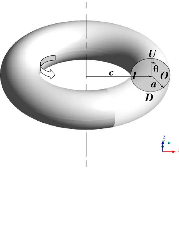
Fig. 1 shows a schematic representation of a closed toroidal pipe; the torus radius, i.e. the radius of curvature, will be indicated by c, while the cross-section radius by a. The inner, outer, up and down sides will be indicated by I, O, U, D, respectively; the cross-section azimuthal angle will be measured in the clockwise direction looking from upstream, with (I)=-/2, (O)=/2. The bulk Reynolds number Re will be defined on the basis of the pipe diameter 2a and the cross-section averaged (bulk) velocity uav as

Re



u

_av

2 /

a



,being the kinematic viscosity of the fluid. The friction-velocity Reynolds number will be defined as

_Re

_{u a}

0

_/









on the basis of the equilibrium

friction velocity 0 0

_/

w

u

_



 

, being. 0

_{( / 2)}

w

a

p

s

 

the equilibrium wall shear stress and ps the streamwise driving pressure gradient. Finally, the curvature will be defined as = a/c.

An important engineering application of curved pipes are helical coils, which are used for heat exchangers and steam generators in power plants because they are compact and easily accommodate thermal expansion. Several theoretical fundamental studies have appeared in the last decades on this geometry [1-3]; these works show that coil torsion, which characterizes a helical pipe with respect to a toroidal one, has only a higher order effect on flow features, and, if sufficiently low, does not significantly affect global quantities such as friction and heat transfer coefficients.

1.2. Early studies

The earliest studies of flow in curved pipes are due to Boussinesq [4] and Thomson [5] in the 19th

century. Later, Grindley and Gibson [6] noticed the effect of curvature on the fluid flow during experiments on the viscosity of air. Williams et al. [7] observed that the location of the maximum axial velocity is shifted towards the outer wall of a curved pipe. Eustice [8] showed the existence of a secondary flow by injecting ink into water. Early studies have been recently reviewed, for example, by Di Piazza and Ciofalo [9]. A thorough literature review of flow in curved pipes has been presented by

A more quantitative approach was proposed by Dean [11], who wrote the Navier-Stokes equations in a toroidal reference frame, and, under the hypothesis of small curvatures and laminar stationary flow, derived a solution for the stream function of the secondary motion and for the main axial velocity, both expanded in power series; the first term of the series corresponds to the Hagen-Poiseuille flow. From his analysis a new governing parameter emerged, now called the Dean number

De Re 



, which couples together inertial, centrifugal and viscous effects. Although Dean originally based his number on the maximum velocity in a straight pipe under the same pressure gradient, most of the authors later used the average axial velocity in the curved pipe uav, and we will follow this strain; the Dean equations can be properly reformulated using this latter scale [10].

1.3. Transition to turbulence

As regards transition to turbulence, Cioncolini and Santini [12], for sufficiently high values of the curvature (> 0.0416), observed a smooth transition from laminar to turbulent flow; the equilibrium Darcy friction coefficient

f

0 (four times the Fanning coefficient) decreased monotonically with Re and transition to turbulence was indicated only by a change in slope of the

f

0_{-Re curve, occurring at}

a Reynolds number which the authors approximated by the correlation:

0.47

Re

_cr



30000





(1)

in the range 0.0416 0.143. For lower curvatures (< 0.0416), Cioncolini and Santini observed that in the proximity of transition the

_f

0_{-Re curves exhibited a local minimum followed by an}

inflection point and by a local maximum; also in this range of they proposed transition correlations, more complex than Eq. (1) and based on identifying transition with the local minimum of

f

0, i.e. with the first departure from the laminar behaviour. Similarly, Ito [13] gave an upper bound for the applicability of the laminar flow friction correlation, which can be identified with a transition criterion:



0.6



Re

cr



2000 1 13.2





(2)

Also Srinivasan et al [14] studied the transition to turbulence on the basis of friction coefficient measurements and arrived at a similar conclusion. The authors proposed their own correlation for the critical Reynolds number in curved pipes:





Re

cr



2100 1 12





(3)

Unlike Eq. (1), Eqs. (2) and (3) exhibit the correct asymptotic behaviour for= 0 and show that the effect of curvature is to delay transition to turbulence with respect to straight pipes. For typical values of the curvature, Eqs. (1) through (3) yield similar values of Recr; for example, they predict Recr = 10 069, 10 165 and 8631, respectively, for = 0.1, and Recr = 17 036, 14 820 and 15 902, respectively, for= 0.3. Note, however, that the latter case is outside the range of validity of Eqs. (1) and (2).

1.4. Friction

Experimental investigations of friction in curved pipes in a wide range of curvatures and Reynolds numbers are presented by Ito [13], who derived accurate correlations for the equilibrium friction coefficient

f

0 _{in the laminar and turbulent ranges:}

0 5.73 10

64

21.5 De

Re (1.56 log De)

f

 





(laminar flow) (4) 0

_{0.304 Re}

0.25

_0.029

f











(turbulent flow) (5)

valid for 5104_{0.2. Eqs. (4) and (5) have recently been confirmed by the extensive experimental}

work of Cioncolini and Santini [12] in a wide range of curvatures (2.7103 _{0.143) and Reynolds numbers (Re=10}3_-7104_{): the authors found a good agreement}

with Ito’s correlations both in the laminar and in the fully turbulent range.

Eq. (5) can be regarded as a correction to Blasius’ resistance formula for straight pipes,

0

_{0.316 Re}

0.25

f

_

_



(turbulent flow) (6)

1.5. Heat transfer

for the inner (tube) side will be used:



2



Nu

w b w

q

a

T

T









(7)

where qw is the local wall heat flux, is the fluid’s thermal conductivity, Tb is the bulk fluid temperature and Twis the wall temperature (which is uniform in the present simulations). In previous work [15], a systematic computational study of heat transfer in curved pipes in the fully turb ulent range was carried out. The study showed that an excellent reduction of the azimuthally averaged Nusselt number Nucan be obtained by applying the Pethukov momentum-heat transfer analogy [16] to curved pipes,

 





0 0 2/3

Pr Re

/8

Nu

1.07 12.7

/8 Pr

1

f

f









(8)

and using Ito’s formula, Eq. (5), for

f

0. It was shown that this approach is by far superior to any power–law dependence. For Pr1, Eq. (8) approximately reduces to the Reynolds analogy Nu=Re

0

f

_{/8. In the turbulent range, substituting Eq. (5) for}

_f

0 _{into Eq. (8) written for Pr1 yields}

Nu



Nu

sp

 

K

De

, where

Nu

sp is the average Nusselt number in a straight pipe at the same Reynolds number and K is a constant. Thus, the influence of curvature on heat transfer appears as an additive correction, proportional to the Dean number, to the straight pipe Nusselt number.

1.6. Recent studies

Numerical simulations of incompressible turbulent flow in helical and curved pipes are presented by Friedrich and co-workers [17-18]. The authors numerically solve the Navier-Stokes equations written in orthogonal helical coordinates [1] and compare toroidal and helical pipe results for Re5600 (Re230) and = 0.1. In a further paper [19] the same research group present the expression of the

Reynolds-stress balance equations in orthogonal helical coordinates. Although straight pipes would be in the turbulent regime at this Reynolds number, all the above transition criteria, Eqs. (1)-(3), predict that curved pipes with= 0.1 are in the laminar regime. Our previous simulations [9], conducted for the same curvature and Reynolds number, predicted a quasi-periodic flow characterized by the

presence of travelling waves, in agreement also with the experimental findings of Webster and Humphrey [20]. This latter regime is only apparently chaotic because it exhibits two incommensurate frequencies so that the temporal records of the various flow quantities do not exhibit any obvious periodicity. The classical statistical approach used for turbulent flow, based on the computation of the hierarchy of moments (averages and Reynolds stresses), is clearly inadequate in this case.

2. MODEL AND METHODS

2.1. Numerical methods

The geometry simulated was a torus with no slip conditions at the wall, as shown in Fig. 1. A constant source term ps in the axial momentum equation was adopted as the driving force which balances frictional pressure losses. This is equivalent to imposing the equilibrium wall shear stress

0

_{( / 2)}

w

a

p

s

 

and thus the equilibrium friction velocity 0 0

_/

w

u

_



 

.

As thermal boundary condition a uniform wall temperature Twwas imposed. In order to maintain a steady bulk-to-wall temperature difference, a local energy source term was applied to balance, at each time step, the integrated wall heat flux; due to the definition of the Nusselt number, Eq. (7), based on the bulk temperature Tb, this term must be proportional to the instantaneous and local axial velocity. Using this treatment, the fluid energy content, and thus the bulk temperature, remain constant during the simulation and statistically fully developed conditions are obtained. The Prandtl number was fixed to 0.86 in all cases, simulating water at 500 K and 60 bar.

For the numerical simulations presented in this paper, the ANSYS-CFX11™ code [21] was used, which is based on a finite-volume coupled algebraic multigrid solver. Hexahedral control volumes were used, with the central difference scheme for the advection terms and a second-order backward Euler time stepping scheme.

2.2. Computational mesh

The mesh is multi-block structured, and is characterized by the parameters NRADand Nas shown in

introduced at the wall, with a maximum/minimum cell size ratio of 4.7 in the radial direction. With these choices, the cross section was resolved by about 11 200 volumes, and the first near-wall grid point was well within the viscous sublayer (y+_{1) at Re14 000. In the axial direction the domain was} discretized by 1024 cells for=0.1 and by 300 cells for =0.3 and for the straight pipe; this led to an overall number of cells of 11.5106_{for the smaller curvature torus (=0.1) and of 3.410}6_{for=0.3 and}

for the straight pipe. For this latter case, the domain had an extension of 10 pipe diameters in the axial direction.

The Kolmogorov length scale

_{( / )}

3 1/ 4

K





 

can be expressed for the present configuration as



1/ 4



/ Re Re

K

a



 



. The present mesh provides a resolution of 2.6Kin the radial direction and 7-8Kin the axial direction. Taking account of near-wall grid refinement, these values are of the same order as those usually adopted in Direct Numerical Simulation of turbulence, see for example Kim et

al.[22].

However, for curved pipes the above estimate is excessively conservative. In fact, in this case part of the dissipation is not related to turbulence, but rather to the large scale secondary circulation: even in the turbulent regime, a significant fraction of the pumping power provided to the system is spent to maintain the Dean cells. The associated dissipationDean can be roughly estimated by extrapolating beyond its proper range of validity Ito’s resistance formula for

f

LAM0 , Eq. (4), while the total dissipationtotcan be assumed to be proportional to the overall friction factor

f

0 computed by DNS. This leads to an estimated turbulent dissipation



₁

0

_/

0



eff tot Dean tot

f

LAM

f

  

 







, and yields an actual Kolmogorov length scale



₁

0

_/

0



1/ 4

Keff K

f

LAM

f









 ; this latter quantity is 2-2.5for the

present Reynolds number and curvatures. Keeping this increase in into account, the actual

resolution for curved pipes is higher than for the straight duct, i.e. K in the radial direction and 3.5Kin the axial direction for both curvatures.

The time step was set to

_{0.8 / u}

 

0 2 



for all cases; this time discretization is sufficient to capture most of the turbulent variations, see Choi and Moin [23]. For the present axial grid, the above choice

guarantees a Courant number less than 1 in all cases.

Zero velocity and uniform temperature initial conditions were set for all the numerical simulations. Instabilities were spontaneously triggered by small numerical fluctuations due to truncation and round-off errors. The time necessary to achieve statistically steady conditions was about 15 LETOT’s

_{a u}

_/

0

 in all cases; 15 further LETOT’s were simulated in order to compute flow

statistics.

3. PRELIMINARY RESULTS AND VALIDATION

3.1. Comparison with literature results for straight pipes

The computational method was firstly validated for straight pipes, where a larger amount of computational and experimental data are available, and a higher turbulence level is expected with respect to curved pipes at the same Reynolds number. Toonder and Nieuwstadt [2 4] published experimental data on turbulent flow in straight pipes for Re=4900, 10 000, 17 800, and 24 000. The global friction coefficient computed by the authors is in agreement with the Blasius resistance formula, Eq. (6); for Re=14 400, the present DNS computation provides

f

0_{=0.0284, against values of}

0.0288 from Eq. (6) and 0.0289 from interpolation of the experimental data in [24]. The average Nusselt number Nuobtained in the present DNS is 44.3, very close to the value of 44.8 obtained by applying the Pethukov analogy, Eq. (8).

Fig. 3 shows a comparison of the time-averaged axial velocity profile (expressed in wall units) between the present DNS and the experimental data in [24] obtained for Re=17 800. The “law of the wall”, written in its high-Reynolds number form, is also reported. The DNS results slightly overestimate the experimental data and the law of the wall in the region y+_{20200, which is partly}

explained by the lower Reynolds number of the present DNS. For the same reason, the centreline corresponds to different values of y+ _{in the experiments and in the simulations. On the whole, the}

present results can be regarded as satisfactory, showing that the unresolved scales of turbulence play only a minor role.

3.2. Comparison with literature results for curved pipes

As regards curved pipes, no DNS or experimental data are available at Re14 000. Comparisons have been carried out with the numerical simulations presented in [17, 18] by Friedrich and co-workers for

=0.1 and Re5632 (Re230). This case and the complex physical phenomenology involved have

been fully discussed in reference [9]. Comparison is made here on the time-averaged fields. Friedrich and co-workers simulated a tract of the toroidal pipe 7.5 diameters in length, whereas in the present simulations the computational domain included the whole torus.

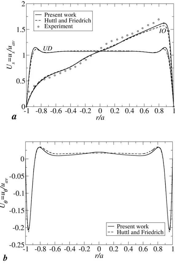
Fig. 4(a) shows the dimensionless axial velocity Us=us/uav as a function of the dimensionless radial coordinate r/a along the equatorial line IO, from the inner wall (r/a=-1) to the outer wall (r/a=1), and along the vertical midline DU, from the bottom wall (r/a=-1) to the top wall (r/a=1). In the latter case the problem’s symmetry (in the time averages) with respect to the torus equatorial midplane is evident. Symbols denote the experimental results obtained by Webster and Humphrey [20] for the same Reynolds number but a different curvature (=5.510-2_{). The agreement is very good}

with the numerical simulations and fair with the experimental data, despite the difference in curvature. It should be noticed that the radial gradient of the axial velocity in Fig. 4(a), once made dimensionless by uav/a, is 0.75, higher than the valuethat would be characteristic of a rigid body rotation. Thus a real flow in a curved channel shows a progressive sliding of the fluid layers from the I to the O sides, with the outer fluid overcoming the inner fluid.

Fig. 4(b) shows a comparison for the mean profile of the dimensionless azimuthal velocity

U=u/uav along the DU line, exhibiting characteristic near-wall peaks in the secondary (Dean) circulation boundary layer; the agreement with the computational results in [17, 18] is fully satisfactory also for this quantity.

4. RESULTS AND DISCUSSION

4.1. Range of parameters explored

Table 1 summarizes the three test cases presented in this paper. They cover three values of the curvature, i.e.=0 (straight pipe), 0.1 and 0.3, while the Reynolds number is about 14 000 in all cases. The three test cases are denoted by D1C for=0.1, D3C for =0.3 and D0C for the straight pipe. The

friction and bulk Reynolds numbers Re, Re are provided in Table 1; for comparison with other

studies, the Dean number De, as defined in section 1, is also reported. The equilibrium friction coefficient

f

0 _{can be computed simply as}

_f

0

_{32 Re / Re}





2





; the corresponding values

f

corr0 provided by the Blasius or Ito correlations, Eqs. (6) or (5), are included for comparison purposes. Finally, Nuis the Nusselt number computed by DNS while NuPis that predicted by the Petukhov analogy, Eq. (8), on the basis of the above values of

f

0_.

4.2. Core inviscid balances

Fig. 5 shows maps of the time-averaged axial velocity and temperature in the cross section for cases D1C and D3C. The axial velocity us is made dimensionless as Us= us/uav; the temperature T is made dimensionless as= (T-Tw)/(Tb-Tw), so that it is 0 at the wall while its bulk value is 1. A large-scale stratification along the horizontal direction, i.e. along the radius of the torus, is clearly visible for both curvatures. The shape of the iso-lines reflects also the presence of the secondary Dean circulation in the plane of the section; in fact, iso-lines are distorted by the secondary, inward-flowing, current in the upper and lower wall boundary layers and in the proximity of the Dean vortex centres in the inner side region.

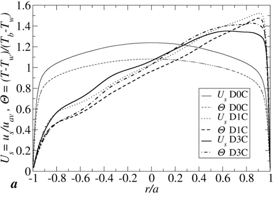
The horizontal stratification can be better evidenced by looking at the distributions of dimensionless velocity and temperature along the IO equatorial midline, reported in Fig. 6(a). For the straight pipe (case D0C) a clear symmetric behaviour can be observed, indicating a pure radial dependence, whereas, for curved pipes, all profiles in the core region collapse on a similar roughly linear behaviour characterized (in dimensionless form) by a slope of 0.75, regardless of the curvature value. As the curvature increases, only a moderate flattening of the profiles of Usand near the outer side can be observed (the reasons for this behaviour will be discussed in section 4.4).

The behaviour of the axial velocity usin the core region can be related to that of the radial velocity

urp along the radial coordinate rpwhich starts from the torus axis by an inviscid approximation of the axial momentum equation. By neglecting vertical velocities and observing that |us/c|«|us/rp|, this can be approximately written as:

s s rp p

u

p

u

r









(9) Observing that

_/

0



2

_{/ 2 / 2}



 

s av

p

  

p s

f



u

a

and using dimensionless variables Urp= urp/uav and Rp=rp/a, this can also be written as:

0

4

s p rp

U

f

R

U







(10)

This balance expresses the basic physical mechanism that shifts the axial velocity maximum towards the outer wall in a curved pipe.

Fig. 6(b) shows the profile of the dimensionless radial velocity Urpalong the I0 line. In the core region this quantity oscillates around 0.01, yielding, according to Eq. (10) and to the values of

_f

0 _in

Table 1,



U

s

/

 

R

p

1

. The relative maxima and minima of Urpin Fig. 6(b) correspond to the minima

and maxima in the slope of the velocity profiles in Fig. 6(a), as predicted by Eq. (10).

Similarly, the scale of the secondary motion can be estimated from a simple balance between centrifugal and inertial force in the cross section. By applying the work-kinetic energy theorem, the work per unit mass done by the mean centrifugal force 2

_/

av

u

c

equals the kinetic energy per unit mass of the secondary flow:

2 2 av sec sec av

u

u

a u

c





u





(11)

Here, Usec=usec/uav can be identified with the dimensionless velocity of the inward-flowing secondary flow boundary layers of dimensionless thickness S = s/a. Since the time-averaged secondary flow in the cross-section represents a closed circulation and a proper stream function can be defined for it, the dimensionless radial velocity Urpcan be obtained by a mass balance condition:

rp sec rp

u a u s





U



S



(12)

This allows one to re-write the momentum balance in Eq. (10) as:

0

_{/ 4}

s p

U

f

R

S









(13)

regardless of the Reynolds number and the curvature, the conclusion is that the dimensionless thickness S of the secondary boundary layer must be close to

 

_f

0

_{/ 4 /}

_

_{, which is confirmed by}

the numerical simulations.

By applying the same inviscid hypothesis to the radial momentum equation, the following relation between the dimensionless quantities

_/

 

2

av

P



p



u

, Rp and Usis obtained: 2 s p p

U

P

R

R







(14)

with the pressure gradient balancing the centrifugal force. Fig. 7(a) shows the profile of the ratio



2

_/



_/

_/



s p p

U

R

 

P R

along the IO line. This ratio is O(1) from r=-0.75 to r=0.75, i.e. in the core region, confirming the validity of the inviscid balance hypothesis. Therefore, at least for the present values of Re, both the viscous and the turbulent stresses are globally negligible in the core region, where inertia and pressure forces dominate; turbulence, if present, is confined to the near-wall layers.

As a consequence of the momentum-heat transfer analogy discussed above, for Pr1 dimensionless axial velocity and temperature exhibit in the core region the same roughly linear profile regardless of the curvature and of the Reynolds number, see Fig. 6(a). Therefore, the pressure gradient is tied both to the dimensionless velocity and to the thermal stratification, i.e.

2 2

/

_{p s}

/

_p

/

_p

P R

U

R



R

  



. Observing that, at the centre of the section, Us1, it follows that the order of magnitude of the radial pressure gradient

 

P R

/

p is , and therefore it is higher for the higher curvatures.

By integrating the inviscid balance in Eq. (14), it can be shown that, in the core region and for

«1, the dimensionless pressure has the analytic expression

2 3 2

3

P

b

R

bR

R









(15)

where b is the slope of the velocity profile in the core and R=Rp-1/. This is valid both for laminar stationary flow and for the time-averaged field in unsteady laminar flow [9] and turbulent flow. Results for this latter condition (cases D1C and D3C) are shown in Fig. 7(b), where the time-averaged

balance is more closely valid.

4.3. Near-wall behaviour Friction

Fig. 8 shows the time-averaged azimuthal profiles of the local wall shear stress w, normalized by the equilibrium value 0

w



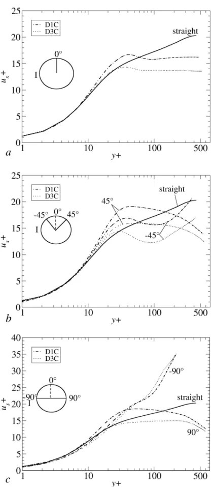
. The profiles are almost curvature-independent and exhibit a monotonic and approximately linear behaviour from=-60° to=60°, i.e. in the secondary, inward flowing, boundary layers. The wall shear stress decreases from the outer region (>0) to the inner region (<0), in correspondance with the thickening of the secondary flow boundary layers; a local minimum is present in the inner region at the location in which the secondary flow boundary layer detaches from the wall and enters the Dean vortex.

Figs. 9 (a) to (c) show near-wall profiles of the the axial velocity

u

_s _{as a function of y}+ _at different angles. Velocity and distance from the wall are normalized by the local friction velocity

/

w

u

_



 

and by the local wall length scale



/u

, respectively. With this normalization, velocity

profiles follow well the linear law in the viscous sublayer y+_{<10. All profiles show the absence of a} logarithmic region at any angle for both curvatures (straight pipe profiles are also reported for comparison purposes). For=0°, Fig. 9(a), the plateau in the core region, observed both for D1C and D3C, reflects the velocity stratification in theIO direction, see Fig. 5. For =-45°, Fig. 9(b), the most relevant feature is the influence of the Dean vortex which stretches the iso-lines and determines a local velocity minimum at about y+_{100. Fig. 9(c) shows the profiles for =90°, i.e. along the IO} direction. The very high value of the axial velocity (

u

s

35



_

) in the centre of the duct for=-90° is due to the low value of the wall shear stress in the region=-90°±20° of the inner wall side.

Heat Transfer

Fig. 10 shows the time-averaged azimuthal profiles of the local wall heat flux qw normalized by its overall average value qw. The profile for the lower curvature=0.1, case D1C, exhibits a monotonic and approximately linear behaviour from =-60° to=60°, like that of the wall shear stress in Fig. 8.

For the higher curvature=0.3, case D3C, the behaviour is not linear and tends to flatten in the outer region >0. The wall heat flux decreases from the outer region (>0) to the inner region (<0), in correspondence with the thickening of the secondary flow boundary layer. A local minimum is present in the inner region for D1C at the detachment point (-70°).

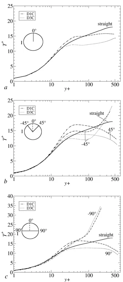
Figs. 11 (a) to (c) show the temperature profiles

T







T

w



T T



 as functions of y+at different

angular locations around the wall. Temperature is normalized with respect to the local wall temperature scale

T





q

w





c u

p 



. With this normalization, all profiles follow well the linear law in

the viscous/conductive sublayer y+_{<10. The behaviour at different angles is similar to that of the} axial velocity in Figs. 9 (a)-(c), and similar considerations hold.

Fig. 12 shows the local similarity quantity

 

8 Nu/ Re Pr f





as a function of the azimuthal angle ,

f



4 /

 

w



u

av2

/ 2



being the local Darcy friction coefficient. This quantity would be

identically 1 if the Reynolds analogy held on a local basis. For Pr1, this latter analogy was shown to apply well to the azimuthal averages for turbulent flows in straight and curved pipes [15] on the basis of RANS simulations. Fig. 12 shows that the analogy is confirmed for both curvatures also by the present DNS results as regards the azimuthally averaged quantities, since oscillates around 1. It approximately maintains its validity also locally for the lower curvature case D1C, with an error of less than 15%. On the contrary, for the higher curvature case D3C the error is more than 30% both on the inner and the outer regions of the wall, reflecting the different behaviour of the local wall shear stress, Fig. 8, and of the local heat flux, Fig. 10.

4.4. Turbulence and statistics Overview

Fig. 13 shows the instantaneous distribution of the quantityQ





2S 2



/ 2 in the generic cross section for cases D0C, D1C and D3C. Here, and S are the in-plane parts of the vorticity and strain rate tensors, respectively; the positive regions of Q define vortices, and (unlike the vorticity) Q goes to zero at the walls, making graphical representations clear.

The different spatial structure of turbulence is clearly evidenced by the comparison of the three pictures. D0C reveals the classical presence of vortices mainly located at a certain distance from the wall, but still present well within the core region which thus appears to be fully turbulent; obviously, because of symmetry, there is not a preferred azimuthal direction. Both D1C and D3C are characterized by a core region free from small-scale vortical structures. Turbulent vortices are mainly located along the secondary flow boundary layers close to the upper and lower regions of the wall, and in the inner region close to the centres of circulation of the time-averaged Dean vortices, see below. For D3C an unstable fully turbulent region is present also near the outer region of the wall, where the secondary flow moves against an adverse (destabilizing) radial pressure gradient which scales with 

as shown by Eq. (15).

Fig. 14 depicts the time-averaged secondary flow for cases D1C (a) and D3C (b) by showing vector plots in the upper half of the section and streamlines in its lower half. A reference vector of length uavis reported. Although both cases exhibit instantaneous lack of symmetry with respect to the equatorial midplane, see Fig. 13, in the average flow symmetry is recovered. For both cases, Dean vortices are clearly recognizable in the time averaged flow even if the instantaneous flow field does not show them, see Figs. 13 (b),(c). The Dean vortices are larger, but less intense, for the lower curvature (=0.1). With reference to, say, the upper half of the cross section, the centre of circulation is located, as expected, near the inner side of the wall at-60°, and the secondary flow boundary layer flows in the counter-clockwise direction, driven by the pressure gradient; as the thickness of this boundary layer increases, both the wall shear stress and the Nusselt number decrease, see Figs. 8 and 10.

For D3C, the time-averaged flow field reveals also a couple of secondary counter-rotating vortices in the unstable outer-side region, see Fig. 14(b) and enhanced inset. This may be a reminiscence of the four-vortex solutions found by Dennis and Ng [25] and by Yanase et al. [26] for laminar flow in curved circular pipes. However, in the present simulations such outer-side vortices only emerge as time-averages of a turbulent flow. According to Yanase et al. [26], in steady laminar flow four-vortex solutions can exist only for De>3184; this value is outside the range considered in our previous work [6], where, in fact, such solutions were not observed. The above counter-rotating vortices, although

weak with respect to the Dean circulation, are clearly responsible for the negative values of the radial velocity component observed in Fig. 6(b) for 0.5 < r/a < 0.8, and correspond to a centripetal secondary flow along the equatorial midplane near the outer wall which, in its turn, seems to be responsible for the wedge shape of D3C isotherms in Fig. 5 and for the plateau exhibited in the outer region by the local wall heat flux distribution for the same curvature, Fig. 10.

Reynolds stresses

Two-dimensional maps of normal RMS velocity fluctuations for the curved-pipe cases D1C and D3C are shown in Fig. 15. Fluctuations are scaled by

_u

0

. The same color key is used for the three

components so as to evidence their relative intensity. Although the velocity of the secondary circulation is only a small fraction

O

 



of that of the main flow, it influences deeply the two-dimensional structure of the turbulence and the location of the highest turbulence regions. For both curved geometries, the axial velocity fluctuation gives the main contribution to the turbulent kinetic energy, but it is particularly high (>1.5) only in specific regions (close to the O side, along the edge of the Dean vortices and in the secondary flow boundary layer). This behaviour reflects the link of the main axial flow with the secondary circulation, mainly via the continuity equation. The radial fluctuating velocity is particularly high in the unstable region close to the O side and in the Dean vortex centres; especially for the higher curvature case D3C, this radial component contributes significantly to the turbulent kinetic energy in the outer region, where it reaches values >1.1. The azimuthal fluctuating component contributes to the turbulent kinetic energy mainly in the secondary flow boundary layer and in the Dean vortex regions in case D1C, whereas it is particularly significant in the proximity of the O side in case D3C. On the whole, the distributions of the turbulence intensity are markedly different for the two curvatures. In particular, for case D1C (=0.1) significant fluctuations are present in the core region, where they are associated with the instability of the two Dean vortices; on the contrary, in case D3C (=0.3) fluctuations are more intense than in case D1C, but they are mainly concentrated in a near-wall annulus while the core flow is basically steady.

D1C and D3C. All plots are reported with the same scale from -0.6 to 0.6 to evidence the relative weights of the components. The component rs is negligible in the whole section, except in the Dean vortex regions where it reaches values 0.3-0.4 and in the instability region close to the O side; this latter is particularly important for the higher curvature case D3C. Thes component is the dominant Reynolds stress in the secondary flow boundary layer and in the Dean vortex regions, where it reaches values >0.6. Thercomponent is negligible in the whole section.

Reynolds fluxes

Fig. 17 illustrates the distribution of RMS fluctuating temperature and turbulent (Reynolds) heat fluxes in the generic cross section for cases D1C and D3C. Here, fluctuating temperatures are expressed in wall units as

T

_RMS _{, i.e., they are made dimensionless by} 0

_/

 

0

w p

T

_



q



c u

_ . Similarly, turbulent fluxes



c u T

p i' 'are expressed in thermal wall units as

u T

i' '



, i.e., they are scaled by

0 0

w p

q





c u T

_{ }.

The distributions of

T

RMS

 _{are markedly different for the two curvatures and roughly mimic those}

of the fluctuating velocities. In particular, for case D1C (=0.1) high temperature fluctuations exist not only near the O side and in the thin secondary flow boundary layers, but also in the core region, where they are associated with the convective effects of the flapping of the Dean vortices. In case D3C (=0.3), temperature fluctuations are more intense than in case D1C, but they are mainly concentrated in the near-wall regions while the core temperature is basically steady. Similar remarks hold for the distribution of the turbulent (Reynolds) heat fluxes, shown as vector plots of the in-plane components

' '

r

u T

,

_{u T}

' ' 



. For D3C, the highest values of secondary Reynolds flux are reached in the outer region of the secondary flow boundary layer at45°-60°, due to the high turbulent activity already noticed in the instantaneous map of Q for D3C, see Fig. 13. Keeping in mind the mean temperature distribution of Fig. 5, which showed a global stratification in the IO direction, it should be noticed that the secondary Reynolds flux vector in the outer region is almost everywhere counter-gradient, i.e. points from lower to higher mean temperatures. Therefore, it could not be predicted by eddy

viscosity/eddy diffusivity turbulence models.

5. CONCLUSIONS

Direct Numerical Simulation of fully turbulent flow and heat transfer in toroidal pipes was performed for Re14 000 and Pr=0.86. Three different curvatureswere examined, i.e.=0, 0.1 and 0.3, where

=0 corresponds to the limiting case of a straight pipe.

Time–averaged results showed the presence of a (secondary) Dean circulation which leads to a stratification of axial velocity and temperature in the torus radial direction. In the core region, the radial gradient of the axial velocity was found to be O(uav/a); the radial pressure gradient was found to scale with the curvature, and the thickness of the secondary flow boundary layer with

f

0

/



. All these findings were satisfactorily explained by a simple inviscid approximation of the momentum equations.

Although the ratio of secondary circulation to main (axial) flow is of the order of



<1, the secondary flow strongly influences the structure of turbulence. In fact, near-wall profiles of velocity and temperature show the absence of a logarithmic region for curved pipes, and both the wall shear stress and the Nusselt number exhibit a strong dependence on the azimuthal angle. The analogy between heat and momentum transfer in curved pipes, demonstrated in previous work [15], was confirmed on the averages, but it was disconfirmed on a local basis, especially for the higher curvature.

With respect to the straight pipe, turbulent fluctuations in curved pipes were confined to a thinner near-wall layer and were mainly concentrated in the secondary flow boundary layer, at the edge of the Dean vortices and in the region close to the O side, characterized by an adverse pressure gradient with respect to the radial secondary flow. Significant fluctuations in the core region were found in the lower curvature case (=0.1), but not in the case =0.3 which exhibited a basically steady core. The outer portion of the secondary flow boundary layers was also characterized by a counter-gradient transport of heat by turbulent (Reynolds) fluxes.

vortices located near the outer wall and reminiscent of the 4-vortex solutions previously found in laminar flow at sufficiently high Dean numbers. Although relatively weak with respect to the Dean circulation, these permanent structures affected temperature and wall heat flux distributions considerably.

As in all companion reports on the same subject, it is worth noting that, although the main interest is in finite-pitch helical coils of the kind used in heat exchangers, and particularly in the steam generators for the IRIS reactor, results obtained for zero pitch (toroidal) pipes are of great relevance and help a better understanding of the role of Reynolds number and curvature to be obtained without the extra complexity introduced by an additional parameter (torsion). Of course, this is possible because a large bulk of experimental and computational results presented in the last decades have shown that, within certain limits, coil torsion, which differentiates a helical pipe from a toroidal one, has only a higher order effect on flow features, so that a moderate torsion does not significantly affect global quantities such as the friction factor and the Nusselt number, nor the critical Reynolds numbers for flow regime transitions. For example, in their experimental investigations for turbulent flow and curvaturesranging from 0.026 and 0.088, Xin and Ebadian [27] did not observe any influence of the coil pitch up to torsionsof 0.8. Yamamoto et al. [28] conducted friction factor measurements for high values of the curvature (>0.5) and showed that this quantity was negligibly affected by torsion provided that a suitably defined torsional parameter =(/2)1/2_*/(1+2₎1/2 _{did not exceed 0.5, a}

condition corresponding to highly stretched pipes. Their study suggests that, for lower curvatures, the influence of torsion on the friction coefficient would be negligible at all pitches. Our own preliminary computations based o RANS turbulence models have shown that, for curvatures typical of the IRIS steam generators (0.02), increasing torsionfrom 0 to 0.3 (a value also typical of the IRIS SG’s) led to a decrease of the friction coefficient f and of the mean Nusselt number Nu of only 2%, while a further increase ofto the very large value of 1 led to a decrease in f and Nu of 6-7% with respect to a toroidal pipe.

REFERENCES

[1] Germano, M., On the effect of torsion in a helical pipe flow, J Fluid Mech 125 (1982) 1-8.

[2] Chen, W.H., Yan, R., The characteristics of laminar flow in helical circular pipe, J Fluid Mech 244 (1992) 241-256.

[3] Jinsuo, Z., Benzhao, Z., Fluid flow in a helical pipe, Acta Mechanica Sinica 15 (1999) 299-312. [4] Boussinesq, M.J., Mémoire sur l’influence des frottements dans les mouvements régulier des fluides, Journal de Mathématiques Pures et Appliquées 2me Série 13 (1868) 377-424.

[5] Thomson, J., On the origin of windings of rivers in alluvial plains, with remarks on the flow of water round bends in pipes, Proc. R. Soc. London Ser. A 25 (1876) 5-8.

[6] Grindley, J.H., Gibson, A.H., On the frictional resistance to the flow of air through a pipe, Proc. R.

Soc. LondonSer. A 80 (1908) 114-139.

[7] Williams, G.S., Hubbell, C.W., Fenkell, H.H., On the effect of curvature upon the flow of water in pipes, Trans. ASCE 47 (1902) 1-196.

[8] Eustice, J., Experiment of streamline motion in curved pipes, Proc. R. Soc. London Ser 85 (1911) 119-131.

[9] Di Piazza, I., Ciofalo, M., Transition to turbulence in toroidal pipes, submitted to Journal of Fluid

Mechanics, 2010.

[10] Berger, S.A., Talbot, L., Yao, L.S., Flow in curved pipes, Ann. Rev. Fluid Mech. 15 (1983) 461-512.

[11] Dean, W.R., Note on the motion of the fluid in a curved pipe, Phil. Mag. 4 (1927) 208-223. [12] Cioncolini, A., Santini, L., An experimental investigation regarding the laminar to turbulent flow transition in helically coiled pipes, Exp. Thermal Fluid Science 30 (2006) 367.

[13] Ito, H., Friction factors for turbulent flow in curved pipes, J. Basic Engineering 81 (1959) 123-134.

[14] Srinivasan, S., Nadapurkar, S., Holland, F.A., Friction factors for coils, Trans. Inst. Chem. Eng. 48 (1970) T156-T161.

[15] Di Piazza, I., Ciofalo, M., Numerical prediction of turbulent flow and heat transfer in helically coiled pipes, Int. J. Thermal Sciences 49 (2010) 653-663.

[16] Pethukov, B.S., Heat transfer and friction in turbulent pipe flow with variable physical properties,

Adv. Heat Transfer6 (1970) 1-69.

[18] Friedrich, R., Huttl, T.J., Manhart, M., Wagner, C., Direct numerical simulation of incompressible turbulent flows, Computers and Fluids 30 (2001) 555-579.

[19] Huttl, T.J., Chauduri, M., Wagner, C., Friedrich, R., Reynolds -stress balance equations in orthogonal helical coordinates and application, Z. Angew. Math. Mech. 84 (2004) 403-416.

[20] Webster, D.R., Humphrey, J.A.C., Travelling wave instability in helical coil flow, Phys. Fluids 9 (1997) 407-418.

[21] ANSYS CFX manual(2006), ANSYS Europe, Ltd.

[22] Kim, J., Moin, P., Moser, R.D., Turbulence statistics in fully developed channel flow at low Reynolds number, J. Fluid Mech. 177 (1987) 133.

[23] Choi, H., Moin, P., Effects of the computational time step on numerical solutions of turbulent flow, J. Comp. Phys. 113 (1994) 1.

[24] Toonder, J.M.J., Nieuwstadt, F.T.M., Reynolds number effects in a turbulent pipe flow for low to moderate Re, Phys. Fluids 9 (11) (1997) 3398-3409.

[25] Dennis, S.C.R., Ng, M., Dual solution for steady laminar flow through a curved tube, Q. J. Mech.

Appl. Math.35 (1982) 305.

[26] Yanase, S., Yamamoto, K., Yoshida, T., Effect of curvature on dual solutions of flow through a curved circular tube, Fluid Dynamics Research 13 (1994) 217.

[27] Xin, R.C., Ebadian, M.A., The Effects of Prandtl Numbers on Local and Average Convective Heat Transfer Characteristics in Helical Pipes, ASME J. Heat Transfer 119 (1997), 467-473.

[28] Yamamoto, K., Akita, T., Ikeuki, H., Kita, Y., Experimental study of the flow in a helical circular tube, Fluid Dynamic Research 16 (1995) 237-249.

Table 1 - Overall results for the three test cases.

Quantity Symbol D0C D1C D3C

Curvature  0 0.1 0.3

Friction Reynolds number Re 429 480 525

Bulk Reynolds number Re 14 400 14 710 13 180

Dean number De 0 4652 7219

Friction coefficient, DNS

_f

0 _2.8410-2 _3.3410-2 _4.9710-2

Friction coefficient, Eq.(5) 0

corr

f

2.7810-2 _3.6810-2 _4.4310-2

Nusselt number, DNS Nu 44.3 52.3 65.7

Fig. 1 Schematic representation of a toroidal pipe with its main geometrical parameters: a, tube radius; c, coil radius. The inner (I), outer (O), downer(D) and upper(U) sides of the curved duct are also indicated;represents the azimuthal angle in the cross-section, measured clockwise looking from upstream.

Fig.2 Cross section of the multi-block structured computational mesh. The total number of cells in the cross section is NSEC=4N(N+2 NRAD).

Fig. 3 Comparison of the time-averaged axial velocity profile (expressed in wall units) for the straight pipe between the present DNS and the experimental data of Toonder and Nieuwstadt obtained for Re=17 800. The classical universal laws are also reported.

Fig. 4 Comparison of the present results (solid line) with other computational results (broken line) and experimental data (symbols): (a) Dimensionless mean axial velocity profile

U

s



u u

s

/

av against the non-dimensional radius r/a, along the I0 line and along the DU line; (b): mean azimuthal velocity profile

U





u u



/

av along the DU line.

Fig. 5 Dimensionless time-averaged solutions for cases D1C (left) and D3C (right): axial velocity

Fig. 6 Dimensionless profiles along the I0 line for cases D0C, D1C and D3C: (a) axial velocity Us and temperature; (b) velocity along the radial torus direction Urp.

Fig. 7 (a): ratio of the centrifugal force and radial pressure gradient along the I0 line for cases D1C and D3C; (b): time-averaged profiles

_/



_/

2



_/

av

P





p



u



for the same cases. The analytical expression

P

/



( / 3)

b

2

R

3



bR

2



R

_{, derived from an inviscid balance, is reported for a}

Fig.8 Time-averaged azimuthal profiles of the local wall shearwstress normalized by the equilibrium value



0w, for cases D1C and D3C. The profiles are almost curvature-independent and exhibit a monotonic approximately linear behaviour from =-60° to =60°, i.e. in the secondary boundary layer.

Fig. 9 Axial velocity profiles of

u

s



as a function of y+ _{at different angles: (a) =0°; (b) =±45°; (c)}

=±90°. Velocity and distance from the wall are normalized with respect to the local friction velocity

Fig. 10 Time-averaged azimuthal profiles of the local wall heat flux qwnormalized by the azimuthally-averaged value qw, for cases D1C and D3C. The profile for the lower curvature case D1C, exhibits a monotonic and approximately linear behaviour from=-60° to=60°.

Fig. 11 Temperature profiles

T







T

w



T T



as function of y+at different angles: (a)=0°; (b)

=±45°; (c)=±90°. Temperature is normalized with respect to the local wall temperature scale

 

w p

Fig. 13 Instantaneous distribution of the quantity Q





2S 2



/ 2 in the generic cross section for cases D0C, D1C and D3C, scaled by



u

av

/

a



2. Positive regions of Q identify vortices.

Fig. 14 Time-averaged secondary vector plot in the upper half and streamlines in the lower half of the cross section for cases D1C (a) and D3C (b). The enlarged inset evidences the secondary counter-rotating vortex in the outer region for D3C. Reference vectors are reported beside the figures.

Fig. 15 Dimensionless second-order statistics for cases D1C (top row) and D3C (bottom row): axial velocity fluctuation

u

sRMS



; radial velocity fluctuation

u

rRMS



; azimuthal velocity fluctuation

u

RMS



. All quantities are scaled by

u

_0.

Fig. 16 Cross-sectional contours of the Reynolds shear stresses for the curved pipe cases D1C and D3C. Stresses are scaled by 0

w

Fig. 17 Dimensionless second-order statistics for cases D1C (left) and D3C (right): temperature fluctuations

T

RMS



(top row) and vector plot of the turbulent (Reynolds) flux in the pipe section. Temperature fluctuations are scaled by 0

_/

 

0

w p

T

_



q



c u

_ , while Reynolds fluxes are scaled by

0 0

w p