PhD Thesis
Josephson junctions, quantum interference devices and
applications in the field of dark matter search
Alessandro Giordano
Contents
Introduction
p. 41 From microscopic to macroscopic description of Josephson dynamics
1.1 Introduction 7
1.2 Feynman’s model 8
1.3 Ohta’s semi-classical model 12
1.4 N coupled superconductors 14
1.5 Two coupled superconductors: a Josephson junction 18
1.6 Conclusions 24
2 Mechanical analogue of an over-damped Josephson junction
2.1 Introduction 252.2 An over-damped pendulum 26
2.3 Constant driving moment 28
2.4 Time average of the angular frequency 32
2.5 The washboard potential 35
2.6 Conclusions 38
3 Double and triple-barrier Josephson junctions
3.1 Introduction p. 40
3.2 Semi-classical analysis of an inhomogeneous double-barrier Josephson junction (DBJJ) 41
3.3 Current phase relation (CPR) 44
3.4 Extensions of the model to triple-barrier Josephson junction (TBJJ) 49
3.5 Maximum Josephson current and Shapiro steps for a TBJJ 56
3.6 Conclusions 68
4 I-V characteristics for triple-barrier Josephson junction
4.1 Introduction 704.2 I-V characteristics for a single Josephson junction 71
4.3 I-V characteristics of an homogeneous TBJJ in the presence of a constant current bias 77
4.4 I-V characteristics of an inhomogeneous TBJJ in the presence of a constant current bias 81
4.5 I-V characteristics in the presence of r.f. radiation 83
4.6 Conclusions 88
5 Semi-classical and quantum analysis of the one-junction and two-junction
interferometer
5.1 Introduction 895.2 Semi-classical analysis of the one-junction interferometer 90
5.3 Quantum analysis of one-junction interferometers 95
5.4 Semi-classical analysis of the two-junction interferometer 100
5.5 Quantum analysis of two-junction interferometers 108
5.6 Conclusions 114
Appendix 5.1 Determination of the time dynamics of the normalyzed magnetic flux 115
Appendix 5.4 The alternating diamagnetic and paramagnetic character for the eigenstates p. 122 of the Hamiltonian operator of a one-junction interferometer
Appendix 5.5 Calculation of the Fourier coefficients 125
6 Application of SQUIDs in Dark Matter search
6.1 Introduction 1286.2 The problem of Dark Matter in modern cosmology 129
6.3 A survey of the experiments for Dark Matter particles registration 135
6.4 Focus about SQUIDs as detectors of Dark Matter 142
6.5 Cross section estimation of the magnetic interaction of Dark Matter particles 145
6.6 The experimental system SQUID-paramagnetic calorimeter 149
6.7 Non-corpuscolar Dark Matter “ether wind” 151
6.8 The experimental system SQUID-magnetostrictor 156
6.9 Conclusions 158
Appendix 6.1 Two particular experimental devices using superconducting detectors 159
Conclusions
165Bibliography
168Acknowledgements
178Introduction
In this PhD Thesis, I and my supervisor, Prof. Roberto De Luca, have analyzed some particular superconducting devices, the Josephson Junctions and the SQUIDs (Superconducting Quantum Interference Devices), from a semi-classical and quantum mechanical point of view. With the collaboration of some Russian professors, i. e. the Professors Larisa Zherikhina and Andrej Tshovrebov of the Lebedev Institute of RAS (Russian Academy of Sciences), in Moscow, Russia and the Prof. George Izmailov of the MAI (Moscow Aviation Institute), also in Moscow. Application of these devices (in particular of SQUIDs) as detectors of Dark Matter has been considered.
We first describe our theoretical activity about Josephson Junctions and SQUIDs, and then we underline the role of SQUIDs as detectors of Dark Matter, in some particular applications that we have considered.
We start with the microscopic analysis of a linear chain of N superconductors, for which we have considered interactions between first neighbouring sites. In the particular case of N = 2 coupled superconductors, so that they form a Josephson Junction, we have obtained the same relations characterizing the Feynman model, which describes, from a quantum mechanical point of view, this system. The results confirm the validity of Ohta’s semi-classical model, that represents the extension of Feynman’s model to a Josephson junction connected to an external f.e.m. source. We have then analysed the theoretical properties of the Double Barrier Josephson Junction (DBJJ) and the Triple Barrier Josephson Junction (TBJJ).
For the DBJJ, a three layer superconducting system, in which the intermediate layer is considered as a pure quantum system, we have considered non-homogeneous couplings between the superconducting layers 1-2 and 2-3. The coupling constant between the superconducting layers 1-3 is taken to be small compared to the first ones.
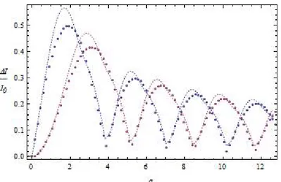
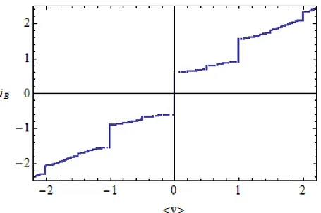
For the TBJJ, a four layer superconducting system, in which the inner two superconducting layers are treated as pure quantum mechanical systems, the coupling constants between the layers 1-2, 2-3 and 3-4 are different, so also in this case we have non-homogeneous couplings, and the coupling constants between 1-3 and 2-4 are considered smaller than the previous ones. For sake of simplicity, we take the superconducting phase difference of the inner layers 2 and 3 equal to zero. Under these hypotheses, by using Ohta’s semi-classical model, we have obtained the current phase relation (CPR) for these systems. It is seen that these devices are different from the sinusoidal one, characterizing the simple Josephson Junction (SJJ), and is in good agreement both with the theoretical results obtained by Brinkmann, based on a microscopic approach, and also with the experimental results found by Nevirkovets et al. The latter results are based on the observation of the Shapiro steps, and the analysis of their amplitudes as a function of the applied voltage.
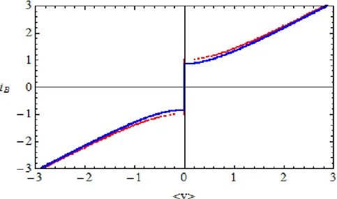
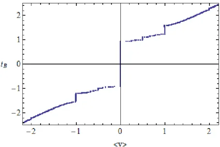
The voltage- current characteristics of a TBJJ, with the previously considered properties, have been analytically and numerically studied, both in the case of homogeneous coupling between all the superconducting layers and also in the non-homogeneous one. In the homogeneous case, and considering also a constant bias of electric current, the voltage-current characteristic of a TBJJ has an analytic form very similar to the one of a SJJ, despite a TBJJ has a non-canonical CPR. Of course, in the case of a TBJJ, we have an opportune value of the constant of normalization for the current, which is different from the corresponding value for a SJJ.
However, in the case of inhomogeneous coupling between different layers in the TBJJ, we obtain a deviation from this behaviour. In the presence of a radio frequency radiation, integer and fractional Shapiro steps are predicted, whose amplitudes, calculated in the homogeneous case, are a clear indication of the non-canonical CPR of these systems.
After these theoretical remarks about Josephson Junctions, we describe a mechanical analogy between a Josephson Junction and a simple pendulum, in the over-damped limit. This condition, in the case of a simple pendulum, indicates that the medium is characterized by a large value of the coefficient of viscosity, while, in the case of a Josephson Junction, denotes negligible capacitive effects between the two superconducting electrodes. In this situation, we have found that the dynamical equation of a simple pendulum is formally equivalent to the one of a Josephson Junction. This mechanical analogy can also be used for didactical purposes in order to grasp further information about the voltage- current relation of over-damping Josephson Junctions.
A further topic treated in the present work has been the semi-classical and quantum analysis of one-junction and two-one-junction quantum interference devices. These systems consist of a superconducting loop interrupted by one or two Josephson junctions. Starting from a review of the semi-classical and quantum properties of one-junction interference devices, we have extended our analysis to two-junction interferometers. In particular, we have determined the Hamiltonian function for this system in the semi-classical limit, and the Hamiltonian operator in the corresponding quantum case limited to a Hilbert space spanned by the flux number kets and . In the condition of a negligible value of the superconducting loop inductance, we have also calculated, in the quantum regime, the energy and the electric current for these two representative states.
As for the second part of the PhD thesis accomplished with the collaboration of the Russian professors mentioned before, the application of superconductor devices, in particular of SQUIDs, as detectors of Dark Matter has been analysed. In this way, an introduction of the problem of Dark Matter in the modern cosmology has been given. In particular, two important experiments for the registration of Dark Matter particles, one based on Josephson Junctions and the other one based on the use of SQUID, have been analysed. The first experiment uses a multi-channel detector, made up by a set of weakly coupled superconductors, so that they form a system of Josephson Junctions, displaced in the geometrical form of a matrix. The second experiment is a system made up by a paramagnetic calorimeter connected with a SQUID, by which it is possible to register the rate of interaction of Dark Matter particles, and also the energy release with the atoms of the material. In fact, there are several modes of operation of this experimental apparatus, and in particular we have focused on the dual channel mode of operation, in order to reduce the lepton background noise corresponding to the registration process.
After these considerations, we have dedicated to the analysis of the possible creation of a magnetic moment for Dark Matter particles: if they possess this magnetic moment they can electromagnetically interact with the common matter, and we have calculated that the cross section of this interaction is 9 orders of magnitude larger than the contact interaction with the atomic nucleus.
We have also overviewed a theoretical model exploring the possibility that Dark Matter and Dark Energy are two aspects of the same Cosmological Essence, defined “Dark Substance”. According to this theoretical model, Dark Energy represents the unperturbed state of Dark Substance, while Dark Matter particles play the role of swings or perturbations of it. These perturbations will be stable if all their decay channels are blocked, and also, more interestingly for our case, if they are in their
state of lowest relative energy minimum, where they coincide with the particles we can experimentally register. In fact, the potential energy of the perturbed state of Dark Substance presents some positions of relative minimum, which act as traps for its metastable excited states. In these positions of relative minimum, the Dark matter particles are in an excited state, so instable, while in the lowest position of relative minimum they are stable, and so do not decay, according to the main property of Dark Matter particles. On the other hand, the position of absolute minimum is occupied by Dark Energy, as in this theoretical model Dark Energy represents the unperturbed state of Dark Substance.
We have finally described two types of experimental systems, which are suitable for Dark Matter registration in the two cases considered above. In particular, for the registration of Dark Matter into the form of particles, we propose use of a SQUID-paramagnetic absorber, while for the registration of a flux of Dark Matter, or equivalently, according to the theoretical model of Dark Substance, of a corpuscular flux of Dark Energy, we propose use of a SQUID-magnetostrictor.
Chapter 1
From microscopic to macroscopic description of
Josephson dynamics
In this chapter we consider a theoretical model, based on quantum mechanics, of the Josephson dynamics. In particular, we analyse an array of N coupled superconductors, in which we consider only the interaction between nearest neighbour sites. By using some properties of the quantum operators algebra, and the Heisenberg picture in quantum mechanics, we obtain a particular set of linear differential equations. With opportune considerations, we can adapt this description to only two coupled superconductors, and so we finally obtain two differential linear equations, which are similar to those derived by Feynman in his celebrated model for Josephson junctions.
1.1 Introduction
The dynamics of two weakly-coupled superconductors was first predicted by Josephson in 1963 [1]. Successively, a simple and celebrated model of a Josephson junction (JJ) was proposed by Feynman [2]. Even though Feynman’s description of a JJ is useful in considering a two-level quantum system in which the interacting condensates are not perturbed by an external classical system, the case in which an external voltage source is applied across the JJ has been fully taken into account by Ohta [3]. In this respect, an analysis taking from a microscopic Hamiltonian to the Feynman equations for a Josephson junction is still lacking. More recently, after the discovery of high-temperature superconductors [4], models of one-dimensional arrays of Josephson junctions [5-7] have been widely adopted in the study of the physical properties of granular superconducting systems.
In the present chapter we perform a microscopic analysis of N coupled superconductors in which nearest-neighbour interactions are present. We define the dynamics of the order parameter of each superconducting element by recurring to the Heisenberg picture for fermionic operators. In this way, a set of coupled ordinary differential equations (ODEs) is obtained. When specializing this system of ODEs to only two coupled superconductors, Feynman’s model can be obtained. These results confirm the correspondence between the microscopic picture proposed in the present chapter and, by generalizing to a non-isolated JJ, the semi-classical analysis given by Ohta. In this way, further generalization of Ohta’s model to multi-barrier Josephson junctions [8] based on the semi-classical analysis can be retained to agree with a strict microscopic description of these types of junctions, lately proposed for application in fabricating innovative quantum interference devices [9-10].
1.2 Feynman’s model
In this section, we consider Feynman’s model and Ohta’s semi-classical model [2], [3], for the description of the dynamics of a Josephson Junction JJ, (i.e. a system made up by two weakly coupled superconductors, S1 and S2), that is based on the Josephson’s equations:
dt d V sen I I J 2 0 0 , (1.1)
where I is the superconducting current flowing through the insulating barrier, IJ,0 being its
maximum value, 2 1 is the superconducting phase difference across the JJ, in which and 1 2
are the superconducting phases of the k-th electrode, V is the voltage drop through the JJ, and
e h 2
0
is the elementary flux quantum, expressed as the ratio of Planck’s constant h, and of the absolute value of the Cooper pair charge 2e.
We start by noticing that the superconducting phases and 1 are defined in the wave functions of 2
the considered superconductors: 2 1 2 2 1 1 ; N ei N ei , (1.2)
where N is the number density of Cooper pairs. We can sketch a Josephson junction in the next k
figure 1.1.
Figure 1.1. A Josephson junction. This device is made up by two pieces of superconducting
materials, separated by a very thin insulating barrier.
The Feynman’s model [2] is a pure quantum mechanics model, which is able [11] to derive only the first of the equations (1.1), the so called Current-Phase Relation (CPR), but it is not able to derive the second one, that is called Voltage-Frequency Relation (VFR). In fact, it does not provide a consistent account of the external bias circuit, which has a parallel connection with the JJ, as shown in figure 1.2.
This drawback was solved by Ohta [2], [3], who introduced a semi-classical model based on a rigorous quantum derivation, in which an additional term, due to energy contribution of the external classical circuit biasing the JJ, is added. Let us consider, the analytic description of these two models.
Starting with Feynman’s model, which is, as just said, a quantum mechanical model, we can describe [11] the dynamics of JJ by using the Schroedinger equation:
0 ˆ H t i , (1.3) where 2 1
and and 1 have been defined in equation (1.2). 2
Figure 1.2. A schematic representation of Josephson junction with both electrodes connected to an
external classical circuit.
We can calculate the matrix expression of the Hamiltonian operator Hˆ0; it is made up by the summation of three terms:
K H H H
Hˆ0 ˆ1 ˆ2 ˆ , (1.4)
where H ˆ1 E11 1 is the Hamiltonian operator of the superconductor 1, H ˆ2 E22 2 is the Hamiltonian operator of the superconductor 2, and HˆK K (1 2 2 1 ) is the Hamiltonian operator describing the interaction between the two superconductors. By considering that the vectors 1 and 2 constitute an orthonormal set, we know that:
j i for j i for j i j i 0 1 , (1.5)
So, if we calculate the matrix elements of the operator Hˆ0:
j i for K j i for E H Hˆ0)ij i ˆ0j i (
we get: 2 1 0 ˆ E K K E H . (1.6)
By now substituting (1.6) in (1.3), and making the matrix product, we have:
2 1 2 1 2 1 E K K E t i 1 2 2 2 2 1 1 1 K E t i K E t i (1.7)
If we express the scalar wave functions as in (1.2), we get, from the first equation: 2 1 1 1 2 1 1 1 1 1 1 2 i i i i e N K e N E dt d e N e dt dN N i .
If we now multiply both members by
1 1 N ei , we obtain: i e N N K E dt dN N i dt d 1 2 1 1 1 1 2 , (1.8)
where 21 is the superconducting phase difference. By doing the same for the second equation, in particular, by multiplying both members of the second equation by
2 2 N ei , we obtain: i e N N K E dt dN N i dt d 2 1 2 2 2 2 2 . (1.9) By expressing sin cos i ei , from (1.8), we get: sin cos 2 1 2 1 2 1 1 1 1 N N K i N N K E dt dN N i dt d . (1.10)
sin 2 cos 1 2 1 1 1 2 1 1 N N K dt dN N N N K E dt d
In the same way, from the expression:
sin cos 2 2 1 2 1 2 2 2 2 N N K i N N K E dt dN N i dt d (1.11) we get: sin 2 cos 2 1 2 2 2 1 2 2 N N K dt dN N N N K E dt d Therefore, we obtain: dt dN N N K N N KN dt dN 1 2 1 2 1 2 2 sin 2 sin 2 .
The relation 2 1 2K N1N2sin
dt dN dt dN
satisfies the principle of charge conservation, since we can interpret the term 2eNi with i = 1, 2 as the electric charge density for unitary volume inside the i-th superconductor, and so the time variation of it represents the electric current flowing from a superconductor to the other one. Therefore, by multiplying the equation
sin 2 2 1 2 N N K dt dN
by the term -2e in both members, we obtain:
sin 0 , j I I , where dt eN d I (2 2)
which is the electric current, made up by Cooper pairs, flowing between the superconductors, and IJ,0 4eK N1N2
.
In this way, we notice that, by using the Feynman model, we have obtained the first Josephson equation, i.e. the CPR. This means that the Feynman model is able to describe the CPR of a Josephson junction.
As far as the second Josephson equation (i.e. the VFR) is concerned, we can consider that, by subtracting from the expression of
dt d2
the one of dt d1
. cos ) ( ) ( cos cos ) ( 1 2 2 1 1 2 1 2 1 2 1 2 1 2 1 2 N N N N K E E dt d N N K E N N K E dt d
By taking 2 1 and E2 E12eV we finally obtain:
cos 2 1 2 2 1 N N N N K eV dt d . (1.12)
In order to obtain from this equation the VFR, we must have that N 1 N2; this latter relation, however, is not consistent with conservation of electric charge N1 N2 0. Therefore, we may conclude that the Feynman model does not provide a proof of the strict voltage-frequency Josephson relation (VFR). The importance of Feynman model, however, rests in the fact that a single JJ can be considered, at least in first approximation, as an isolated quantum system, which verifies the current-phase relation (CPR). Furthermore, Feynman’s model can be applied to any weakly coupled two-level quantum system as long as it does not interact with the classical world.
1.3 Ohta’s semi-classical model
In his important work [3], Ohta stated that he had long been puzzled by the fact that one could not achieve a strict VFR by means of the Feynman model. He thus developed a rigorous semi-classical analysis which took into account the contribution due to the external circuit. We shall here give a simplified account [11] of the more complete analysis given by Ohta.
Starting from quantum mechanical considerations, Ohta first recovered Feynman’s Hamiltonian. However, considering the classical nature of the problem (the system made up by the external circuit and the JJ), Ohta projected Feynman results onto the classical world. A way to do this is to consider the classically observable energy:
0
0 Hˆ
H . (1.13) Carrying out the calculations, we find:
. 2 2 ) ( ) ( 2 1 2 2 1 1 ) ( 2 1 ) ( 2 1 2 2 1 1 2 1 2 1 2 2 2 2 1 1 2 2 2 2 1 2 1 1 1 1 2 1 2 1 2 1 0 1 2 1 2 1 2 1 2 i i i i e e N N K N E N E e N N K e N N K N E N E K K E E E K K E E K K E H So, we get: ) cos( 2 1 2 2 1 2 2 1 1 0 E N E N K N N H . (1.14)This is only one portion of the classical Hamiltonian related to the whole system in figure 1.2. The remaining portion is given by the energy provided by the circuit, which can be written as
IVdt
W , typical form of an electromagnetic energy. In this way, the classical complete Hamiltonian can be written as follows:
W N N K N E N E W H H 0 1 1 2 22 1 2 cos(21) . (1.15)
The minus sign near the expression for W is due to the fact that it represents an energy transferred from the external environment to the system.
The transition to the classical world is, in this way, complete so that a solution to the problem by classical mechanics can be found. First, let us note that and k Nk are conjugate variables (angle-action variables, for k = 1, 2). Hamilton’s equations thus give:
k k H N (1.16a) k k N H 1 (1.16b)
for k = 1, 2, where the dot represents the time derivative.
By now defining the coupling energy as EC 2K N1N2 cos(2 1), and by setting
W E
ER C , (1.17) we may rewrite the above equations as follows:
k R k E N (1.18a) k R k k N E E 1 (1.18b)
for k = 1, 2. Let us now consider the time derivative of E ; by using the theorem of total R differential we get:
2 1 k k k R k k R R E N N E E . (1.19)By using the relations (1.18a) and (1.18b), we obtain:
2 1 2 1 2 1 ) ( 1 1 k k k k k k k R k R k k R k R k R R E N E E N E E E E N E E . So we get:) ( ) ( 1 1 2 2 2 1 N E N E E N E k k k R
.If we set E1 eV and E 2 eV, so that E2 E1 2eV, we find:
E dt E N E N E N E N dt eV N N dt ER R ( 1 1 2 2) ( 1 1 2 2) ( 2 1) . (1.20)Let us now consider the Josephson Junction to be in a thermal bath, which is the condition indicating that the temperature is uniform and constant in all the thermodynamic system considered, so that N1 N2 0. In this way, the charge conservation relation N1 N2 0 becomes a trivial
identity and the function E is seen to be zero. We may also notice that, for constant values of R E 1
and E , the Hamiltonian H is a constant of motion, so that the energy of the system is conserved. 2
By using these results, in particular the relation (1.18b), we have:
k k E (1.21) for k = 1, 2. This relation leads directly to the VFR, in fact, by knowing that
E2 E1 2eV 1 2
and by denoting by 21 the difference between the superconducting phases of the electrodes in the Josephson Junction, we obtain:
2eV
. (1.22) The above expression is the strict form of the VFR sought.
In addition, if we look in details at the condition of thermal bath, according to which 0 0 R R E E , we have: IV N N K W EC 2(21) 1 2sin(21) By using the relation (1.22) we get:
sin 4 2 1N N eK I . (1.23) Equation(1.23) is just the CPR for a Josephson Junction, expressed in the relation (1.1).
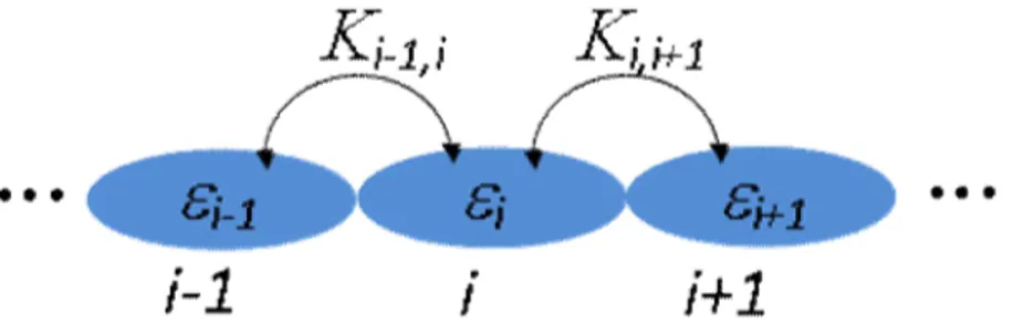
1.4 N coupled superconductors
In order to prove that Feynman model indeed follows from a microscopic analysis of the superconducting system, we can start by considering [12] the Hamiltonian operator Hˆ for an array
.) . ˆ ˆ ( .) . ˆ ˆ ( ˆ ˆ ˆ , , , 1 1 , , , , , , c c c hc K c c hc c H i i i i i i i i i i i i i
, (1.24)where i = 1, 2, …, N is the index labelling the superconductors, is the spin index, which assumes
only the two values , (spin up and spin down), Ki, i 1 is the coupling constant between the
superconductors i and i+1, which describes the electromagnetic interaction between two electrons, each one in a different site (i or i +1), cˆ and cˆare the operators of destruction and creation, and h.c. stands for hermitian conjugate. For example, the hermitian conjugate of the operator ˆ,ˆ,
i i ic c is the operator *ˆ,ˆ, i i
ic c , in which, by the symbol * we denote the complex conjugate of a function or of a constant. In the same way, the hermitian conjugate of the operator Ki,i1cˆi1,cˆi, is the operator: * , 1, 1 , ˆ ˆ i i i i c c
K . In these expressions we have also considered the term , defined in the i following way : i , , ˆ ˆi ci c . (1.25)
The quantity is thus the time dependent expectation value of the product of two destruction i operators. This quantity can be identified with the order parameter, being it proportional to the numerical density of Cooper pairs.
We can sketch this system, and the interactions among its superconductors in the next figure 1.3.
Figure 1.3. Schematic representation of a one-dimensional array of weakly coupled
superconducting islands. The coupling constant between the adjacent sites i and i+1 is denoted by Ki,i+1.
The Hamiltonian operator written in (1.24), which can act on the superconducting wave function of a single electron on the site i, for i = 1,2, …, N, is made up by the sum of three terms (that are three summations).
The first term, Hˆ0
, , , ˆ ˆ i i iic c , as usual, describes the kinetic properties of electrons. The scalar quantity is the energy of an electron; so the analytic expression of i Hˆ0 represents the total
kinetic energy of the electrons present on the N superconductors.
The second term, denoted as HˆS, describes the coupling potential energy of a single pair of electrons, both present on the same superconductor, represented by the index i, (it’s well known, in the theory of superconductivity, that these electrons, through their electromagnetic interaction with
the ions of lattice, become a Cooper pair). By carrying out the summation on all the N superconductors, we get all the possible interactions between the electrons present on each of these superconductors, as represented by the analytic expression of H . S
The third term, denoted as HˆK, describes the interaction potential energy between electrons on next neighbouring superconductors. In the analytic expression of HˆK, we notice that Ki, i 1 is the
coupling constant between two next neighbouring superconductors (i and i+1), the operator cˆi1,
creates an electron on the superconductor i+1, and the operator cˆi, destroys an electron on the superconductor i; in the same way, the hermitian conjugated operator h.c., defined before in expression (1.24), destroys an electron on the site i+1 and creates it on the site i. So, an electron is induced to pass (or we may say to jump) from a superconductor to the next one, and for this reason, the term HˆK can be defined “hopping term”. It is interesting to notice that one could arrive to a similar analytic expression of the Hamiltonian by considering a Fermi- Hubbard model with an attractive interaction [13], and also by a mean-field approximation giving the definition of the order parameter in (1.25).
Once we have described [12] the analytic properties of the Hamiltonian operator Hˆ , let us
consider the time evolution of the function , which, as just considered, can be interpreted as the i wave function of the superconducting state on the site i. In order to analyse the time evolution of i
this quantity, for which :
c H
c t i ˆi, ˆi,, ˆ . (1.26)For sake of simplicity, we can denote the symbol t
as . t
The fermionic operators cˆi, obey to the following anti-commutation rules:
ˆ, ,ˆ , '
0 ;
ˆ ,ˆ , '
' ;
ˆ, ,ˆ , '
0 j i j ij i j i c c c c c c . (1.27) So, we get:
c H
c i c
c H
i c c i i t i t ˆi, ˆi, ˆi, , ˆ ˆi, ˆi, ˆi, , ˆ . (1.28) By using the relations (1.27), and the property:
Aˆ,BˆCˆ
Aˆ,Bˆ CˆBˆ
Aˆ,Cˆ we can calculate the two terms
cˆi,,Hˆ
and
cˆi,,Hˆ
.Therefore, knowing that Hˆ Hˆ0 HˆS HˆK we get:
ˆ,, ˆ0
ˆ, ;
ˆ,, ˆ
(ˆ, , ˆ, ,) ;
ˆ,, ˆ
1, ˆ1, 1, ˆ1, i i i S i i i i K i i i i i i i H c c H c c c H K c K c c (1.29)where ,.
By using these results for the operators of commutation, and by doing all the calculations, inside (1.28), if we consider the operators
ˆ, ˆ, ˆ, ˆ, ˆ i i i i i c c c c n (1.30) and the functions
i cˆi, cˆi 1, cˆi1, cˆi, (1.31) we get the equations:
i
i i i i i i i i i i t n K K i 2 12 ˆ 1,1 1, . (1.32) In all these expressions i = 1, 2,…, N. In order to define the complete dynamics of the system of theN differential equations in (1.32), we need to define the time evolution of the functions defined in
(1.31), and so we calculate:
c H
c c
c H
c H
c c
c H
iti ˆi,, ˆ ˆ11, ˆi, ˆi1,, ˆ ˆi1,, ˆ ˆi, ˆi1, ˆi,, ˆ . (1.33)
By using the relations (1.29), and by getting out all the calculations, we obtain:
1 1 , 2 , 1 1 , 1 * 1 , 1) ( 2 ) ( 2 ) ( t i i i i Mi Kii i Mi Ki i i Ki i i Ki i i i (1.34)
where we have defined the following functions:
, , 1 , , 1 * , 1 , , 1 , ˆ ˆ ˆ ˆ ˆ ˆ ˆ ˆ i i i i i i i i i i c c c c M c c c c M (1.35)
and the function as follows: i
i cˆi 1, cˆi1, cˆi 1, cˆi 1, . (1.36) According to our hypothesis of interactions only between first neighbouring sites, the next neighbouring sites are uncorrelated, and so we have i 0. In this way, equations (1.20) and (1.22) suffice to describe the dynamics of the system of N coupled superconductors.
In the following section we shall consider the application of these results to the case of 2 coupled superconductors, which form the so called Josephson Junction, and we solve, by using some approximations, the equations (1.20) and so also the equations (1.22).
1.5 Two coupled superconductors: a Josephson Junction
In the case of only two coupled superconductors (N = 2), we may rewrite [12] equations (1.32) and (1.34) by considering i = 1, 2. We can also show that the expectation value of the number operator
ˆ, ˆ, ˆ, ˆ, ˆ i i i i c c c c n is n 2 1
. In fact, we can consider that electrons are fermions, so they obey to the Fermi-Dirac statistics, that is:
T k E B e E f 1 1 )
( ; as the chemical potential is very close to
Fermi energy E , and the most sensible electrons to the interaction with phonons (so that Cooper F
pairs are formed) are the ones whose energy is closest to the Fermi energy E , we notice that, for F these electrons: 2 1 ) ( ) (E f EF f . (1.37)
It is known that the Fermi-Dirac statistics represents the number of fermions per unitary volume, in an unitary range of energy values, we notice that this number is
2 1
. As the expectation value of the number operator equals to the number of particles which are present in a well defined state (0 or 1, according to Pauli Exclusion Principle), it can be considered equals to the number of electrons represented by the Fermi-Dirac statistics,
2 1 ) (EF
f .
So, we may set
2 1 2 1 n n n . (1.38)
Thus, in the case of N = 2 coupled superconductors, we have, from equations (1.32) and (1.34):
2 2 , 3 1 1 2 2 2 2 1 , 2 * 1 1 2 , 1 1 1 2 1 1 1 1 , 2 0 0 1 1 1 1 2 ) 2 ( ) 2 ( ) ( ) 2 1 2 1 ( 2 K K i K M K M i K K i t t t
As we are only considering two superconductors, we have: K3,2 0. We can also set K
K
K1,2 2,1 , and make use of the simplifying hypothesis by which 1 * 1 M
M , so that M is a 1
real function of time. In this way, the previous set of differential equations can be simplified as follows: 1 2 2 2 2 1 1 1 2 1 1 1 1 1 1 2 ) )( 2 ( 2 ) ( 2 K i M K i K i t t t (1.39)
In order to solve [5] the two differential equations for and 1 , we can solve the differential 2
equation for ; so, substituting the analytic expression obtained for 1 inside the differential 1
equations for and 1 , we can solve them. As for the solution of the differential equation for 2 , 1
we can, first of all, set:
eV eV M K K 1 2 1 ; ; 2 ~ (1.40) So we have: 1 2 .
In this way, the differential equation for can be rewritten in the more simplified form: 1
) ( ~ 2 2 1 1 2 1 K i t . (1.41)
Being it a linear differential equation, we know that its more general solution can be expressed as the sum of the solution of its homogeneous associated differential equation, and of a particular solution of (1.41). The associated homogeneous differential equation is:
0 )
2
(it 1,H , its solution being:
) 2 exp( ) 0 ( ) ( 1 , 1 t i t H . (1.42)
In order to find the particular solution of (1.41), we can use the method of Green function:
2 ' ' ' 1 ' , 1 ( ) ( ) ( ) ~ 2 ) (t K t t t t dt P (1.43)in which (t) is the Green function, or also called the kernel function, and must satisfy this differential equation: ) ( ) ( ) 2 (it t t (1.44) where (t) is the Dirac distribution function, so defined:
0 0 0 ) ( t for t for t (1.45)
In fact, if we substitute the expression (1.43) in (1.41), and, by using the expression (1.32), we do all the calculations, we find this result:
2 ) 2~ ( ) ( ) ( ) 2~( ( ) ( )) (i t 1,P K t t' 1 t' 2 t' dt' K 1 t 2 t ,where, in the latter equation, we have used the property (1.45) of Dirac distribution function. Having found that (1.43) is a particular solution of (1.41), we must determine the analytic expression of the function (t); it can be expressed in the factorized form:
) ( ) ( ) (t At t (1.46) where (t) is the Heaviside unitary step function, so defined:
0 0 0 1 ) ( t for t for t
The reason why we use this function, inside the expression (1.46), is that (t) represents the response of the system to an external interaction, represented by the function (1.45); in particular, this response starts at t0, and it is zero before, i. e., for t < 0. Therefore, by inserting the expression (1.46) inside (1.44), and by doing the opportune calculations, we get:
( ) 2 ( )
1 (0)
( ) ) ( ) ( ) ( ) ( ) ( ) ( 2 ) ( ) ( t A i t A t A i t t t t A i t A t t A i t t t t (1.47)In this expression we have used the result: ) ( ) ( t dt t d (1.48) so that ( ) i A(t) (t) dt d t A
i , and, by using the property of (t) that, for t0 is equals to 0, we have: ) ( ) 0 ( ) ( ) (t t i A t A i .
As A(0) is an arbitrary constant, we can take:
i A(0) .
So, the equation (1.24) becomes:
( ) 2 ( )
0 )(t i tAt A t
.
Knowing that, for t0 (t)1, we get: 0 ) ( ) 2 (i A t (1.49)
and its solution is: ) 2 exp( ) (t i i t A . Therefore: ) ( )exp 2 ( ) (t t' i t t' i t t' (1.50) and
' ' ' , 1 ( ) 2 exp ) ( ~ 2 ) (t iK t t i t t dt P . (1.51)As we have just said, the most general solution of (1.51) is given by the sum of the solution of the homogeneous associated differential equation, and of the particular solution considered:
) ( ) ( ) ( 1, 1, 1 t H t P t . (1.52)
For ranges of time t >> 0 we can consider negligible the term 1,H(t), and so we can approximate the solution with 1,P(t)1(t)1,P(t) for t >> 0. In order to simplify the expression (1.51), we can, first of all, notice that for tt' 0tt' we have:
1 ) (t t'
,
while for t t' 0 we have: (t t')0. Therefore, we can rewrite the (1.51) in the following way:
t dt t t i t t K i t 2 ' ' ' ' 1 1 ( ) 2 exp ) ( ) ( ~ 2 ) ( . (1.53)To further simplify this expression, we can operate [12] the following change of variables:
2
i . (1.54) So, in the expression of the exponential function, we get:
2 ( ) exp 2 ( ) exp ( ) exp i t t' i t t' t t' . In this way the expression (1.53) becomes:
t dt t t t t i t t K i t 2 ' ' ' ' ' 1 1 ( ) exp ( ) 2 exp ) ( ) ( ~ 2 ) ( (1.55)where we have considered for sake of simplicity. The position (1.54) allows the introduction of a cut-off time t in the expression (1.55). In fact, for * t sufficiently close to t, we may set: *
t t t t t dt t t t t i t t K i dt t t t t i t t K i dt t t t t i t t K i t * * * ' ' ' ' 2 ' 1 ' ' ' ' 2 ' 1 ' ' ' ' 2 ' 1 1 ) ( exp ) ( 2 exp ) ( ) ( ~ 2 ) ( exp ) ( 2 exp ) ( ) ( ~ 2 ) ( exp ) ( 2 exp ) ( ) ( ~ 2 ) ( where we can consider negligible the first integral, because for t comprised between ' and t *
we have: 1 ) ( exp ' t t
so that the first integral tends towards zero.
Assuming now that 1(t) and 2(t) are slowly varying functions in the interval
t ,t * , we get:
t t dt t t t t i t t K i t * ' ' ' 2 1 1 ( ) exp ( ) 2 exp ) ( ) ( ~ 2 ) ( . (1.56)In this way, we can calculate the integral considered in (1.56) as follows
t t t t dt t t i dt t t t t i * * ' ' ' ' ' 1 exp ) ( 2 exp ) ( exp ) ( 2 exp .In fact, as t is very close to ' t , it is possible to approximate * t with t' t t* , and we can set:
A A t t A exp 1 exp ) ( exp ' . The relation
A , with A a constant of order one, follows from the fact that is the potential
interaction energy between two electrons, one on the site i, and the other one on the site i +1, which decays in a characteristic time . We can also consider that the interaction energy is usually less
than the energy of an electron on the site i; in reality it happens that the electrons forming a
Cooper pair, and belonging to different first neighbour sites, tend to pass on the same site, so to lead to the creation of Cooper pairs on the same superconductor site. In this way, we can say that expression (1.55) indicates the sum of the kinetic energy of the electron (represented by ), plus i
the interaction energy of the same electron with the external environment, that in this case is the
next-neighbour superconductor, is the total energy of the electron. The factor 2 in (1.55) is taken in order to simplify the calculations in expression (1.56).
Coming back to the calculation of integral in (1.56), we may consider that the term A exp can
be directly inserted inside the constant K~. In this way, we can calculate the integral as follows:
t t t t t t t i i t t i i t t i * * ' ) ( 2 exp 1 2 ) ( 2 exp 2 ) ( 2 exp ' ' * .By noticing that tt* 1, we can approximate the exponential term as:
2 2 2 1 2 1 2 exp i i i
having considered the Taylor series expansion of
2 1
2
x x
ex valid for x << 1. In this way, considering the expression (1.56), we get:
( ) ( )
2 1 2 ~ 1
( ) ( )
. ~ 2 2 1 2 1 1 2 ) ( ) ( ~ 2 ) ( 2 1 2 1 2 2 1 1 t t i K i i i t t K i i i t t K i t If we substitute this expression obtained for 1(t) inside the two differential equations for and 1 2
, in the expression (1.39), we get for 1:
( ) ( )
1 ~ 2 2 1 1 1 2 1 t t i K iK i t . (1.57) By setting: i K iK 1 ~ 2 (1.58) we get: 2 1 1 1 1 2 t i it1 (21)1(t)2(t). In the same way, we get, for : 21 2 2 2 (2 ) t i . By now setting i i E 2 , (i1,2)
where E can be interpreted as the energy of the Cooper pair ( so a system of two electrons) on the i
superconductor i, we obtain the following form for the differential equations:
1 2 2 2 2 1 1 1 ) ( ) ( E i E i t t (1.59)
In order to obtain an Hamiltonian system, as in the case of Feynman’s celebrated model of Josephson Junctions, we can consider that in (1.58) there is a real part, defined as , and an R imaginary part, defined as . In this respect, we notice that the quantity I = R 2
2 ~ 2 KK is a real parameter, describing the interaction energy between two Cooper pairs on different superconducting sites. In fact, we know that is proportional to R
1, where , defined in expression (1.54), is,
as just considered, the potential energy between two electrons on different first neighbour sites. By considering the quantities Ek EkR
~
, which are the effective energies of a Cooper pair on the site k = 1, 2, we get: 1 2 2 2 2 1 1 1 ~ ~ R t R t E i E i (1.60)
These differential equations are similar to the ones obtained by Feynman in his celebrated model of a Josephson junction. At the end of this chapter we may notice that, in deriving equation (1.60), we have made use of a formal solution of in terms of 1 and 1 , as expressed in relations (1.39). If 2
we carry out the same kind of analysis for more than two coupled superconductors, we can obtain the extension of Feynman’s and Ohta’s models to multi-barrier Josephson junctions, already proposed by De Luca and Romeo in reference [14], which is, as just remarked in the introduction, in good agreement with a strict microscopic description of these types of devices.
1.6 Conclusions
We have considered a microscopic description of N coupled superconductors in which nearest-neighbour interactions are present. Starting from the time evolution of the fermionic operators cˆ
and
cˆ in the Heisenberg picture, we obtain a set of coupled ordinary differential equations for the order parameters i.
Since the main aim of the present analysis is to show that Feynman’s model for a single Josephson junction can be justified by a microscopic model, we have specifically written the resulting system of differential equations in the case of two coupled superconductors. In this simple case Feynman’s model is obtained. In this way, one can argue that there exists a strict correspondence between the microscopic picture described in the present work and the semi-classical analysis proposed by Feynman and successively refined by Ohta. Therefore, generalizations of Ohta’s model to multi-barrier Josephson junctions [8] based on the semi-classical analysis developed by the latter authors can be retained to agree with a strict microscopic description of these systems.
Chapter 2
Mechanical analogue of an over-damped Josephson
junction
An over-damped pendulum can be adopted as a mechanical analog of an over-damped Josephson junction. The basic equations leading to the driving torque versus the time average of the angular frequency are studied. The mechanical analog can be used to provide additional insight into the current-voltage characteristics of over-damped Josephson junctions.
2.1 Introduction
In 1973 B. D. Josephson received the Nobel Prize for having predicted the so called d. c. and a. c. Josephson effects [1] in a superconducting device that was named after him: the Josephson junction (JJ). A JJ consists of two weakly coupled superconductors. The dynamics of the superconducting phase difference across the junction is described by the following equations [15]:
sin 0 , J I I (2.1a) eV dt d 2 (2.1b)
where I is the current flowing through the junction (IJ,0being the maximum value that can flow inside the zero-voltage state), ħh, h being Planck’s constant, and V is the voltage across the
two superconductors.
In the d. c. Josephson effect a non-dissipative current can be seen to flow at zero voltage, as it can be shown by setting V=0 in (2.1b), so that constant. In this way, IJ,0 represents the maximum
value of I flowing in the junction in the zero-voltage state.
In the a. c. Josephson effect, the voltage across the JJ is kept at a fixed non-zero value V0.
Integrating both sides of Eq. (2.1b) we obtain (t)eħVt 0where is the constant of 0
integration. Therefore the current I is seen to oscillate at a frequency J eħV.
Alternative derivations of equations (2.1a-b) have been also proposed by Feynman [2] and by Ohta [3], as we have seen in the preceding chapter. In the Feynman model a JJ is described as a weakly coupled two-level quantum system. Ohta noticed that Feynman model did not include an additional term due to energy contribution of the external classical circuit biasing the Josephson junction. The latter author therefore introduced a semi-classical model based on a rigorous quantum derivation to attain full agreement between equations (2.1a-b) and the corresponding final equations obtained by means of his valuable semi-classical analysis.
In order to describe the dynamics of the superconducting phase difference in an over-damped
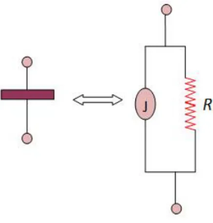
Figure 2.1. Resistively Shunted Model for a Josephson junction. The junction on the left is
described by a parallel connection of a resistor with resistance R and an ideal Josephson element J. In the latter a current I IJ,0sin can flow.
In this model a purely superconducting element carrying a current I expressed in terms of as in
Eq. (2.1a) is placed in parallel with a resistor of resistance R, as shown in fig. 1. By injecting a current IB in the system and by invoking charge conservation, we may write:
B J I I R V ,0sin (2.2)
where V is the voltage across the JJ. By expressing V in terms of as in Eq. (1b) and by
introducing the dimensionless quantities
0 , J B B I I i and RIJ t 0 0 , 2
we may rewrite equation (2.2) as follows: B i d d sin . (2.3)
The above equation also represents [16] the dynamics of an over-damped simple pendulum. Therefore, starting from this analogy [15], [2], [3], [17], we consider the static and dynamic solutions of Eq. (2.3) referred to a simple pendulum with a constant forcing term, trying to grasp some physical insight from these expressions. Successively, we derive [16] the curve of the driving torque versus the time average of the angular frequency. Finally, the analogy between the two systems is utilized to discuss the current-voltage characteristics of over-damped Josephson junctions.
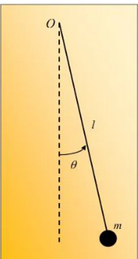
2.2 An over-damped pendulum
Let us consider [16] the pendulum hinged in O and consisting of a massless rod of length l and a spherical body of mass m, as shown in fig. 2.2. Let us also assume that the sphere of mass m has radius R. This sphere is moving in a fluid of density , so that it is subjected to the buoyance F
R