FISSICU platform on CRESCO-ENEA grid for thermal-hydraulic nuclear engineering

Titolo

FISSICU

platfo

rm on CRESCO-ENEA grid far

thermal-hydraulic nuclear engineering

Ente emittente CIRTEN

PAGINA DI GUARDIA

Tipologia del documento: Rapporto Tecnico

Collocazione contrattuale: Accordo di programma ENEA-MSE: tema di ricerca "Nuovo nucleare da fissione"

Argomenti trattati: Reattori nucleari evolutivi Sicurezza nucleare

Reattori nucleari ad acqua

Termoidraulica dei reattori nucleari

Sommario

Il documento descrive l'istallazione della piattaforma di simulazione avanzata FISSICU (FISsione/SICUrezza) per la termoidraulica e fluidodinamica realizzata dal dipartimento DIENCA­ UNIBO sulla rete di calcolatori CRESCO-ENEA di Portici. La piattaforma contiene codici per la simulazione a diversi livelli (microscala, scala intermedia e di sistema) di componenti, sistemi e facility nucleari. Per simulazioni tridimensionali dirette la piattaforma contiene i codici TRJO U e SA TURNE. Per la scala intermedia si è implementato il codice NEPTUNE, mentre a livello di sistema è stata prevista l'implementazione del codice CATHARE. Il software SALOME è stato utilizzato per l'accoppiamento dei codici e la gestione di diversi strumenti di generazione mesh, come GMESH and SALOME MESH, e di visualizzazione come PARAVIEW. Una sintetica guida è stata inoltre introdotta nel documento per supportare gli utenti nell 'utilizzo dei codici della piattaforma e degli strumenti di generazione mesh e visualizzazione.

Note

REPORT PAR 2007 LPS.B - CERSE-UNIBO RL 1302/2010

Autori: F. Bassenghi, G. Bornia A. Cervone, S. Manservisi

Università di Bologna, Dipartimento di Ingegneria Energetica, Nucleare e del Controllo Ambientale (DIENCA)

Copia n. In carico a: NOME FIRMA NOME FIRMA 2 1

Lavoro svolto in esecuzione della linea progettuale LP5 punto B2 - AdP ENEA MSE del 21/06/07

Tema 5.2.5.8 – “Nuovo Nucleare da Fissione”.

CIRTEN

CONSORZIO INTERUNIVERSITARIO

PER LA RICERCA TECNOLOGICA NUCLEARE

ALMA MATER STUDIORUM - UNIVERSITÀ DI BOLOGNA

DIPARTIMENTO

DI

INGEGNERIA

ENERGETICA,

NUCLEARE

E

DEL

CONTROLLO

AMBIENTALE

-

LABORATORIO

DI

MONTECUCCOLINO

FISSICU PLATFORM ON CRESCO-ENEA GRID FOR

THERMAL-HYDRAULIC NUCLEAR ENGINEERING

CIRTEN-UNIBO RL 1302/2010

AUTORI

F. Bassenghi, G. Bornia, A. Cervone, S. Manservisi

DIENCA - UNIVERSITY OF BOLOGNA Via dei Colli 16, 40136 Bologna, Italy

FISSICU PLATFORM ON CRESCO-ENEA GRID FOR THERMAL-HYDRAULIC NUCLEAR ENGINEERING

September 1 2010

Authors: F. Bassenghi, S. Bna, G. Bornia, A. Cervone, S. Manservisi and R. Scardovelli

sandro.manservisi@unibo.it

Abstract. The FISSICU (FISsione/SICUrezza) platform for CFD thermal-hydraulics is set on the CRESCO-ENEA GRID cluster located in Portici. The platform contains codes for microscale, intermediate and system scale simulations for components of nuclear plants and facilities. For direct three-dimensional numerical simulations the platform contains codes such as TRIO_U and SATURNE. At intermediate scale the platform implements codes such as NEPTUNE and for system level CATHARE will be available soon. The platform contains the SALOME application for code coupling and a large number of mesh generators and visualization tools. All the codes run starting from mesh input files with common formats. GMESH and SALOME MESH are open-source refer-ence mesh generators that can be found in the platform together with conversion tools.

Contents

1 FISSICU platform organization 8

1.1 Multiphysics and Multilevel platform . . . 8

1.1.1 Multiphysics analysis . . . 8

1.1.2 Multilevel analysis . . . 10

1.2 CRESCO-ENEA GRID . . . 11

1.2.1 CRESCO infrastructure . . . 11

1.2.2 CRESCO access . . . 11

1.2.3 CRESCO-ENEA FISSICU Platform . . . 13

1.2.4 Submission to CRESCO queues . . . 14

1.3 FISSICU platform input/output formats . . . 16

1.3.1 Input mesh format . . . 16

HDF5 format . . . 16

XDMF format . . . 18

MED format . . . 21

1.3.2 Platform visualization . . . 25

PARAVIEW on CRESCO-ENEA GRID . . . 25

The PARAVIEW application . . . 26

Documentation . . . 27

2 SALOME 28 2.1 Introduction . . . 28

2.1.1 Code development . . . 28

2.1.2 Location on CRESCO-ENEA GRID . . . 29

2.1.3 SALOME overview . . . 29

2.2 SALOME on CRESCO-ENEA GRID . . . 30

2.3 SALOME platform modules . . . 31

2.3.1 Introduction. . . 31 2.3.2 KERNEL . . . 31 2.3.3 GUI . . . 32 2.3.4 GEOM . . . 32 2.3.5 MED. . . 32 2.3.6 MESH . . . 33 2.3.7 POST-PRO . . . 33

2.3.8 YACS . . . 33

2.4 SALOME file transfer service . . . 34

2.4.1 File transfer service inside a program . . . 34

2.4.2 Python file transfer service . . . 34

2.4.3 Batch file transfer service . . . 35

2.5 SALOME Mesh creation . . . 35

2.5.1 Import and export of mesh files in SALOME . . . 35

2.5.2 Mesh tutorial from SALOME documentation . . . 36

2.5.3 Tutorial: step by step mesh on CRESCO-ENEA GRID. . . 36

3 SATURNE 57 3.1 Introduction . . . 57

3.1.1 Code development . . . 57

3.1.2 Location on CRESCO-ENEA GRID . . . 58

3.1.3 SATURNE overview . . . 58

3.2 SATURNE dataset and mesh files. . . 58

3.2.1 SATURNE mesh file . . . 58

3.2.2 SATURNE dataset file . . . 59

3.3 SATURNE on CRESCO-ENEA GRID . . . 63

3.3.1 Graphical interface . . . 63

3.3.2 Data structure . . . 63

3.3.3 Command line execution . . . 64

3.3.4 Batch running . . . 65

3.4 SATURNE tutorial: a simple heated channel test . . . 66

4 TRIO_U 93 4.1 Introduction . . . 93

4.1.1 Code development . . . 94

4.1.2 Location on CRESCO-ENEA GRID . . . 94

4.1.3 TRIO_U overview . . . 94

4.2 TRIO_U on CRESCO-ENEA GRID . . . 94

4.2.1 How to start TRIO_U from console . . . 95

4.2.2 How to start TRIO_U from FARO . . . 95

4.2.3 How to interrupt TRIO_U . . . 95

4.3 Mesh, dataset and output files. . . 96

4.3.1 Mesh File . . . 96

Xprepro mesh format. . . 96

Gmsh mesh format . . . 96

Tgrid/Gambit mesh format . . . 96

SALOME MED format . . . 97

4.3.2 Dataset file . . . 97

4.3.3 Output files . . . 98

CONTENTS

5 NEPTUNE 110

5.1 Introduction . . . 110

5.1.1 Code development . . . 110

5.1.2 Location on CRESCO-ENEA GRID . . . 111

5.1.3 NEPTUNE overview . . . 111

5.2 NEPTUNE on CRESCO-ENEA GRID . . . 112

5.2.1 Graphical interface . . . 112

5.2.2 Data structure . . . 112

5.2.3 Command line execution . . . 113

5.2.4 Batch running . . . 114

5.3 NEPTUNE dataset and mesh files . . . 114

5.3.1 NEPTUNE mesh file . . . 114

5.3.2 NEPTUNE param file . . . 114

Special Modules . . . 117 Fluid&flow properties . . . 117 Input-output control . . . 117 Numerical schemes . . . 117 Scalar . . . 117 Boundary Conditions. . . 118

Variable output control . . . 118

Subroutines . . . 118

Run . . . 118

param file . . . 119

5.4 NEPTUNE tutorial on boiling flow with interfacial area transport. . . 120

Introduction

CRESCO-ENEA GRID FISSICU PLATFORM

local GRID

INSTALL GUI MPI GUI MPI DNS CFD system

SALOME yes yes yes yes no

SATURNE yes yes yes no no x x

TRIO_U yes yes yes yes no x x

NEPTUNE yes yes yes no no x

CATHARE no no no no no x

PARAVIEW yes yes yes yes yes

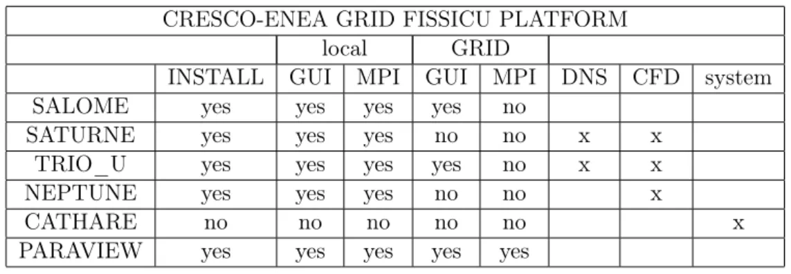
Table 1: Implementation status on CRESCO-ENEA GRID FISSICU platform This document reports the status of the FISSICU (FISsione/SICUrezza) software platform for the study of the thermal-hydraulic behavior of nuclear reactors. The idea reflects the new European policy to develop a common European tools which has lead to fund the NURISP platform project. ENEA is a user group member of the project and under a direct agreement has obtained the use of several codes. The University of Bologna participates in the effort to use and install these computational tools and other in-house developed codes on the CRESCO-ENEA GRID cluster located in Portici (near Naples). The FISSICU platform has been constructed not only to collect a series of codes that has been extensively used in this field but also to harmonize them with reference input and output formats. The aim of the platform is to solve complex problems using file exchange between different codes and large multiprocessor architecture. In this way one hopes to investigate multi-physics and multi-scale problems arising in the study of nuclear reactor components. Reference mesh and output formats are considered and conversion tools are developed. The data visualization is performed with a unique application.

In Chapter 1 we give an overview of the organization of the platform. The pur-pose of solving multi-physics and multilevel problems is discussed together with the CRESCO-ENEA GRID. The reference mesh and output formats are introduced and the visualization open-source application PARAVIEW is described.

In Chapter2 the SALOME platform is introduced along with its implementation on CRESCO-ENEA GRID. A brief explanation of the main modules KERNEL, GUI and MESH is given. The SALOME mesh generator and the file transfer service are discussed. The mesh generator is open-source but the main mesh format is the MED format which is not very popular so that conversion tools are necessary. A tutorial of the MESH module is presented.

Chapter 3 is a brief introduction to the SATURNE code. SATURNE code is an open-source code implemented on CRESCO-ENEA GRID for use in three-dimensional direct numerical simulations. The graphical user interface is introduced together with

CONTENTS

Chapter 4 is devoted to the presentation of TRIO_U and its implementation over the CRESCO-ENEA GRID. The generation of mesh and data format files is discussed together with a brief tutorial for the 2D cylindrical obstacle test. The code TRIO_U has capabilities at microscale and intermediate scale.

Finally in Chapter5NEPTUNE is described with its implementation over the CRESCO-ENEA GRID. NEPTUNE is a code that can be used in two-phase flow simulations at the intermediate scale.

FISSICU platform organization

1.1

Multiphysics and Multilevel platform

1.1.1 Multiphysics analysis

The aim of the platform is to analyze complex nuclear systems that require the coupling of different equations for different components. At present nuclear reactor thermal-hydraulics consists of different physical models (heat transfer, two-phase flow, chemical poisoning) that cannot be analyzed all at the same time. Improvements are necessary both for the physical models (heat transfer coefficient at the interface between liquid and vapor, instabilities of the interface, diffusion coefficients) and mostly for the numerical schemes (accuracy, CPU time). In the absence of direct numerical simulations the im-provement of CFD codes that rely on correlations must be based on experiments that offer sufficient resolution in space and time compared to the CFD computations. In many cases physical models lack of satisfactory experimental results and therefore numerical calculations cannot be accurate. In Figure1.1we show an example of the multi-physics approach where the physics of a nuclear core is coupled with the thermal-hydraulics of the steam generator and the pressurizer. In the upper plenum we can use a model that solves the Navier-Stokes equations while for the external loop we adopt a correlation approach. The two approaches require the use of different codes and the coupling at the interface between the two domains.

Even when experimental correlations are available for a single equation the com-plexity of the problems does not allow a whole-system simulation and even a greater computational power would be necessary to take into account the couplings. However, each physical model requires a number of parameters that are determined by the other state variables and the coupling between the equations is necessary to achieve an accu-rate and satisfactory result. For all these reasons it is important to develop tools that can manage different codes specific for a single application and perform easily a weak

FISSICU platform organization

Figure 1.1: An example of multi-physics approach for nuclear reactor (NURISP) where different equation models can be coupled to analyze a complex system.

the applications or external conversion tools are required. In the internal weak coupling all the equations are solved in a segregated way using memory to exchange data between codes. A popular format for this purpose is the MED format. The strong coupling re-quires a larger computational power but can solve all the equations at the same time giving a more accurate result.

The platform should perform these tasks automatically together with runtime schedul-ing of the programs. Another important feature of the platform is the ability to manipu-late and create input and output files with compatible formats. The SALOME software platform has been selected for these purposes and implemented on the ENEA-GRID cluster along with a selection of codes devoted to nuclear reactor thermal-hydraulics and safety analysis. Some key features of the SALOME platform are the following:

• interoperability between CAD modeling (input files) and computational software; • integration of new components into heterogeneous systems;

• multi-physics weak coupling between computation software; • a generic user friendly and efficient user interface;

• access to all functionalities via the integrated Python console.

Figure 1.2: An example of multilevel approach for a nuclear reactor (NURISP).

1.1.2 Multilevel analysis

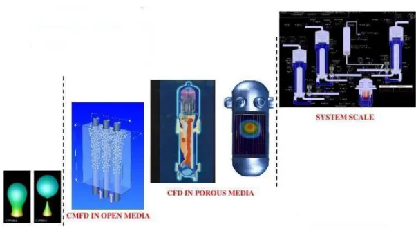
Another aspect of the complexity of nuclear reactor simulations is the different geomet-rical scales. As shown in Figure 1.2we need to investigate problems with characteristic dimensions ranging from millimeters (bubbles) to several meters (nuclear plant loop). It is not possible to solve such a complex problem in a single simulation. Therefore we model different scales with different equations that take into account the relevant physics for the selected geometry. We can roughly subdivide the phenomena into three main groups.

• Micro-scale, where direct numerical simulations (DNS) are required. Usually the Navier-Stokes system and energy equation are directly implemented without ap-proximations. The results obtained are very accurate but can only take into account small parts of the system and a limited number of processes.

• Meso-scale, where the Navier-Stokes equations can no longer be used directly. The introduction of correlations and modelings is required in order to analyze systems where thousands of microscale phenomena occur.

• Macro-scale, where the system is analyzed in its overall complexity. In this case heavy approximations must be assumed in order to simulate the whole system in a reasonable amount of time.

The phenomena in the DNS group can be simulated with commercial and open-source codes. For example ANSYS-FLUENT, CFX and Comsol multiphysics are viable

commer-FISSICU platform organization

DNS code focused on nuclear applications is TRIO_U, released only under closed agree-ment with CEA, that allows to perform simulations in three-dimensional domains. The high resolution and reliability of these codes lead to high accuracy and reproducibility of the results.

The meso-scale codes rely on correlations and averaged equations. Typical examples are turbulence models and two-phase thermal exchange. Turbulence models are widely available even for DNS codes while other correlations are specific of the applications. A nuclear engineering code of this type is NEPTUNE which is released only under closed agreement with EDF.

The system codes are very specific to the application field. In order to simulate all the system they need heavy simplifications such as the use of a mono-dimensional fluid equation. In the nuclear field we recall CATHARE (released by CEA) and the series of RELAP codes.

The CRESCO-ENEA FISSICU platform implements the following software:

• DNS: TRIO_U, SATURNE, FLUENT (already available from CRESCO), OPEN-FOAM (already available from CRESCO)

• Meso-scale: NEPTUNE, ELSY-CFD • system level: CATHARE (coming soon)

along with SALOME which performs the input/output managing and code coupling.

1.2

CRESCO-ENEA GRID

1.2.1 CRESCO infrastructure

CRESCO (Centro Computazionale di RicErca sui Sistemi Complessi, Computational Research Center for Complex Systems) is an ENEA Project, co-funded by the Italian Ministry of Education, University and Research (MIUR). The CRESCO project is located in the Portici ENEA Center near Naples and consists of a High Performance Computing infrastructure mainly devoted to the study of Complex Systems [1]. The CRESCO project is built around the HPC platform through the creation of a number of scientific thematic laboratories:

a) the Computing Science Laboratory, hosting activities on hardware and software design, GRID technology, which will also integrate the HPC platform management;

b) the Computational Systems Biology Laboratory, hosting the activities in the Life Science domain;

c) the Complex Networks Systems Laboratory, hosting activities on complex technological infrastructures.

1.2.2 CRESCO access

There are four ways to access ENEA-GRID:

a) SSH client, with a terminal interface which can directly access to one of the front-end 11

ACCESS ACCESS

Cluster Node Name SSH from SSH OS

name enea domains from world

Bologna graphlab03.bologna.enea.it yes no IRIX

pace.bologna.enea.it yes yes AIX

Brindisi campus03.brindisi.enea.it yes no LINUX

ercules.brindisi.enea.it yes yes AIX

graphbri.brindisi.enea.it yes no IRIX

Casaccia feronix0.casaccia.enea.it yes no LINUX

laran.casaccia.enea.it yes yes LINUX

prometeo.casaccia.enea.it yes yes LINUX

turan.casaccia.enea.it yes yes LINUX

Frascati bw305-1.frascati.enea.it yes no LINUX

eurofel00.frascati.enea.it yes no LINUX

lin4p.frascati.enea.it yes yes LINUX

onyx2ced.frascati.enea.it yes no IRIX

sp5-1.frascati.enea.it yes no AIX

Portici campus3.portici.enea.it yes no LINUX

graphpor.portici.enea.it yes no IRIX

Portici cresco1-f1.portici.enea.it yes yes LINUX

CRESCO cresco1-f2.portici.enea.it yes no LINUX

cresco1-f3.portici.enea.it yes no LINUX

cresco2-f1.portici.enea.it yes no LINUX

cresco2-f2.portici.enea.it yes no LINUX

cresco2-f3.portici.enea.it yes no LINUX

cresco1-fg1.portici.enea.it yes no LINUX

cresco1-fg2.portici.enea.it yes no LINUX

cresco1-fg3.portici.enea.it yes no LINUX

cresco1-fg4.portici.enea.it yes no LINUX

cresco-fpga6.portici.enea.it yes no LINUX

Trisaia campus03.trisaia.enea.it yes no LINUX

cluapple.trisaia.enea.it not yet not yet MacOSX

graphtri.trisaia.enea.it yes no IRIX

triafs.trisaia.enea.it yes yes Solaris

FISSICU platform organization

machines;

b) Citrix client, that can be installed on windows machines to access ENEA servers, including a terminal window to ENEA-GRID (INFOGRID);

c) FARO (Fast Access to Remote Objects) ENEA-GRID, that is a Java web interface available for all operating systems;

d) NX client.

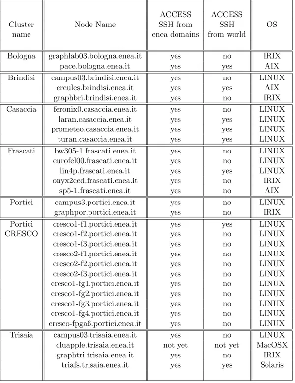
The access is limited to authorized users that are provided with ENEA-GRID user-name and password to be used on every machine of the grid. Table 1.1 shows a list of available nodes. There are a number of front-end nodes to access the platform from the external world. The main ones are:

a) sp5-1.frascati.enea.it b) lin4p.frascati.enea.it c) cresco1-f1.portici.enea.it

In this report we consider the access to a front-end node with a ssh client from a linux terminal

$ ssh -X username@cresco1-f1.portici.enea.it

If one uses the web interface FARO (http://www.cresco.enea.it/nx.html), from any

operating system, an xterm can be launched with a dedicated button. Further details on the login procedure can be found on the CRESCO website (http://www.cresco.enea. it/helpdesk.php).

1.2.3 CRESCO-ENEA FISSICU Platform

The FISSICU project is located in the directory /afs/enea.it/project/fissicu

Inside the main directory fissicu (which stands as an abbreviation for nuclear fission safety), we find the three sub-directories

- data, where the simulation results should be stored; - html, where the web pages are located

(http://www.afs.enea.it/project/fissicu/); - soft, where all the codes are installed.

At present, the following codes are available: - SALOME (see Chapter 2, executable: salome); - SATURNE (see Chapter 3, executable: saturne); - NEPTUNE (see Chapter5, executable: neptune);

- TRIO_U (see Chapter 4, executable: triou);

- FEM-UNIBO (the finite element Navier-Stokes solver developed at DIENCA - Uni-versity of Bologna).

For each code, a script (executable_env) is also available which simply sets the proper environment variables to execute the code. This procedure can be used to run the code directly without any graphical interface on a single node where the user is logged. This is also the first step for production runs which use the batch queue to run the code in parallel.

Any executable is a script in the directory /afs/enea.it/project/fissicu/soft/bin. This directory should be added to the user environment variable PATH. With the bash shell, the command line is

$ export PATH=/afs/enea.it/project/fissicu/soft/bin:$PATH This command line can also be added to the configuration file .bashrc.

1.2.4 Submission to CRESCO queues

CRESCO supports the LSF (Load Sharing Facility) job scheduler, which is a suite of several components to manage a large cluster of computers with different architectures and operating systems. The basic commands are

$ lshosts

It displays configuration information about the available hosts, as in the following output example

HOST_NAME type model cpuf ncpus maxmem maxswp server RESOURCES hostD SUNSOL SunSparc 6.0 1 64M 112M Yes (solaris cserver)

hostB ALPHA DEC3000 10.0 1 94M 168M Yes (alpha cserver)

hostM RS6K IBM350 7.0 1 64M 124M Yes (cserver aix)

hostC SGI6 R10K 14.0 16 1024M 1896M Yes (irix cserver)

hostA HPPA HP715 6.0 1 98M 200M Yes (hpux fserver)

$ lsload

It displays the current load information

HOST_NAME status r15s r1m r15m ut pg ls it tmp swp mem

hostD ok 0.1 0.0 0.1 2% 0.0 5 3 81M 82M 45M

hostC ok 0.7 1.2 0.5 50% 1.1 11 0 322M 337M 252M

hostM ok 0.8 2.2 1.4 60% 15.4 0 136 62M 57M 45M

hostA busy *5.2 3.6 2.6 99% *34.4 4 0 70M 34M 18M

FISSICU platform organization

It displays information about the hosts such as their status, the number of running jobs, etc.

HOST_NAME STATUS JL/U MAX NJOBS RUN SSUSP USUSP RSV

hostA ok - 2 1 1 0 0 0 hostB ok - 3 2 1 0 0 1 hostC ok - 32 10 9 0 1 0 hostD ok - 32 10 9 0 1 0 hostM unavail - 3 3 1 1 1 0 $ bqueues

It lists the available LSF batch queues and their scheduling and control status

QUEUE_NAME PRIO NICE STATUS MAX JL/U JL/P NJOBS PEND RUN SUSP

owners 49 10 Open:Active - - - 1 0 1 0 priority 43 10 Open:Active 10 - - 8 5 3 0 night 40 10 Open:Inactive - - - 44 44 0 0 short 35 20 Open:Active 20 - 2 4 0 4 0 license 33 10 Open:Active 40 - - 1 1 0 0 normal 30 20 Open:Active - 2 - 0 0 0 0 idle 20 20 Open:Active - 2 1 2 0 0 2 $ bsub < job.lsf

It submits a job to a queue. The script job.lsf contains job submission options as well as command lines to be executed. A typical script is

#!/bin/bash #BSUB -J JOBNAME #BSUB -q quename #BSUB -n nproc

#BSUB -oo stdout_file #BSUB -eo errout_file #BSUB -i input_file triou_env

Trio_U datafile.data

where the options to BSUB specify respectively the name of the job, the name of the queue, the number of processors, the file names for the standard and error output, the input file. The last two lines set the environment variables for the code TrioU and launch the executable with a parameter file, without the graphical interface that clearly cannot be used when submitting a job with a batch queue.

$ bjobs

It reports the status of LSF batch jobs of the user.

JOBID USER STAT QUEUE FROM_HOST EXEC_HOST JOB_NAME SUBMIT_TIME 3926 user1 RUN priority hostF hostC verilog Oct 22 13:51

605 user1 SSUSP idle hostQ hostC Test4 Oct 17 18:07

1480 user1 PEND priority hostD generator Oct 19 18:13

7678 user1 PEND priority hostD verilog Oct 28 13:08

7679 user1 PEND priority hostA coreHunter Oct 28 13:12

7680 user1 PEND priority hostB myjob Oct 28 13:17

$ bkill JOBID

It kills the job with number JOBID. This number can be retrieved with the command bjobs.

1.3

FISSICU platform input/output formats

Each software supports a large number of input and output formats that are not always fully compatible. The aim of the platform is to uniform all the codes to use the same format for input, in particular for the mesh, and for output files. Regarding the input format we select the MED and the XDMF formats. They rely on the HDF5 library that is responsible for the data storage in vector and matrix form. The MED and XDMF are driver files that access to the information stored by the HDF5 files. Regarding the output viewer we choose PARAVIEW because it is open source and can manage a large number of output formats.

1.3.1 Input mesh format

HDF5 format

Hierarchical Data Format, commonly abbreviated HDF5, is the name of a set of file formats and libraries designed to store and organize large amounts of numerical data [9]. The HDF format is available under a BSD license for general use and is supported by many commercial and non-commercial software platforms, including Java, Matlab, IDL, and Python. The freely available HDF distribution consists of the library, command-line utilities, test source, Java interface, and the Java-based HDF Viewer (HDFView). Further details are available at http://www.hdfgroup.org. This format supports a

variety of datatypes, and is designed to give flexibility and efficiency to the input/output operations in the case of large data. HDF5 is portable from one operating system to another and allows forward compatibility. In fact old versions of HDF5 are compatible with newer versions.

The great advantage of the HDF format is that it is self-describing, allowing an appli-cation to interpret the structure and contents of a file without any outside information. There are structures designed to hold vector and matrix data. One HDF file can hold a

FISSICU platform organization

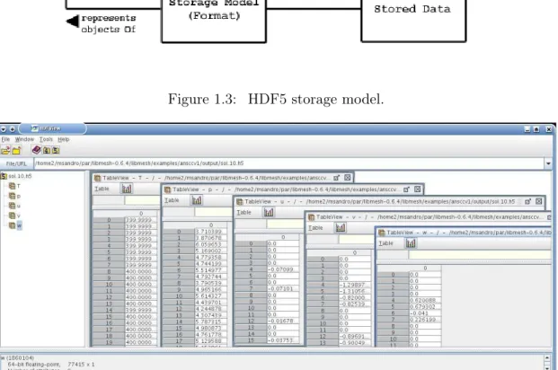
Figure 1.3: HDF5 storage model.

Figure 1.4: HDFVIEW opens HDF5 files.

The HDF5 has a very general model which is designed to conceptually cover many spe-cific data models. Many different kinds of data can be mapped to HDF5 objects, and therefore stored and retrieved using HDF5. The key structures are:

• File, a contiguous string of bytes in a computer store (memory, disk, etc.). • Group, a collection of objects.

• Dataset, a multidimensional array of Data Elements, with Attributes and other metadata.

• Datatype, a description of a specific class of data element, including its storage layout as a pattern of bits.

• Dataspace, a description of the dimensions of a multidimensional array.

• Attribute, a named data value associated with a group, dataset, or named datatype • Property list, a collection of parameters controlling options in the library.

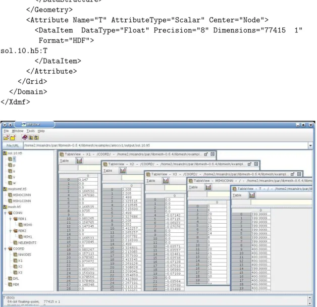
The HDF5 project provides also a visualization tool, HDFVIEW, to access raw HDF5 data. This program can be run from terminal with

$ hdfview

and a screenshot is given in Figure1.4. The panel on the left shows the list of available datasets while on the right we can see the content of each of them.

XDMF format

XDMF (eXtensible Data Model and Format) is a library providing a standard way to access data produced by HPC codes. The information is subdivided into Light data, that are embedded directly in the XDMF file, and Heavy data that are stored in an external file. Light data are stored using XML, Heavy data are typically stored using HDF5. A Python interface exists for manipulating both Light and Heavy data. ParaView, VisIt and EnSight visualization tools are able to read XDMF [8].

A brief example of a typical XDMF driver file is <?xml version="1.0" ?>

<!DOCTYPE Xdmf SYSTEM "../config/Xdmf.dtd" [<!ENTITY HeavyData ""> ]> <Xdmf>

<Domain>

<Grid Name="Mesh"> <Time Value ="0.1" />

<Topology Type="Hexahedron" Dimensions="71400">

<DataStructure DataType="Int" Dimensions="71400 8" Format="HDF"> meshxmf.h5:/MSH0CONN

</DataStructure> </Topology>

<Geometry Type="X_Y_Z">

<DataStructure DataType="Float" Precision="8" Dimensions="77415 1" Format="HDF">

../data_in/mesh.h5:/COORD/X1 </DataStructure>

FISSICU platform organization

Format="HDF">

../data_in/mesh.h5:/COORD/X2 </DataStructure>

<DataStructure DataType="Float" Precision="8" Dimensions="77415 1" Format="HDF">

../data_in/mesh.h5:/COORD/X3 </DataStructure> </Geometry>

<Attribute Name="T" AttributeType="Scalar" Center="Node">

<DataItem DataType="Float" Precision="8" Dimensions="77415 1" Format="HDF"> sol.10.h5:T </DataItem> </Attribute> </Grid> </Domain> </Xdmf>

Figure 1.5: XDMF format stores heavy data in HDF5 files.

In this example all data are stored in external files (meshxmf.h5, mesh.h5 and sol.10.h5), as shown in Figure 1.5. The data structures used in this example are Domain, Grid, Topology, Geometry and Attribute.

The organization of XDMF begins with the Xdmf element. Any element can have a Nameor a Reference attribute. A Domain can have one or more Grid elements. Each Grid must contain a Topology, a Geometry, and zero or more Attribute elements. Topology specifies the connectivity of the grid while Geometry specifies the location of the grid nodes. Attribute elements are used to specify values such as scalars and vectors that are located at the node, edge, face, cell center, or grid center. A brief description of the keywords follows. DataItem. All the data for connectivity, geometry and attributes are stored in DataItem elements. A DataItem provides the actual values (for Light data) or the physical storage position (for Heavy data). There are six different types of DataItem :

- Uniform, that is a single array of values (default).

- Collection, that is a one dimensional array of DataItems. - Tree, that is a hierarchical structure of DataItems.

- HyperSlab, that contains two data items. The first one selects which data must be selected from the second DataItem;

- Coordinates, that contains two DataItems. The first contains the topology of the second DataItem.

- Function, that is used to calculate an expression that combines different DataItems. Grid. The data model portion of XDMF begins with the Grid element. A Grid is a container for information related to 2D and 3D points, structured or unstructured connectivity, and assigned values. The Grid element has a GridType attribute that can assume the values:

- Uniform (a homogeneous single grid (i.e. a pile of triangles));

- Collection (an array of Uniform grids all with the same Attributes); - Tree (a hierarchical group);

- SubSet (a portion of another Grid).

Geometry. The Geometry element describes the XYZ coordinates of the mesh. Possible organizations are:

- XYZ (interlaced locations, an X,Y, and Z for each point); - XY (Z is set to 0.0);

- X_Y_Z (X,Y, and Z are separate arrays); - VXVYVZ (Three arrays, one for each axis);

- ORIGIN_DXDYDZ ( Six values : Ox,Oy,Oz + Dx,Dy,Dz). The default Geometry configurations is XYZ.

Topology. The Topology element describes the general organization of the data. This is the part of the computational grid that is invariant under rotation, translation, and scaling. For structured grids, the connectivity is implicit. For unstructured grids, if the connectivity differs from the standard, an Order may be specified. Currently, the following Topology cell types are defined: Polyvertex ( a group of unconnected points), Polyline(a group of line segments), Polygon, Triangle, Quadrilateral, Tetrahedron, Pyramid, Wedge, Hexahedron, Edge_3 (Quadratic line with 3 nodes), Tri_6, Quad_8, Tet_10, Pyramid_13, Wedge_15, Hex_20.

FISSICU platform organization

Attribute. The Attribute element defines values associated with the mesh. Currently the supported types of values are : Scalar, Vector, Tensor, Tensor6, Matrix. These values can be centered on : Node, Edge, Face, Cell, Grid. A summary of all XDMF structures and keywords is given in Table1.2.

MED format

Figure 1.6: MED storage format.

The MED (Modèle d’Echange de Données) data exchange model is the format used in the SALOME platform for communicating data between different components. It ma-nipulates objects that describe the meshes underlying scientific computations and the value fields lying on these meshes. This data exchange can be achieved either through files using the MED-file formalism or directly through memory with the MED Memory (MEDMEM) library. The MED libraries are organized in multiple layers:

- The MED file layer : C and Fortran API to implement mesh and field persistency. - The MED Memory level: C++ API to create and manipulate mesh and field objects in memory.

- Python API generated using SWIG which wraps the complete C++ API of the MED 21

Attribute (XdmfAttribute)

Name (no default)

AttributeType Scalar, Vector, Tensor, Tensor6, Matrix, GlobalID

Center Node, Cell, Grid, Face, Edge

DataItem (XdmfDataItem)

Name (no default)

ItemType Uniform, Collection, tree, HyperSlab, coordinates | Function

Dimensions (no default) in KJI Order

NumberType Float, Int, UInt, Char, UChar

Precision 1, 4, 8

Format XML, HDF

Domain (XdmfDomain)

Name (no default)

Geometry (XdmfGeometry)

GeometryType XYZ, XY, X_Y_Z, VxVyVz, Origin_DxDyDz Grid (XdmfGrid)

Name (no default)

GridType Uniform, Collection, Tree, Subset CollectionType Spatial, Temporal (if GridType="Collection")

Section DataItem, All ( if GridType="Subset") Topology (XdmfTopology)

Name (no default)

TopologyType Polyvertex, Polyline, Polygon, Triangle, Quadrilateral,Tetrahedron, Pyramid,Wedge,

Edge_3, Triangle_6, Quadrilateral_8, Tetrahedron_10, Wedge_15, Hexahedron_20,

Hexahedron, Pyramid_13, Mixed, 2DSMesh, 2DRectMesh, 2DCoRectMesh,

3DSMesh, 3DRectMesh

NodesPerElement (no default)

NumberOfElement (no default)

OR

Dimensions (no default)

Order each cell type has its own default

BaseOffset 0, #

Time

TimeType Single, HyperSlab, List, Range

Value (no default, Only valid for TimeType="Single") Table 1.2: XML Element (Xdmf ClassName) and Default XML Attributes

FISSICU platform organization

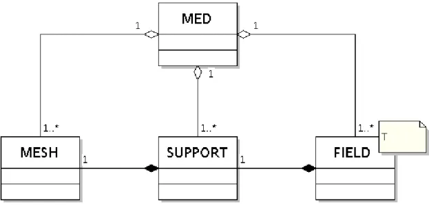
Figure 1.7: MEDMEM memory storage format. Memory.

- CORBA API to simplify distributed computation inside SALOME (Server Side). - MED Client classes to simplify and optimize interaction of distant objects within the local solver.

Two codes running on different machines can thus exchange meshes and fields. These meshes and fields can easily be read/written in a MED file format, enabling access to the whole SALOME suite of tools (CAD, meshing, visualization, other components) [4]. With MED Memory any component can access a mesh or field object generated by another application. Though the MEDMEM library can recompute a descending connectivity from a nodal connectivity, MEDMEM drivers can only read MED files con-taining the nodal connectivities of the entities. In MEDMEM, constituent entities are stored as MED_FACE or MED_EDGE, whereas in MED File they should be stored as MED_MAILLE.

The field notion in MED File and MEDMEM is quite different. In MEDMEM a field is of course defined by its name, but also by its iteration number and its order number. In MED File a field is only flagged by its name. For instance, a temperature at times t = 0.0 s, t = 1.0 s, t = 2.0 s will be considered as a single field in MED File terminology, while it will be considered as three distinct fields in the MED Memory sense.

MEDMEM supports data exchange in following formats:

- GIBI, for reading and writing the mesh and the fields in ASCII format. - VTK, for writing the mesh and the fields in ASCII and binary formats.

- EnSight, for reading and writing the mesh and the fields in ASCII and binary formats. - PORFLOW, for reading the mesh in ASCII format.

Classes. At a basic usage level, the MEDMEM library consists of few classes which are

located in the MEDMEM C++ namespace: - MED the global container;

- MESH the class containing 2D or 3D mesh objects;

- SUPPORT the class containing mainly a list of mesh elements;

- FIELD the class template containing a list of values lying on a particular support. The MEDMEM classes are sufficient for most of the component integrations in the SALOME platform. The use of the MED Memory libraries may make the code coupling easier in the SALOME framework. With these classes, it is possible to:

- read/write meshes and fields from MED-files;

- create fields containing scalar or vectorial values on a list of elements of the mesh; - communicate these fields between different components;

- read/write such fields.

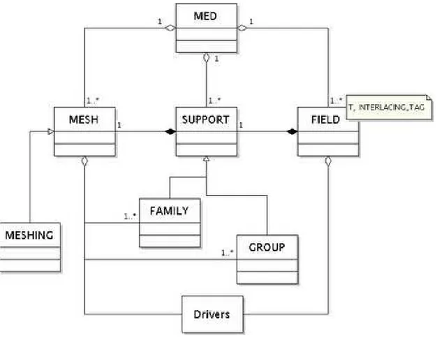
Advanced classes. A more advanced usage of the MED Memory is possible through other classes. Figure1.6 gives a complete view of the MED Memory API. It includes: - GROUP, a class inherited from the SUPPORT class used to create supports linked to mesh groups. It stores a restricted list of elements used to set boundary conditions and initial values.

- FAMILY which is used to manipulate a certain kind of support which does not intersect each other.

- MESHING which builds meshes from scratch, it can be used to transform meshes from a specific format to the MED format or to integrate a mesher within the SALOME platform.

- GRID which enables the user to manipulate specific functions for structured grids. Note that in Figure 1.6 as well as in Figure 1.7 the MED container controls all the objects it contains: its destructor destroys all the objects inside. On the other hand, the MESH, SUPPORT and FIELD objects are independent. Destroying a SUPPORT (resp. a FIELD) will have no effect on the MESH (resp. SUPPORT) which refers to it. But the user has to maintain the link: a MESH aggregates a SUPPORT which aggregates a FIELD. If the user has to delete MED Memory objects, the FIELD has to be deleted first, then the SUPPORT and finally the MESH.

MEDMEM Lists. A few enums (C enumerations) are defined in the MEDMEM names-pace :

• an enum which describes the way node coordinates or field values are stored: - MED_FULL_INTERLACE for arrays such that x1, y1, z1, . . . , xn, yn, zn;

- MED_NO_INTERLACE for arrays such that x1, . . . , xn, y1, . . . , yn, z1, . . . , zn;

- MED_UNDEFINED_INTERLACE, the undefined interlacing mode,

FISSICU platform organization

- MED_DESCENDING for descending connectivity.

The user has to be aware of the fact that the MED Memory considers only meshes defined by their nodal connectivity. Nevertheless, the user may, after loading a file in memory, ask to the mesh object to calculate the descending connectivity. • an enum which contains the different mesh entities, medEntityMesh, the entries of

which being: MED_CELL, MED_FACE, MED_EDGE, MED_NODE, MED_ALL_ENTITIES. the mesh entity MED_FACE is only for 3D and the In 3D (resp. 2D), only mesh entities MED_NODE, MED_CELL and MED_FACE (resp. MED_EDGE) are considered. In 1D, only mesh entities MED_NODE and MED_CELL are taken into account.

• The medGeometryElement enum which defines geometric types. The available types are linear and quadratic elements: MED_NONE, MED_POINT1, MED_SEG2, MED_SEG3, MED_TRIA3, MED_QUAD4, MED_TRIA6, MED_QUAD8, MED_TETRA4, MED_PYRA5, MED_PENTA6, MED_HEXA8,MED_TETRA10, MED_PYRA13, MED_PENTA15, MED_HEXA20, MED_POLYGON, MED_POLYHEDRA, MED_ALL_ELEMENTS.

1.3.2 Platform visualization

PARAVIEW on CRESCO-ENEA GRID

Inside the platform there are many applications for visualization. In order to uniform the output and the visualization we use only the PARAVIEW software. The reasons for this choice are:

• it is open-source, scalable and multi-platform;

• it supports distributed computation models to process large data sets; • it has an open, flexible and intuitive user interface;

• it has an extensible, modular architecture based on open standards.

For all these reasons the output files must be saved in a PARAVIEW readable format. From the practical point of view this is not a limitation since PARAVIEW reads a large number of formats. The following is an incomplete list of currently available readers: - ParaView Data (.pvd)

- VTK (.vtp, .vtu, .vti, .vts, .vtr, .vtm, .vtmb,.vtmg, .vthd, .vthb, .pvtu, .pvti, .pvts, .pvtr, .vtk)

- Exodus

- XDMF and hdf5 (.xmf, .xdmf) - LS-DYNA

- EnSight (.case, .sos) - netCDF (.ncdf, .nc) - PLOT3D

- Stereo Lithography (.stl)

- Meta Image (.mhd, .mha) - SESAME Tables

- Fluent Case Files (.cas) - OpenFOAM Files (.foam) - PNG, TIFF, Raw Image Files - Comma Separated Values (.csv) - Tecplot ASCII (.tec, .tp)

In ENEA-CRESCO cluster, PARAVIEW can run in two different ways: a) from console;

b) as a remote application through FARO. From console the command is :

$ paraview-3.8.0

to run the latest version of PARAVIEW (3.8.0). The other versions are available by changing the version number in the command after the − sign. We remark that PAR-AVIEW can be launched only from machines with graphical capability (with a letter g in the name). For example PARAVIEW can run from cresco1-fg1.portici.enea.it.

As a remote application one must login from the FARO web page (see Section1.2.2) and then select the PARAVIEW button. If the program runs in this mode the rendering is pre-processed on the remote machine, which guarantees a higher speed.

The PARAVIEW application

PARAVIEW is an open-source, multi-platform application designed to visualize data sets of large size. It is built on an extensible architecture and runs on distributed and shared memory parallel as well as single processor systems. PARAVIEW uses the Visualization Toolkit (VTK) as the data processing and rendering engine and has a user interface written using the Qt cross-platform application framework. The Visualization Toolkit (VTK) provides the basic visualization and rendering algorithms. VTK incorporates sev-eral other libraries to provide basic functionalities such as rendering, parallel processing, file I/O and parallel rendering [7].

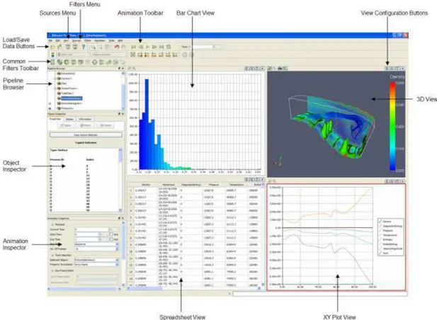
A brief explanation of the PARAVIEW GUI is given in Figure 1.8. The GUI has many panels that control the visualization. The two main panels are the View Area and the Pipeline Browser panel. The data are loaded in the View Area which displays visual representations of the data in 3D View, XY Plot View, Bar Chart View or Spreadsheet View. The visualization on the View Area is managed by the Pipeline Browser panel. The Open and Save data buttons perform the loading and saving operations for all the supported file formats. The Object Inspector panel contains controls and information about the reader, source, or filter selected in the Pipeline Browser. The most important menu is the Filters menu that is used to manipulate the data. For example one can draw the isolines of any dataset using the Contour filter. The Sources menu is used to create

FISSICU platform organization

Figure 1.8: Basic interface for PARAVIEW

new geometrical objects while the Animation toolbar navigates through the different time steps of the simulation [6].

Documentation

More information is available on the ParaView web site:

http://www.paraview.org

A wiki is also available at

http://www.paraview.org/Wiki/ParaView

and a tutorial

http://public.kitware.com/Wiki/The_ParaView_Tutorial

A list of all sources and filters can be found at

http://www.paraview.org/New/help.html

SALOME

2.1.2 Location on CRESCO-ENEA GRID

CRESCO-ENEA GRID:

executable: salome

install directory: /afs/enea.it/project/fissicu/soft/SALOME

2.1.3 SALOME overview

SALOME is a free and open-source software that provides a generic platform for nu-merical simulations. The SALOME application is based on an open and modular ar-chitecture that is released under the GNU Lesser General Public License. The source code and executables in binary form may be downloaded from its official website at

http://www.salome-platform.org. There are several version available, such as

De-bian, Mandriva and a universal package with all dependencies inside. All versions have a 32 and 64 bit version. The source code is also available to any programmer who wishes to develop and make it available for other operative system. On the CRESCO-ENEA GRID the Mandriva version (for 64 bits) is installed.

SALOME, which is also developed under the project NURISP, is a base software for integration of custom modules and developing of the custom CAD applications. The main modules are:

a) KERNEL: distributed components management, study management, general services; b) GUI: graphical user interface

c) GEOM: CAD models creation, editing, import/export

d) MESH: standard meshing algorithm with support for any external mesher (plugin-system)

e) MED: MED data files management

f) POST: dedicated post-processor to analyze the results of solver computations (scalar, vectorial)

g) YACS: computational schema manager for multi-solver coupling and supervision mod-ule.

In the FISSICU project SALOME is mainly used as mesh generator but it has many other features: interoperability between CAD modeling and computational software, integration of new components into heterogeneous systems, multi-physics weak coupling between computational software. The platform may integrate different additional codes on which perform code coupling. At the moment the integration among codes is far to be completed but some basic functionality can be used. In the platform the ideas of weak, internal weak and strong coupling are implemented. The weak coupling is performed with the exchange of output and input files. In the internal weak coupling all the equations are solved in a segregated way using memory to exchange data between codes. A popular format for this purpose is the MED library and its MEDMEM API classes. Among the various available SALOME modules, there are some samples that can be used by

the developers to learn how to create and integrate custom modules in the SALOME platform. SATURNE has a module that links to the SALOME platform, but only a beta version is available. The integration module is in development at EDF. NEPTUNE and CATHARE codes are also developing an integration module for the SALOME platform [4,5].

2.2

SALOME on CRESCO-ENEA GRID

The SALOME platform is located on CRESCO-ENEA GRID in the directory /afs/enea.it/project/fissicu/soft/Salome

The salome platform can be run in two ways: a) from console

b) from FARO website

From console one must first set the access to the bin directory /afs/enea.it/project/fissicu/soft/bin

by executing the script $ source pathbin.sh

Remark. The script pathbin.sh must be in the home directory. One must copy the template script pathbin.sh from the directory

/afs/enea.it/project/fissicu/soft/bin

and then execute the script to add the bin directory to the PATH. If the pathbin.sh script is not available one must enter the bin directory to run the program.

Once the bin directory is on your own PATH all the programs of the platform can be launched. The command needed to start the SALOME application is

$ salome

Remark. The script salome consists of two commands: the environment setting and the start command. The environment script sets the environment of shell. The start command is a simple command that launches the runSalome command.

From FARO web application it is possible to access the SALOME platform with re-mote accelerated graphics. Once FARO has been started (see Section 1.2.2) one must open an xterm. In the xterm console one must follow the same procedure as before. First, set the access to the bin directory

SALOME

by executing the script $ source pathbin.sh

SALOME starts with the command $ salome

Remark. When exiting the SALOME application we are left in a python shell. To exit press CTRL+D.

2.3

SALOME platform modules

2.3.1 Introduction

SALOME platform has seven components:

• KERNEL, that provides component management, study management and general services

• GUI, that provides a graphical user interface

• GEO, that provides a geometry module to create, edit, import/export CAD models • MESH, that provides a CAD model with standard meshing algorithms

• MED, that provides the data files management

• POST-PRO, that provides a post-processor dedicated viewer to analyze the results of solver computations

• YACS, that provides a computational schema involving multi-solver coupling

2.3.2 KERNEL

The KERNEL components is the key component of the SALOME platform. The KER-NEL module provides communication among distributed components, servers and clients: dynamic loading of a distributed component, execution of a component and data ex-change between components. CORBA interfaces are defined via IDL files and are avail-able for users in Python. CORBA interfaces for some services are encapsulated in C++ classes providing a simple interface. Python SWIG interface is also generated from C++, to ensure a consistent behavior between C++ modules and Python modules or user scripts.

2.4

SALOME file transfer service

This section introduces the SALOME file feature (Salome_file) which can be used to transfer files from one computer to another. This can be used from one program to retrieve the output file from another application and use it as input file.

2.4.1 File transfer service inside a program

Salome_fileis a CORBA object which may manage different files. First a Salome_file must be created. It is a container with no files. Files may be added to the Salome_file using the Salome_file_i interface. A file is represented by a name and a path. There are two different types of files that can be added to the Salome_file:

- Local file: the file added exists or it will be created by the user with the path and the name used in its registration.

- Distributed file: the file added exists into a distributed localization.

In order to get a distributed file, the Salome_file has to be connected with an another Salome_filethat has this file.

In the following we show a simple Salome_file with the objective to create two Salome_files: one with a local file and the other with a distributed file. Then, these Salome_filesare connected to enable the copy of the real file between the two files. #include "Salome_file_i.hxx"

int main (int argc, char * argv[]){ Salome_file_i myfile; Salome_file_i filedist; myfile.setLocalFile("localdir"); filedist.connectDistributedFile("distrdir", myfile); filedist.setDistributedSourceFile("distrdir", "localdir"); filedist.recvFiles(); };

The include Salome_file_i.hxx is necessary to use the functions and the class. In the first two lines two Salome_files are created with the command Salome_file_i. The file names are myfile and filedist. The function setLocalFile sets the path localdir of the local myfile file. The function setDistributedFile sets the path distrdir of the distributed file with name filedist. The directories must exist. Now the files are defined by name and path. The connect command connects the distributed filedist file with the local myfile file. The transfer starts with the command recvFiles.

2.4.2 Python file transfer service

The file transfer can also be obtained by using python commands. If the remote hostname is computername and we would like to copy myfile from the remote to a local computer the following python program can be used

SALOME import salome salome.salome_init() import LifeCycleCORBA remotefile="myfile" aFileTransfer= \ LifeCycleCORBA.SALOME_FileTransferCORBA(’computername’,remotefile) localFile=aFileTransfer.getLocalFile()

2.4.3 Batch file transfer service

A third way to have a service access is through the SALOME batch service. The inter-ested reader can consult the SALOME documentation.

2.5

SALOME Mesh creation

2.5.1 Import and export of mesh files in SALOME

At the moment the SALOME platform on CRESCO-ENEA GRID is not used to dis-tribute files and the implementation of coupled codes is not fully operational. The most important use of the SALOME platform is the mesh generation. SALOME offers a good open source application able to generate meshes for other applications as SATURNE and many others. For this reason it is important to use the MED format or convert such a format in more popular formats. The mesh functionality of SALOME is performed by the MESH module. In the SMESH module there is a functionality allowing importation and exportation of meshes from MED, UNV (I-DEAS 10), DAT (Nastran) and STL for-mat files. These forfor-mats are not very popular and local converters may be necessary. Mesh import. In order to import a mesh inside the SMESH module from other formats these steps must be followed:

- From the File menu choose the Import item, from its sub-menu select the corresponding format (MED, UNV and DAT) of the file containing your mesh.

- In the standard Search File dialog box select the desired file. It is possible to select multiple files.

- Click the OK button.

Mesh export. Once the mesh is generated by the SALOME MESH module the proce-dure to export a mesh is the following

- Select the object you wish to export.

- From the File menu choose the Export item and from its sub-menu select one of the available formats (MED, UNV, DAT and STL).

- In the standard Search File select a location for the exported file and enter its name. - Click the OK button.

2.5.2 Mesh tutorial from SALOME documentation Help for mesh creation can be found at

http://www.salome-platform.org/user-section/salome-tutorials

In this web page there are ten exercises from EDF:

EDF Exercise 1: Primitives, partition and meshing example. Geometric Primitives, tetrahedral and hexahedral 3D meshing, Partitions.

EDF Exercise 2: 2D Modeling and Meshing Example. Geometrical Primitives, triangular 2D mesh, Zone Refinement, mesh modification, sewing.

EDF Exercise 3: Complex Geometry meshed with hexahedra, quality controls. 3D Ge-ometry, Partition, Hexahedral mesh, mesh display, quality controls.

EDF Exercise 4: Extrusion along Path and meshing example. The purpose is to produce a prismatic meshing on a curved geometry.

EDF Exercise 5: Geometry by blocks, shape healing. Creation of a geometric object by Blocks, Primitive, Boolean Operation, Shape healing.

EDF Exercise 6: Complex Geometry, hexahedral mesh. 3D Geometry, Partition, Hexa-hedral Mesh.

EDF Exercise 7: Creation of mesh without geometry. Manual creation of a mesh. EDF Exercise 8: Pattern Mapping. Creation of a Pattern mapping.

EDF Exercise 9: Joint use of TUI and GUI. Learn to use GUI dialogs with TUI com-mands to generate a pipe with different sections.

EDF Exercise 10: Work with scripts only. This exercise is to learn working with Python scripts in SALOME. The scripts allow to parameterize studies and to limit the disk space for the storage.

2.5.3 Tutorial: step by step mesh on CRESCO-ENEA GRID

In this section we introduce step by step a mesh generation on CRESCO-ENEA GRID from the MESH module of the SALOME application.

SALOME

1. Launch salome from command line.

2. The SALOME main window will appear.

3. Click the New document button.

SALOME

5. Select the Geometry module form the dropdown menu.

6. The main window will switch to an OpenCascade scene.

7. Click the Create a box button.

8. On the dialog, use quadpipe for the Name . The dimension of the box shall be 1, 1 and 5.

SALOME

9. Zoom to the just created object.

10. Right-click on the quadpipe object in the left column. Select the Create Group option.

11. We create all the boundary regions of the box in order to put boundary conditions on them. We start from the inlet region, selecting it directly in the OCC scene.

12. Clicking the Add button, the surface should appear in the list. The number of this region must be 31. Click the Apply button.

SALOME

13. Similarly we create the outlet region (number 33).

14. We split the lateral surface in 4 regions. We start from the front one and name it wall1.

15. The number of this region is 23.

SALOME

17. wall3 region is numbered 27.

18. wall2 region is numbered 3. We can now click the Apply and Close button, since this is the last region to create.

19. To check if all the regions have been created correctly, we can use the Show Only option in the right-click menu of each object.

SALOME

21. In order to show the quadpipe object, we select show in the right-click menu.

22. We zoom to the object in the VTK scene.

23. We click on the create mesh button.

24. In the appearing dialog, we select Hexahedron (i,j,k) in the Algorithm drop-down menu for the 3D tab.

SALOME

25. In the 2D tab, we select the Quadrangle (Mapping) algorithm.

26. In the 1D tab, we select the Wire discretization algorithm.

27. Clicking on the the gear icon, we can configure the selected algorithm. We choose Average length .

SALOME

29. The mesh is now ready: we can click on Apply and Close .

30. In order to calculate the mesh, we click the Compute button in the right-click menu of the mesh we have just created.

31. If everything has gone well, a summary window will appear with some details on the mesh. In particular, we have to check that there are 1D, 2D and 3D elements.

32. Now we create the sub-regions that correspond to the boundary surfaces. We select Create groups from geometry from the right-click menu of the mesh.

SALOME

33. We select the inlet region in the left column and and click Apply .

34. We create all the six regions in the same way, selecting the mesh and the geometry element and clicking Apply until we reach the last one (wall4).

35. We recompute the mesh by clicking again Compute in order to update the mesh.

36. We can now save the SALOME study by clicking the Save button. we can name the file quadpipe.hdf.

SALOME

37. In SATURNE we need the mesh file in MED format. We can generate it via the File -> Export -> MED menu. The mesh must be selected to perform this action.

38. We name the file quadpipe.med.

This is a very simple but significative example of mesh generation, since it covers all the required steps to generate a mesh with all the features needed touse it in SATURNE or NEPTUNE. For more complete examples one can follow the tutorial suggested in Sections2.5.2. This mesh can be converted into a more popular format or used directly in many applications as, for examples, SATURNE or TRIO_U.

3.1.2 Location on CRESCO-ENEA GRID CRESCO-ENEA GRID:

executable: saturne

install directory: /afs/enea.it/project/fissicu/soft/Saturne

3.1.3 SATURNE overview

SATURNE is a general purpose CFD free software. Developed since 1997 at EDF R&D, SATURNE is now distributed under the GNU GPL license. It is based on a collocated Finite Volume approach that accepts meshes with any type of cell. The code works with tetrahedral, hexahedral, prismatic, pyramidal and polyhedral finite volumes and any type of grid structures such as unstructured, block structured, hybrid, conforming or with hanging node geometries.

Its basic capabilities enable the handling of either incompressible or compressible flows with or without heat transfer and turbulence. Many turbulence model are implemented such as mixing length, κ-ǫ models, κ-ω models, v2f, Reynolds stress models and Large Eddy Simulation (LES). Dedicated modules are available for additional physics such as radiative heat transfer, combustion (gas, coal and heavy fuel oil), magneto-hydro dynamics, compressible flows, two-phase flows (Euler-Lagrange approach with two-way coupling), extensions to specific applications (e.g. for atmospheric environment) [2,3].

SATURNE can be coupled to the thermal software SYRTHES for conjugate heat transfer. It can also be used jointly with structural analysis software CODE_ASTER, in particular in the SALOME platform. SYRTHES and CODE_ASTER are developed by EDF and distributed under the GNU GPL license.

3.2

SATURNE dataset and mesh files

SATURNE requires a specific structure for the configuration and input files. Each sim-ulation is denoted as case. One must therefore create a case directory and put all SATURNE simulations inside. For details on SATURNE file structure see Section3.3.2. SATURNE requires a dataset file (with extension xml) and a mesh file (with extension med) with the mesh geometry.

3.2.1 SATURNE mesh file

The mesh file must be in MED format. For MED format file one can see Section1.3.1

SATURNE

SATURNE GUI opens a window which is divided into three panels: top panel, option panel and view panel. The name of the study and the name of the dataset file with the corresponding path must be introduced in the top panel. The option panel consists of a tree menu with different sections. The sections are the following:

• Identity and paths where the path to the case is written; • Calculation environment with mesh selection;

• Thermophysical models with turbulence and thermal model options;

• Additional scalars with the definition and initialization of physical properties; • Physical properties with reference values, fluid properties, gravity and

hydro-static pressure options;

• Volume conditions with volume region definition and initialization;

• Boundary conditions with the definition of boundary regions and conditions; • Numerical parameters with time step, equation parameters and global

parame-ters;

• Calculation control with time average option, output control, volume solution control and output profiles;

• Calculation management with user arrays, memory management and start/restart options.

The mesh should be opened and checked through the section Calculation environment. In this section there are also some mesh quality tools. The mesh must be saved in MED format and constructed in such a way that the boundary zones are marked as special regions. These regions will appear in the Boundary conditions section where the bound-ary conditions must be defined. The SALOME GUI defines the boundbound-ary conditions as shown in Figure3.3. The parameters as the time step length and the number of the time steps can be set in Numerical parameters. A screenshot of the Numerical parameters is shown in Figure3.4. The computation can be started from the start/stop computation panel in the Calculation management section. This panel appears in Figure 3.5where the number of processors can be set. For more details one can see the example in Sec-tion3.4or the documentation of the SATURNE code. The SATURNE GUI generates a dataset file like the following:

<?xml version="1.0" encoding="utf-8"?>

<Code_Saturne_GUI case="cyl" study="case" version="2.0"> <solution_domain>

... <meshes_list>

<mesh format="med" name="cyl1.med" num="1"/> 61

</meshes_list> ...

</solution_domain> <thermophysical_models> <velocity_pressure>

<variable label="Pressure" name="pressure"> <reference_pressure>101325</reference_pressure> </variable> ... </thermophysical_models> <numerical_parameters> <multigrid status="on"/> <gradient_transposed status="on"/> <velocity_pressure_coupling status="off"/> <pressure_relaxation>1</pressure_relaxation> <wall_pressure_extrapolation>0</wall_pressure_extrapolation> <gradient_reconstruction choice="0"/> </numerical_parameters> <physical_properties> <fluid_properties>

<property choice="constant" label="Density" name="density"> <initial_value>1</initial_value> <listing_printing status="off"/> <postprocessing_recording status="off"/> </property> ... </fluid_properties> ... </physical_properties> <boundary_conditions> <variable/>

<boundary label="BC_1" name="1" nature="inlet">inlet</boundary> ... </boundary_conditions> <analysis_control> <output> <postprocessing_mesh_options choice="0"/> ... </output> <time_parameters> <time_step_ref>0.01</time_step_ref> <iterations>100</iterations> <time_passing>0</time_passing>

SATURNE <zero_time_step status="off"/> </time_parameters> <time_averages/> <profiles/> </analysis_control> <calcul_management> ... </calcul_management> <lagrangian model="off"/> </Code_Saturne_GUI>

This file can also be modified without the GUI by editing a template dataset XML file. The file is subdivided into various sections such as Calculation environment,

Thermophysical models, Additional scalars, Boundary conditions, Numerical parameters and Calculation management. Inside each section we can see the corresponding options.

3.3

SATURNE on CRESCO-ENEA GRID

3.3.1 Graphical interface

The SATURNE code is located on CRESCO-ENEA GRID in the directory /afs/enea.it/project/fissicu/soft/Saturne

Once the PATH is set for the directory /afs/enea.it/project/fissicu/soft/bin by executing the script

$ source pathbin.sh

as it is explained in Section1.2.3, the SATURNE GUI starts with the command $ saturne

Remark. Not all libraries are yet available at the moment for the CRESCO architecture. We suggest to run SATURNE GUI on a personal workstation.

The GUI is used to set up the simulation creating a data.xml file. The solution of the case must be run in command line mode or in batch mode as explained in the next section.

3.3.2 Data structure

SATURNE requires a specific structure for the configuration and input files. Each simula-tion is denoted as case. We can therefore create a cases directory and put all SATURNE simulation files inside.

Inside this directory, each case will have its own directory (for example case1, case2) and there must be a MESH directory, where all the meshes are stored.

cases +-- case1 +-- case2 ...

+-- MESH

Inside each case directory, we have to create the four sub-directories - DATA, where the xml configuration file is stored;

- RESU, that is used for the outputs;

- SCRIPTS, that hosts the execution scripts;

- SRC, in which we can put some additional source file.

During the execution, SATURNE will generate some temporary files that are by default stored in the tmp_Saturne directory in the user home directory. This directory must be periodically cleaned by hand, as there is no automatic procedure.

3.3.3 Command line execution

In order to execute the application in a shell we must first set up the environment using the script

saturne_env

that is located in the directory

/afs/enea.it/project/fissicu/soft/bin

Remark. The saturne_env script consists of the following lines #! /bin/bash

export cspath= \

/afs/enea.it/project/fissicu/soft/Saturne/2.0rc1/cs-2.0-beta2/bin export CSMPI=$cspath/../../openmpi-1.4.1/bin

export PATH=$cspath:$PATH

In order to run a case one must first create a directory and put the following files in it:

• data.xml that is the configuration file of the case • mesh.med that is the mesh file (in MED format) There are two ways to run the code:

a) from console

b) using the runcase script