Optimization algorithms for signal synchronization and bus priority on urban arteries

(1)

Roma Tre University

Ph.D. in Computer Science and Engineering

Optimization Algorithms for Signal

Synchronization and Bus Priority on

Urban Arteries

(2)

(3)

Optimization Algorithms for Signal Synchronization and Bus Priority on Urban Arteries

A thesis presented by Andrea Gemma

in partial fulfillment of the requirements for the degree of Doctor of Philosophy

in Computer Science and Engineering Roma Tre University

Dept. of Informatics and Automation December 2010

(4)

Tutor:

Prof. Dario Pacciarelli Reviewers:

Prof. Michael Florian Prof. Gaetano Fusco

(5)

(6)

(7)

vii

Abstract

This thesis is aimed at defining a simulation model representing the vehicular flow along an urban road artery with traffic signals. This platoon-based model can simulate the behavior of private and public transport vehicles and gives the opportunity to implement priority strategies for the latter. As a result of the simulation, it is possible to calculate the vehicles delay caused by the presence of traffic lights and this information was used to define a fitness function representing the quality of traffic light synchronization.

In the second part of the work two optimization algorithms have been realized to minimize the fitness function: A genetic algorithm and particle swarm algorithm. The two algorithms, known to have comparable performance, were compared on real instances of some main roads in the urban area of Rome.

(8)

viii

Acknowledgements

I am very grateful to all the people who have directly or indirectly contributed to the birth of this Ph.D. thesis. Special thanks to my tutor Prof. Dario Pacciarelli, to Prof. Gaetano Fusco of “La Sapienza” University of Rome, to Prof. Cipriani of the Department of Civil Engineering of Roma Tre University of Rome and to my colleagues and friends. I would also like to thank the members of AuTORI Automation and Industrial Management Laboratory of Roma Tre University. At last, I would like to thank Ing. Valentina Conti for her support throughout the PhD.

(9)

(10)

x

List of Figures

Figure 2-1 - Update schema for signal plan ... 28

Figure 2-2 - Vehicle trajectory without traffic light priority ... 36

Figure 2-3 - Bus Trajectory with green extension priority ... 39

Figure 2-4 - Bus Trajectory with green anticipation priority ... 40

Figure 2-5 - Bus Trajectory with green insertion priority ... 40

Figure 2-6 - Resolution algorithm structure of the dynamic traffic

assignment model ... 48

Figure 2-7 - Dynamic equilibrium assignation algorithm in dynameq 50

Figure 2-8 - Triangular flow-density diagram ... 51

Figure 2-9 - Simplified model of queued vehicle ... 52

Figure 2-10 - Spatial discretization of the network arcs ... 55

Figure 2-11 - v-k relation (Greenshield's equation changed) ... 56

Figure 2-12 - Equation of state of the Cell Transmission Model ... 62

Figure 2-13 - Representations of convergence and divergence ... 64

Figure 2-14 - Node delay for a fore-delayed platoon (case A). ... 67

Figure 2-15 - Node delay for a rear-delayed platoon (case B). ... 68

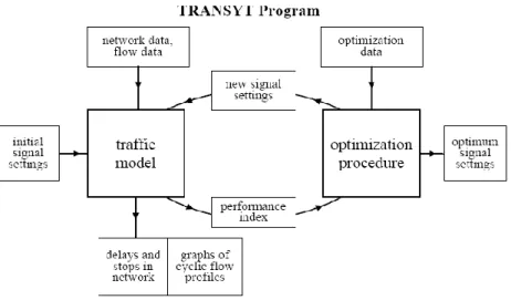
Figure 2-16 - IT architecture of the TRANSYT resolution model and

procedure (Source: Vincent, Mitchell, Robertson. User guide to

Transyt Version 8, 1980) ... 72

Figure 2-17 - Transyt arc delay model (source: Dion et al., 2004) ... 78

Figure 2-18 - Spillback queue and impossibility for the upstream

vehicles to exploit the green (from synchro 6 manual) ... 81

Figure 2-19 - Reduction in capacity effect due to queues (from synchro

6 manual) ... 81

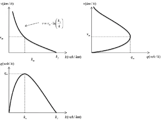
Figure 3-1 - Greenberg law ... 102

Figure 3-2 - Greenshield linear model ... 104

Figure 3-3 - Greenberg logarithmic model ... 105

Figure 3-4 - Delay of a vehicular platoons at a sincronized artery node

... 108

(13)

xiii

Figure 3-5 - Representation of the progression of a platoon ... 109

Figure 3-6 - Example of platoon of type A ... 112

Figure 3-7 - Example of platoon of type B ... 113

Figure 3-8 - Example of platoon of type C ... 114

Figure 3-9 - Wave front ... 116

Figure 3-10 - Representation of kinematic wave in the flow-density

diagram ... 117

Figure 3-11 - Stop wave ... 118

Figure 3-12 - Start wave ... 119

Figure 3-13 - Delay model flow chart ... 121

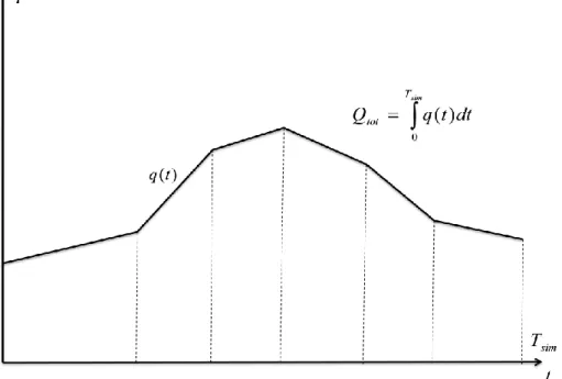
Figure 3-14 - Example of demand curve ... 124

Figure 3-15 - Recombination of platoons ... 125

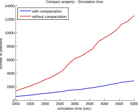
Figure 3-16 - Number of platoons required for a simulation applying or

not applying the compaction property with the cange of the

simulation time ... 127

Figure 3-17 - Cycles order ... 128

Figure 3-18 - Catch-UP ... 130

Figure 3-19 - Example of spillback phenomenon ... 131

Figure 3-20 - Spillback in the space-time diagram... 131

Figure 3-21 - Example of reclassification in case of spillback ... 133

Figure 3-22 - Spillback condition (a). Push-back method (b).

Reclassification method (c). ... 134

Figure 3-23 - Spillback condition ... 136

Figure 3-24 - Push-back method ... 137

Figure 3-26 - Trajectories of vehicles in different platoons in case of

oversaturation ... 138

Figure 3-27 - Extended delay model flow chart ... 139

Figure 3-28 - Green advance ... 145

Figure 3-29 - Green extension ... 146

Figure 3-30 - Conflict in the assignment of the priority ... 148

(14)

xiv

Figure 3-32 - Relations between models and data ... 151

Figure 3-33 - Example of the progression of platoons generated by the

model (buses are highlighted in black) ... 151

Figure 4-1 - Scanning of six different dimensions of the objective

function ... 154

Figure 4-2 - Scanning of the objective function between two generic

configuration of three road artery. Alpha is the coefficient of

convex combination between the configuration. ... 155

Figure 4-3 – Comparison between trend of algorithm with random

initial population or with intelligent construction of initial solution

... 160

Figure 4-4 - Matrix rappresentation of Genome ... 161

Figure 4-5 - Crossover of type 1 ... 163

Figure 4-6 - Crossover of type 2 ... 164

Figure 4-7 - Crossover of type 3 ... 165

Figure 4-8 - Trend of the algorithm with the three crossover methods

... 166

Figure 4-9 - Trend of the algorithm with different crossover rate... 167

Figure 4-10 - Simulation for different mutation rate ... 169

Figure 4-11 - Simulation for different interval.Δ=[pmin

mut

, pmax

mut

] 170

Figure 4-12 - Simulation for different interval.Δ=[pmin

mut

, pmax

mut

] in

Colombaroni, Gemma and Fusco (2009) ... 170

Figure 4-13 - Simulation for different elite rate ... 172

Figure 4-14 - Trend of the objective function for the genetic algorithm

with best parameters ... 173

Figure 4-15 - Comparison between trend of algorithm with random

initial population or with intelligent construction of initial solution

... 176

Figure 4-16 - Agent movement relative to two sizes in the space of

research ... 177

(15)

xv

Figure 4-18 - Trend of the algorithm with different speed parameters

... 180

Figure 4-19 - Trend of the algorithm with different best local

parameters ... 180

Figure 4-20 - Trend of the algorithm with different best global

parameters ... 181

Figure 4-21 - Trend of the algorithm with different random parameters

... 181

Figure 4-22 - Trend of particle swarm algorithm for different values of

inertia parameter ... 182

Figure 4-23 - Trend of the objective function for the particle swarm

algorithm with best parameters ... 183

Figure 4-24 - Application of Hill-Climbing after 300 iterations or with

premature stop at 50 iterations ... 185

Figure 4-25 - Comparision between PSO and GA ... 186

Figure 4-26 - Average Fitness ... 187

Figure 4-27 - Execution time ... 189

Figure 5-1 - Average unitary delays at nodes on the whole artery for 3

demand levels (high, average, low) ... 191

Figure 5-2 - Total vehicles served in simulation for the 3 demand levels

(high, average, low) ... 192

Figure 5-3 Average unitary delay at each node for the high demand

scenario ... 193

(16)

16

1 Introduction

In an urban network, a point where more delay accumulates is at the intersections. The cause of this delay is the sharing of the intersections by the different traffic flow: the same road space used for traffic movements must be shared, alternating, between two or more current vehicular conflicts. The average capacity of the intersection is therefore less than half the capacity of the road. Especially with very high traffic flows, the intersection becomes a bottleneck due to the progression of vehicles that are delayed. In order to better manage the sharing of the intersection, it will be necessary to use the traffic lights. When along a road artery there are most signalized intersections, coordination between the different traffic lights becomes crucial: the interruption of progression due to the alternating cycles of the traffic signal makes the flow not constant, therefore, to the generic approach, there will be time intervals characterized by a large number of incoming vehicles and other intervals with a more modest flow or even zero. Hence it is possible to organize the traffic lights in such a way that red time interval overlaps, as far as possible, with the interval of low flow, properly synchronizing the beginning of the green in such a manner that interval of green starts when the intense traffic flow arrives. Ideally, one would expect that no vehicle is stopped and then the delay may be canceled. This condition is essentially impossible to fulfill but in most real cases an appropriate offset of the green of traffic lights can reduce travelling times significantly. Although it is not possible to allow all vehicles to progress along the route without stops at the nodes, in other respects, it is possible to reduce the waiting time or the number of vehicles stopped along the artery. In the case of one-way streets, the

(17)

17

problem is complicated by the presence of incoming / outgoing vehicles that make sure that in the artery there is not a single compact platoon. As for two-way streets, the problem is further complicated by the requirement to take into account each node in both directions. The offset of a generic node, in fact, affects not only the delay at that node, changing the sequence of the vehicles from that node, but also the delay in all downstream nodes, and thus, in the two-way street, the offset of a generic node affects the delay in all nodes of the artery. Within the scope of the synchronization problem, then, the average delay of the artery is a scalar function of vector of offset (or stages) of all nodes. The independence of the effects of the various nodes, which could be positive or negative, easily shows that the synchronization problem of minimum delay is a not convex problem. For this reason it is still frequently used an another approach: usual traffic signal optimization methods seek either to maximize the green bandwidth or to minimize a general objective function that typically includes delays, number of stops, fuel consumptions and some external costs like pollutant emissions. Without loss of generality, henceforth this method well be called minimum delay problem. This method is related to physical variables that are to be minimized; anyway, it is a non-convex problem and existing solution methods do not guarantee to achieve the optimal solution. The maximal bandwidth method maximizes an opportunity of progression for drivers and does not reduce delays necessarily. Nevertheless, it is an almost concave problem and there are efficient solving algorithms to find the optimal solution. The traffic lights cause not only the delay but also allow to apply priority strategies of transit. As for private transport, the strategies attempt to reduce delay in two ways: by reducing the probability that a transit vehicle encountering a red signal, and, if this does

(18)

18

occur, by reducing the wait time until the green signal. Since the passage of the bus is more sparse, it is possible to implement the signal priority strategies temporarily only in their passage. The crucial importance of traffic lights and the need for tools to optimize the delay by the synchronization was the starting point of the research presented in this work.

1.1 Definitions

Although this work has been done in computer engineering and operations research for its full understanding requires a good knowledge of the transport sector. Where possible, to make the text as complete as possible, many aspects of transport engineering will be explained. It is not of interest in this work to explain all phenomena that are behind the flow of vehicular and so many concepts were implied assumption that the reader's knowledge. For those who need to know more about you suggest the following reference books (Cascetta, 1998) and (Sheffi, 1985)

Below, to give uniformity to the reading of this work will be a short description of the main variables used in the traffic light synchronization and in particular in this work. Each of these parameters will be given a uniform meaning and representation in later chapters:

Ci [sec]: Cycle time for the generic traffic light intersection i. Traffic light

cycle is defined as any complete sequence of switch on (and off) of traffic lights at the end of which returns the same configuration of the lights existing at the beginning of the sequence. When will speak of synchronization between multiple traffic lights will refer to this size without linking to any intersection.

(19)

19

In such cases, the cycle is the common cycle at all intersections also called synchronization cycle.

q [vehicles/sec]: vehicular flow. It defines the flow of a current the average

number of vehicles passing through a section in unit time.



: offset. In the case of synchronization of plans between different traffic light intersection the offset represents the phase shift with respect to the common cycle synchronization. The offset is represented with adimensional values in the range [0 ÷ 1). Where will be appropriate, in this work, this size will defined in seconds and in the range [0 ÷ C).

s [vehicles /sec]: saturation flow. The saturation flow is the maximum number

of vehicles that can cross a stop line of an intersection per unit time in the presence of continuous queue. The saturation flow depends on the geometric characteristics of the intersection, on the composition of the flow and on the control mode of traffic lights.

y: saturation degree. The saturation degree is the ratio between traffic flow

and the flow of saturation. This quantity is an indicator of the level of congestion.

gif: effective green split (in this work simply green split) is the ratio between

the effective green and the duration of the cycle of the traffic light on intersection i in phase f. For the analysis of the traffic, sometimes, is convenient to consider, instead of the real length of the green, the duration of effective green for which it is assumed that vehicles may flow to the values of saturation flow, and then with a constant time distance equal to

1 s

. The

(20)

20

introduction of the concept of effective green split can easily determine the maximum flow on the basis of saturation flow and the traffic light cycle.

g s

q 

rif: effective red split is defined as 1- gif or the part of the cycle for the phase f

is not used by the traffic flow for transit across the intersection i.

L [sec]: The traffic light cycle cannot be used to completely by the vehicles

stream to the values of saturation flow of each current. In fact there is the time lost in which the intersection is not used completely. The time lost was due mainly to three contributions:

 Transient state of vehicles in the queue at the beginning of the green phase;

 The transitory of exiting of vehicles from intersection at the end of the green phase and during the yellow phase;

 the time between the end of yellow and the beginning of green of the next phase.

The lost times at the beginning and at the end of green are used to determinate the duration of effective green.

F: Phase means that part of the plan during which a particular traffic light

signal configuration is constant.

A traffic light plan for a single intersection is defined by the duration of a cycle as well as the phase transition and duration. It can be described in two way:

(21)

21

 on the structure: by the phase, their duration and the transaction between their;

 on the time step: by start times and end times for each light for each phases in the interval [0÷C]

(22)

22

2 State of Art

Traffic signal timing is implemented either by fixed time or traffic-responsive control. In the fixed time control, signal timing plans are designed according to the prevalent traffic conditions observed through historical surveys. Traffic responsive control makes use of real-times measurements provided by automatic traffic detectors. It can be implemented in two different ways: plan-selection or plan-generation. The first method selects the most appropriate pre-calculated plan according to the traffic conditions observed in real-time. The plan-generation method applies a control logic that adjusts signal settings on-line, according to real-time traffic counts. The last method is theoretically the most effective, since it is flexible enough to carry out quick adjustments of signals to better accommodate the traffic at each junction. It has also some shortcomings, related to the difficulty of obtaining stable solutions for all possible traffic conditions as well as a higher number of traffic detectors, which implies, on one hand, a greater cost and, on the other hand, a lower robustness of the control system with respect to detector failures. For these reasons, plan-selection methods are often still applied and off-line optimization methods for traffic signal synchronization are still widely studied in order to pre-compute the optimal plans.

Traffic signal optimization on road arteries consists of two problems: the solution algorithm and the progression model used to compute the values of the objective function. In order to improve the algorithm, several authors combined in a different way two synchronization approaches: the minimum delay and the maximal bandwidth.

(23)

23

Cohen (1983) used the maximal bandwidth as initial solution of the former problem; Cohen et al (1986) constrained the solution of the former problem to fulfill maximum bandwidth; Hadi et al. (1993) used the bandwidth as objective function; Malakapalli (1993) added a simple delay model to the maximal bandwidth algorithm; Gartner (1994) introduced a flow-dependent bandwidth function; Papola (2000) expressed the delay at nodes as a closed form function of the maximal bandwidth solution. Since the first platoon dispersion model introduced by Robertson (1969), progressively more complex models have been developed. Park et al. (1999) introduced a genetic algorithm-based traffic signal optimization program for oversaturated intersections consisting of two modules: a genetic algorithm optimizer and mesoscopic simulator. Dazhi et al. (2006) proposed a bi-level programming formulation and a heuristic solution approach for dynamic traffic signal optimization in networks with time dependent demand and stochastic route choice. Chang et al (2004) proposed a dynamic method to control an oversaturated traffic signal network by utilizing a bang-bang-like model for oversaturated intersections and TRANSYT-7F for the unsaturated intersections. This work presents an optimization method consisting of a mixed genetic-hill climbing algorithm, which applies a new platoon based delay model that generalizes the analytical model developed by Papola et al (2000). In such a way, it is possible to deal even with non stationary traffic demand and non synchronized signal settings. It introduces also more general assumptions on drivers's behavior. The algorithm is rather similar to the well-established Transyt solving procedure Transyt-7F (McTrans-Center, 2006), which respect to it introduces some additional flexibility aimed at improving the algorithm efficiency.

(24)

24

In addition to private transport, in this work, the problem of minimum delay for public transport with priority strategies was tackled. Several methods exist to ensure priority to buses with respect to general traffic in urban areas. Among these, signal priority strategies attempt to reduce delay in two ways: by reducing the probability of a transit vehicle encountering a red signal, and, if this does occur, by reducing the wait time until the green signal. The objective of this study is modeling and simulating a mathematical procedure to provide bus priority along a synchronization artery, through the combination of passive and active bus priority strategies.

Passive priority is defined as the use of static signal settings to reduce delay for transit vehicles. Such strategies can be as simple as increasing the green split for the phase in which the transit vehicle has right of way. Signal coordination is another strategy that can be used to benefit transit vehicles. Arterial progression, for example, can be designed to favor transit vehicles by timing the green band at the average transit vehicle speed instead of the average automobile speed, which is typically faster (Davol, 2001). More effective coordination strategies can combine the maximum green bandwidth and minimum delay problems used in private transport and already mentioned. However, it has been observed that passive strategies have limited value in order to improve the global transport performances (Skabardonis, 2000). Active strategies address these limitations by altering signal settings dynamically and only when necessary, in order to minimize delay to an approaching transit vehicle. Several studies have been performed to apply active priority strategies: Liao et al. (2007) takes advantage of the already equipped Global Positioning System on buses to develop an adaptive signal priority strategy that could consider bus schedule adherence, number of

(25)

25

passengers, location and speed; (Stevanovic, et al., 2008) presents a genetic algorithm formulation that optimizes four basic signal timing parameters and transit priority settings using VISSIM micro simulation as the evaluation environment. A bus priority algorithm could also be integrated into an adaptive network signal control model. For example, SCOOT (McDonald, et al., 1991) system has a number of facilities that can be used to provide priority to buses or other public transport vehicles; the signal timings are optimized to benefit the buses, either by extending a current green signal (an extension) or causing succeeding stages to occur early (a recall). Priority facilities are also available in UTOPIA (Mauro, 1991) system, in which optimal strategies are determined at the higher level on the basis of area traffic prediction, while traffic light control is actuated at the local level according to traffic conditions at individual intersections. The aim of control strategies is to minimize the total time lost by private vehicles, while ensuring that public transport vehicles are not stopped at signalized intersections. The present paper introduces a traffic platoon model and a heuristic algorithm to optimize preset signal synchronization plans that can include and simulate active bus priority strategies at some signals.

2.1 Methods of control

It is used to classify the types of traffic control according to the characteristics and dimensions of the problem which involves:

 Methods of control for synchronized intersections deal directly the space-time interaction of vehicular flow;

(26)

26

 Methods of Traffic Actuated Control (also known in real time) adapting the characteristics of traffic lights to demand variability;  The fixed time control methods that assume the validity of

steady-state;

 Methods of equilibrium traffic control that look for a good network configuration compatible with the resulting change of route of users, instead, the traditional methods of traffic lights control calculate the parameters assuming constant traffic demand and the choice of route as invariants.

The methods of control for synchronized intersections can be distinguished, on the base of parameters of control, between methods of maximum green bandwidth (or "green wave") and maximum performance or can be distinguished on the base of technology used to make synchronization between several intersections, in systems with centralized architecture and distributed systems architecture.

The methods of Traffic Actuated Control can be classified into systems of selection (real-time actuation and off-line calculations) or plan-generation (on-line calculations and dynamic regulation); the latter is then divided into open circuit control systems (if the variables measured are the inputs for the models) or closed circuit (if the variables measured are the product of models of regulation). Finally, an important division concerns the possibility to discern specific vehicle categories, such as public transport and emergency vehicles, with the possibility to advantage them.

(27)

27

The steady-state traffic control can be achieved with a fixed time method, if the traffic flow remains constant for a fixed period of time at least one order of magnitude higher than the traffic light cycle, or with a plan-selection method, where the temporal variations of traffic flow occurs slowly from one period to another, so as that by measuring the value of the flow in some sections, it is possible to recognize the particular configuration of traffic and to actuate a pre-calculated plan to control the measured condition.

2.1.1 Steady-State of control

The steady-state control is used, therefore, to optimize the traffic light parameters for particular time interval, assuming that in each interval flows are known and constant. In the fixed time control the flows are calculated on statistic information. In the plan-selection control, instead, the flows are detected real-time with traffic sensor; on the bases of this measures, the control system sets the most appropriate plan, applying predefined plan. From the methodological point of view, both the flows models and resolving procedure are similar for the two control methods. In both cases, the flow is considered constant in the time of application of the plan and therefore it is possible to apply models of progression or loading of the network in steady-state flow. It is possible to define, for each intersection, a traffic light cycle, which represents the time period in which, within the range of stationary, the same configurations of traffic light are repeated. In both cases, moreover, it is possible to define a policy control based on knowledge of the average of each flows of traffic and, in the case of synchronized intersections, on the progression of vehicles on the network.

(28)

28 Update

An important aspect of fixed time control or plan-selection is a periodic update of traffic lights plans. The adjustment is needed to adapt the control to the changes in long-term demand and in traffic flows on the network, dependent on seasonal or structural variations. Figure 2-1.

Figure 2-1 - Update schema for signal plan

The plan-selection method requires a monitoring system to classify the traffic pattern and a recognizing system to find the best match between the pattern and the pre-calculated plans.

(29)

29

2.1.2 Dynamic control

Principles of the dynamic traffic flow control

Dynamic control strategies are designed to adapt in the short term the signals configuration to the variability of the traffic flow at intersections. These strategies are potentially more efficient but, in turn, much more expensive from the operational costs point of view, since they require the installation, implementation and maintenance of control systems in real time (measurements, transmission of information, a central controller, and local controllers).

Dynamic control strategies use instantaneous measurements carried out by detectors (generally, inductive), placed in proximity of the intersection at the beginning or at the end of each approach. Through appropriate algorithms they set the green time, the offset and the cycle time for the plan in question on the basis of the traffic flow detected.

The time horizon of each planning is estimated for a medium-long period H (e.g. 60s), but the results are actually applied only for a much shorter period of time (e.g. 4s). Then, new information are collected and a new optimization issue is solved by planning an time horizon H as much long. This way the process is prevented from adopting myopic strategies based only on the optimization of the present situation.

One of the most spread algorithms for this kind of strategies is SCOOT (Hunt, et al., 1981). Recently, new multiple traffic-adaptive methods have been proposed: OPAC (Gartner, 1982), PRODYN (Farges, et al., 1983), CRONOS

(30)

30

(Boillot, et al., 1992), COP (Sen, et al., 1996), RHODES (Mirchandani, et al., 2001), UTOPIA (Mauro, et al., 1989).

Binary variables in the formulation of the problem are the main issue of these strategies, because they require the employment of algorithms with exponential complexity for a global minimization. Practically, some algorithms resolve the problem with the complete enumeration of the solution (brute force), whereas others adopt a dynamic programming. Since the resolution of these algorithms is extremely complex, the control strategies, theoretically adaptable to the whole network, can be applied in real time to an only one intersection. That leads to the realization of the system by employing several excellent decentralized strategies (at each road junction), whose choices are heuristically coordinated by a high-level control. An exception is CRONOS, which uses a global heuristic optimization method with polynomial complexity, enabling to take into consideration simultaneously multiple intersections and obtaining this way a local but not global minimum.

"Store and forward" approach

A particular category of the traffic-adaptive strategies is represented by the approaches based on the "store-and-forward" philosophy. This type of network formation was suggested for the first time by (Gazis, et al., 1963) and by then it has been used in many worthy works.

The main idea of the store-and-forward model is the introduction of a simplification providing the mathematical description of the traffic flow without recurring to binary variables. It is crucially important because it allows to use many highly efficient polynomial-complex methods of control

(31)

31

and optimization (linear, quadratic, nonlinear programming and multivariable regulators). On the other hand, it permits real time coordinated control also on networks on a large scale.

The fundamental simplification is introduced when modelling the outflow qi

of an arc i. The outflow qi in the discrete time k derives from:

 

i i i

s

C

k

g

k

q



Eq. 2-1

where gi(k) represents the green duration for the arc i and si is the

corresponding saturation flow. If the discrete time interval is equivalent to the cycle time C, then qi will be equivalent to the average flow during the

corresponding cycle, instead of being formed as equivalent to si during the

green phase and null during the red one. In other words, each network arc is assumed to get a constant and uninterrupted outflow (until the demand keeps to be sufficient). As a consequence of this simplification:

 time discretization cannot be lower than the cycle time C, so decisions in real time could not be made more than once per cycle;  the oscillation of the platoon on the arcs, due to the alternation

between the green and red phases, are not described by the model;  the effect of the offset for the consecutive intersections cannot be

represented by the model.

In spite of the restrictions, the appropriate use of the "store-and-forward" model can bring to efficient coordinated control strategies for networks on a

(32)

32

large scale, as demonstrated by several studies of simulation. A recent application of this strategy is originated by the TUC algorithm (Diakaki, et al., 2001) based exactly on a formulation of this kind.

2.2 Priority measures for buses

A wide range of methods were developed in order to let the public means get priority on the general traffic in urban areas. Some of them are:

 virtual or physical vehicle flow split systems;  traffic light priority systems.

The fact of considering buses separately from the general traffic already provides the strongest kind of bus priority. Some of these systems include:

 Bus-only streets: roads where entrance is denied to all vehicle but the ones with priority (not only means of public transportation but also emergency vehicles);

 Busways: fully detached ways for buses travelling on one or both directions, usually placed at the middle of the carriageway. Buses travelling on a Busway can work normally or be driven through physical or electronical tools. The Busway can be associated to a platooning management with platoons of buses and trolleybuses stopping simultaneously and providing so the same features of an underground or LRT (Light Rail Transport);

 Reserved lane: a reserved lane for buses and other vehicles having priority and travelling in the same direction, placed next to the lane for vehicles with no priority. This one can be physically detached or

(33)

33

simply signaled through road surface markings. Some countries are characterized by full-time or part-time traffic hours (rush hour and off-peak hour);

 Reverse reserved lane: a lane of the carriageway reserved for public and other means with priority; in this lane though the means with priority always travels in the opposite direction of the means with no priority travelling in the contiguous lane. This kind of reserved lane is quite always physically detached from the rest of the infrastructure and works full-time; it is often used on one-way streets in order to reduce the travelling distances of buses and to provide reserved access to areas of interest for passengers (shops, offices, etc.).

In order that these reserving tools perform completely their priority function of public transportation, in terms of travel time saving and reduction of the delay during its working, they must be integrated with the traffic regulation systems to realize a traffic light priority system.

The methods to grant priority to public means at traffic lights can be grouped into the following categories:

 Passive priority: traffic signal timing is designed to provide priority benefits to bus flows without buses being monitored one by one.  Active priority: traffic signal timing is changed to give priority at

traffic lights to each bus individually approaching intersections, on the basis of the control strategies. Active priority can be reached through:

(34)

34

o special sensors on the mixed lanes able to identify public means (by their length or weight);

o systems included in the onboard equipment (like tags or transponders) communicating with the street infrastructures at the intersections.

 Traffic light priority using pre-signals: it is a queue management method using traffic lights to manage congestion and queues, in order to put buses in a position where their travel is not delayed by queues of private vehicles. This method involves pre-signals, whose task is to keep general traffic at the upstream of the intersection, in order to assure the buses a reserved access to them.

Road space reservation Traffic light priority

Physical Virtual With sensors Without sensors Bus-only street

Busway Reserved lane Reverse reserved lane

Bus lane Active Pre-Signals

Passive

Table 1 - Diagram of reserving systems of classification

For this work active and passive traffic light priority measures were employed without using pre-signals, which can represent a possible future development.

2.2.1 Strategies of signal priority for

buses

The signal priority strategies for public transportation is aimed at reducing the delay of buses at the signalized intersections. The basis for this special consideration is the high capacity of vehicles. Typically, traffic signals are

(35)

35

designed to minimize the total delay of all the vehicles at an intersection. However, minimizing the delay of the vehicles could not be optimal considering the passenger load of the vehicles. For example, a delay of 30 seconds for a crowded bus clearly is not equivalent to a 30-second delay for a vehicle with an only one passenger. So it would be better as a unit of measurement the total delay per person instead of the total delay for vehicle. Granting priority to public means is then more suitable way to minimize the total delay per person and maximize the number of people passing. In Figure 2-2 it is shown how the delay for a means of public transportation can be caused by a traffic signal in absence of traffic light priority methods. The trajectory of a means of public transportation is drawn in a space-time diagram and the horizontal straight line represents a traffic signal with its indication displayed during the time. If in the vehicle trajectory an forbidden-way traffic light comes, the delay increases until the displaying of free-forbidden-way traffic signal when the vehicle can proceed. Signal priority strategies attempt to reduce the delay in two ways:

 by reducing the probability that a means of public transportation gets an forbidden-way traffic signal;

 by reducing the waiting time, in which the traffic signal gives again free way, when encountering an forbidden-way signal.

(36)

36

Figure 2-2 - Vehicle trajectory without traffic light priority

Passive signal priority strategies

Passive priority is defined as the use of static traffic regulation methods to reduce the delay of public transportation.

Many are the static signal priority strategies:

 Increase of the green time for the road artery with public transportation lines. It is the simplest kind of passive priority strategies and provides more green time for roads with public transportation lines through increased green split for the phase in which the public transport vehicles have the right to pass. Since it reduces the percentage of cycle time during which the phase of the public transportation receives the forbidden-way signal (reduction of red time), both the probabilities that the bus arrives during the red phase and the average waiting time decrease.

(37)

37

 Use of short traffic light cycles. Another passive strategy is to use a certain duration of the short cycle, that can reduce the delay shortening the waiting time up to the successive green phase. However, this implies a reduced capacity for the intersection, especially due to the increasing of the time lost (the time in each cycle during which there are no vehicle movements). The loss of time is typically caused by full-red time plus the starting delay at the beginning of each phase (time of evacuation at setting in move), then in each cycle it is independent of the cycle duration lost during the loss of time. If an intersection is close to saturation, delays could be currently increased. But if there is an excess of capacity, this strategy can reduce the delays for single vehicles.

 Division of the green phase across the corridors of the public transportation. With this strategy the free-way phase across the corridors of the public transportation implies a double phase within the same cycle. The duration of the cycle can remain unchanged if each of the two green phases is half of the original duration. The benefits means of transport obtained through this strategy include the reduction of the time amount between the green phases reducing the waiting time for the vehicles that received the red time.

 Traffic light synchronization. In this strategy the arterial progression, for example, can be designed to favor the public transportation vehicles through the timing of green bands with the average bus speed instead of the average private vehicles speed. Although this strategy increases the travel time for the drivers, it helps assuring that the public transportation vehicles can be in line with the traffic signal

(38)

38

progression. However, in the urban area the progression for the buses could be difficult to respect because of the stops, which impede this vehicles to move at a constant rate within the network.

A general problem occurring with the passive priority strategies is the fact that they typically lead the intersection to work overall less efficiently, especially if the frequency of the public transportation is not very high. For this reason, the strategies cannot be always realizable in particular in conditions of oversaturation. In some cases, using short cycles or longer green splits for the public transportation, the oversaturation of the intersection occurring would cause long queues and delays. They represent the limits of the passive priority strategies, but in different cases they are the only realizable options in particular when the evaluations of the costs require the use of the existing control system, so the recent research quantity within the passive strategies is minimal (Skabardonis, 2000).

Active signal priority strategies

The active strategies face the limitations of the passive strategies by alternating dynamically the traffic light regulations and, only when necessary, by making adjustments in real time and by timing traffic lights to minimize the delay of the public means to the approach. That is intensive from the infrastructural point of view with respect to the passive strategies, because it requires tools to detect the public vehicles upstream on the intersection and control systems ahead to use the strategies to accept the priority.

There are three basic actions that a control system can perform to react to the detection of the means of public transportation:

(39)

39

 Green extension in the current phase. If the bus approaches to the intersection at the end of the green time interval in its direction, then the current green time interval can be extended until the vehicle overcomes the intersection as shown in the picture below.

Figure 2-3 - Bus Trajectory with green extension priority

Without extension, the vehicle would have to wait for the green light of the successive cycle with a consequent significant delay.

If the vehicle is approaching to a red light signal, there are two options:  If the vehicle gets normally the green light in the successive phase,

the current phase could end in advance to enable the vehicle to get sooner the green light. That occurs if the vehicle arrives at the intersection almost at the end of the red phase for its direction, as shown in the picture below.

(40)

40

Figure 2-4 - Bus Trajectory with green anticipation priority

 If other phases have to be served before the return of the normal green time, a short phase can be inserted for the approach of the public means with the control system that can function normally again once the vehicle is passed. This case is shown in Figure 2-5, where the control system interrupts its normal traffic signal plan to serve the phase of public transportation before returning to the regular timing.

(41)

41

More interesting is the effect on private traffic that active priority strategies can cause.

Under conditions of light traffic flow, active priorities can have little effects on the general traffic flow, because the exceeding capacity within the cycle can be redistributed to the phase of public transportation.

However, active priority can have greater negative effects during the rush hour, when the intersections operate very close to saturation with short or no time to lose for the movements of the non-public means.

In turn, the active strategies divide into 3 categories:  Unconditional strategies;

 Conditional strategies;  Adaptive strategies.

The unconditional strategies provide the state of priority to each public means detected. This means that the control system will try to start one of the priority actions described above, once any means of public transportation is detected. The disadvantage of this strategy is the fact that priority could be granted to any public vehicle, which might not need it, as for example a vehicle in advance with respect to its schedule. However, such priority requires only information about the presence of the vehicle sent to the control system. The conditional strategies grant the state of priority on the basis of certain criteria, which in most cases are linked to the specific means of transport. The most common criterion for conditional priority is the vehicle delay with

(42)

42

respect to its schedule. However, other criteria, such as the vehicle frequency or the passenger load, are taken into consideration for different applications. The adaptive signal priority strategies for public means use control patterns based on the optimization, in order to determine if and how to grant priority. In some patterns, the delay of the public means is considered together with the delay of all the other vehicles. The control system then calculates the optimal solution consisting in the way to distribute the green time among the current approaches. As phases and times are not fixed, adaptive strategies do not require the predefinition of specific priority actions, like the extension or the insertion of a phase. The control system changes constantly the distribution of green time according to the demand. Priority strategies for public means can easily be implemented within more adaptive existing systems, giving more importance to public transportation vehicles in the optimization routine. The implementation of the traffic light priority for public means within an already existing adaptive network control system can cause some errors.

This kind of system in fact considers as part of the optimization the effects of the global regulation, while giving signal priority is competence of a local control system. That can lead to conflicts of aims in the optimization giving then sub-optimal results. Another problem is the fact that the most part of the adaptive control system use macroscopic traffic models in their routine of estimation and optimization. These models cannot catch certain details in the movements of the public transportation means. For example, the waiting time at the stops of the public transportation and the interactions among the public vehicles and the others would not be considered, so that the travel time for the public means could be underestimated. Finally, the restrictions on the

(43)

43

optimization could limit the opportunities for the priority of the public means, especially during the rush hour when it is more important. For example, a binding factor can be the maximum length of queue acceptable on each approach; in very congestioned conditions this restriction could be always active, not enabling to assign the additional green time to the approach to reserve.

The tools to detect the presence of public means, to which the active traffic light priority is granted, can be:

 ordinary sensors on the reserved lanes;

 special sensors on the mixed lanes able to detect public means (by a different Earth's magnetic field alteration);

 systems included in the onboard equipment (like tags or transponders) communicating with the street infrastructures at the intersections.

The most recent systems help managing platoons in real time with information to passengers at the bus stops, assuring the traffic signal reserving on the basis of the service needs, aiming at improving regularity and punctuality. There is a clear tendency to increase the use of GPS (Global Positioning System) technology for bus localization. This technology helps lower the operative costs and represents a flexible solution for the localization of the public means.

(44)

44 2.3 Existing simulation and optimization

models

The model proposed in this work is built both on a simulation model to evaluate the performance of a signalized road artery and on an optimization algorithm for the traffic light synchronization. This chapter presents the most known simulation and optimization models of the traffic light synchronization, available in the literature and often applied on real cases or on commercial developments. Many models proposed are in fact software and appear as black-box to the user. So the most of the information presented is taken from the manuals coming with software or available online.

2.3.1 Simulation models

Traffic simulation models are divided into:  microscopic and discrete models;

 macroscopic and continuous models (discretized to implement a simulation);

 mesoscopic models.

The traffic microsimulation models help viewing lifelike movements of the single vehicles and following the development of traffic on the road network. These models, simulating the behavior of each single vehicle with its own origin and destination, provide all the elements for a detailed quantitative analysis. They are disaggregate models, as they reproduce the movement of

(45)

45

the single vehicle, but often are also used for aggregate analysis (flows, lengths of the queue, travel times, etc.).

In the macrosimulation the traffic is normally described as a flow defined by behavioral rules based mainly on the interaction of vehicles among them and with the infrastructure. The macroscopic models, also known as continuous time and space models, are based on the continuous simulation of the traffic. The mathematical theory underlying such models is set on the time and unidimensional dynamics, respecting the flow conservation laws.

In the last few years some mixed, mesoscopic models were proposed, based on the simulation of the microscopic or quasi-microscopic kind, which presents macroscopic features (as for example the concepts of aggregate speed and density). In general, mesoscopic models have the great advantage of being less onerous from the computational point of view, but present the disadvantage of less detailed representations of the vehicles behavior.

Dynameq

DYNAMEQ, designed by M. Florian (2005), is a dynamic traffic assignment (DTA) model, which uses some variants of the gradient method and the method of successive averages (MSA) to determine the choice of path in a condition of dynamic equilibrium.

The choice of path are shaped as decisional variables ruled by the user optimal principle, according to which each user of the network aims at minimizing their costs and so the travel time on the path used. All the users access the network information and therefore to the travel time on all the paths (used and not used).

(46)

46

The resolution algorithm is an iterative procedure realized to converge towards these conditions and is characterized by two main components:

1. a method to determine a new set of path flows variable in time considering the knowledge on the travel times in the previous iteration;

2. a method to determine the arc flows and the travel times resulting from a given set of incoming path flows. That refers to the network loading phase carried out through an efficient event-traffic simulation model. The model represents explicitly the available regulation systems and catches realistically the congestion phenomena, such as the queue formation and their propagation from arc to arc (spillback).

Two different approaches are normally used to simulate the user choice behavior: a dynamic "en route" assignation and a dynamic equilibrium assignation. In DYNAMEQ the approach used is the search for an approximate solution in equilibrium conditions.

In the equilibrium assignment problem only the pre-trip path choices are taken into consideration and they are the choices made by the user before taking their path. The choice of path are shaped as decisional variables ruled by the user optimal principle, according to which each user of the network aims at minimizing their costs and so the travel time on the path used. All the users access the network information and therefore to the travel time on all the paths (used and not used). The resolution algorithm is an iterative procedure realized to converge towards these conditions.

(47)

47 The resolution algorithm

The resolution algorithm used in DYNAMEQ consists of two main components beyond the phase of calculation of the minimum dynamic paths:

1. a method to determine a new set of path flows variable in time considering the experience developed on the travel times in the previous iteration;

2. a method to determine the arc flows and the travel times resulting from a given set of incoming path flows.

Moreover, the algorithm requires an initial set of path flows. The general structure of the algorithm is shown in Figure 2-6.

(48)

48

Figure 2-6 - Resolution algorithm structure of the dynamic traffic assignment model

Defining K the set of all paths, the path flows of h_k , kK input are determined by a variation of the method of successive averages (MSA), applied to each origin/destination couple and time interval  .

An initial set of possible solutions is calculated assigning the demand for each time interval on a set of successive minimum paths. From the second iteration and up to a maximum predefined N number of iterations, the arc travel times variable in time after each loading are used to determine a new set of dynamic minimum paths added to the set of current paths.

(49)

49

In the iteration n,nN, the volume assigned on each path belonging to an initial set is equivalent to

n g_i

, where g is demand of O/D pair in the time _i

interval  _{. Afterwards, for each iteration m, m>N, the minimum paths are} identified among those actually used and the path flows are redistributed across the paths known.

If the flow on a particular path goes under a predetermined value, the path is not taken into consideration and its flow is distributed on other paths used. This heuristic approach is similar to the Lawphongpanich, and Hearn's algorithm (1984) for the solution of the stable fixed-demand equilibrium model.

(50)

50

Figure 2-7 - Dynamic equilibrium assignation algorithm in dynameq

It is important to know that although this model is very close to the macroscopic models of outflow, is indeed a discrete model. The network loading procedure, carried out through an event simulation, moves the single vehicles on the network arcs.

The network loading model

The simulation model core is the car following simplified model: ] ) ( , ) ( min[ ) (t x t V x t R L x_f  _f   _l   Eq. 2-2

(51)

51

where xf(t) is the trajectory of a vehicle (function in time), L is the actual length of the vehicle, R is the user reaction time, V is the free speed and ε is an arbitrarily short time interval. The subscripts f and l denote respectively the trajectories of the follower and the leader vehicles. This model take into consideration the only free speed (without acceleration constraints) combined with a simple model of collision avoidance and can be easily represented through the well-known triangular flow-density diagram, also called fundamental diagram of traffic flow (Mahut, 2000).

Figure 2-8 - Triangular flow-density diagram

This relation can be solved rigorously, as well as it is possible to calculate the time in which a vehicle enters and exits each arc using this formula:

                        _ _ L X R X t V L R t V X X t tn n n n X L 2 2 / 2 1 1 1 1) , (0) , ( ) ( max ) 0 ( 2 Eq. 2-3 Q 0 40 0 80 0 120 0 160 0 200 0 0 9 0 K F lo w (v e h ic le /h /la n e ) 1 6 0 3 0 -W 12 0 1 Density (vehicle/h/lane) V

(52)

52

where X1 and X2 are the lengths of the upstream and downstream arcs with

respect to the position x=0, V1 and V2 are the free speeds respectively on these

two arcs and the subscripts represent the vehicles sequentially numbered. This arc formulation provides a very practical and computational-efficient way to shape the traffic flow without calculating analytically the state variations (position, speed, etc.) of each vehicle at each instant. Please note how this expression can be applied only to the case of an arc with just one lane (Figure 2-9).

Figure 2-9 - Simplified model of queued vehicle

In case of a multi-lane road, a different formulation needs to be used to calculate the entrance and exit time for each vehicle, but also to catch the interactions among vehicles because of the lane change (Mahut, 2000). The model for multi-lane roads develops a series of heuristic procedures to form the lane choice by the user, who bears in mind their wished path upstream to their current position, the lanes likely to be used for the successive turn and the main traffic flow conditions on each lane interposed between the driver and the end of the arc.

The above said model of arc determines the instant when a vehicle wishes to enter the arc as function of the entrance and exit time history. The information is used for a rigorous application of the previous model of queued vehicle.

0 x

X

(53)

53

In short, the car following model is extended in a such a recursive way that it is applied to a sequence of vehicles. For instance, rather than forming the relation between vehicle 1 and vehicle 2 (the higher number follows the lower one) and the consequent relation between vehicle 2 and vehicle 3, the model enables to express directly the interaction between vehicle 1 and vehicle 3. That can be extended to any number of vehicles, and this is actually the essence of the arc expression previously mentioned. From a conceptual point of view, since the first cause for the delay in a network is due to the intersections, the role of dynamics in this model is to propagate appropriately the delay between upstream and downstream vehicles. That is to say that these delays can affect the entrance and exit times in the arc. Instead of forming explicitly the position of each vehicle to determine when the congestion of the arc starts to affect these entrance times, the exit delays are transmitted directly in entrance. This peculiar feature - the ability to solve rigorously the traffic flow model on the whole arc - has been proved also in the case of the kinematic wave model based on the fundamental triangular diagram (Newell, 1993).

This dynamic traffic flow model, that can be characterized as a model continuous in time and space and with discretized flow, is combined with a node model representing explicitly the predetermined traffic signal systems and also shaping the interactions among vehicles at non-signalized intersections through a gap-acceptance logic. The combined system is then solved by using an event algorithm enabling to form the whole network. Event models are basically different from the models for discrete time interval, that is:

(54)

54

 the models for discrete time intervals provide that at each time step (usually 1 second or less) all the data required for each vehicle in each single model (queued vehicle, lane change, gap-acceptance, path choice) are updated and the outputs (acceleration, deceleration, etc.) are re-calculated;

 event models provide that the single submodels are updated only if one of the inputs changes considerably. So the single submodels assure that their outputs keep their validity as long as the input data keep constant. An event is generated in a specific point if the information changes. Usually, the performance of an event results in the creation of one or many sequences of events.

The result in this case is a very computational-efficient event model, which though respects also the basic laws of the traffic flow and represents explicitly the congestion mechanism that occurs in real life.

From all that, higher calculation time savings derive with respect to the time interval simulation models (in one or two levels of size).

The computational time are particularly important in the context of dynamic traffic assignment models, which must perform several iterations to solve the equilibrium assignment. The time factor is even more important, because dynamic traffic assignment models must be applied to big networks.

(55)

55 Dynasmart

In Dynasmart (Mahmassani, et al., 1992) the traffic flow simulation derives by the MPSM model1: the generic vehicle (or the group of vehicles) travels on the network according to the discrete space intervals and its position is updated every 6 seconds (spatial and time discretization).

Figure 2-10 - Spatial discretization of the network arcs

The traffic flow model used consists in the speed-density relation deriving by the change of the well-known Greenshield's equation:

              j f k k v v v v 0 ( 0) 1 Eq. 2-4 where:  v₀: minimum speed  v_f:speed with null flow  k_j:maximum density  : calibration parameter

Dynasmart then lets vehicles move on each arc at the speed resulting from Greenshield's equation changed, knowing the density at the end of the previous time step.

1

Optimization algorithms for signal synchronization and bus priority on urban arteries