Universit`
a degli Studi di Pisa
Facolt`
a di Scienze Matematiche, Fisiche e Naturali
Corso di Laurea Magistrale in Informatica
A Framework to compare
text annotators and its
applications
October 2012
Master Degree Thesis
Candidate
Marco Cornolti
Supervisor
Prof. Paolo Ferragina
Universit`
a di Pisa
Co-Reviewer
Prof.ssa Anna Bernasconi
Universit`
a di Pisa
Contents
1 Introduction 3
2 Some topic retrieval problems 6
2.1 Terminology . . . 6
2.2 Definition of problems . . . 7
2.3 Our contribution: A hierarchy of problems . . . 10
2.4 Conclusions . . . 12
3 New evaluation metrics 13 3.1 Metrics for correctness evaluation . . . 14
3.2 Finding the mentions (for Sa2W and A2W) . . . 18
3.3 Finding the concepts (for Sa2W and A2W) . . . 18
3.4 Similarity between systems . . . 19
3.5 Conclusions . . . 22
4 The comparison framework 23 4.1 Code structure . . . 23
4.2 Running the experiments . . . 26
4.3 Extending the framework . . . 29
4.4 Conclusions . . . 39
5 Datasets, Systems and Wikipedia 40 5.1 Wikipedia and its graph . . . 40
5.2 Topic-retrieval systems . . . 41
5.3 Available datasets . . . 43
5.4 Comparing two systems for a given dataset . . . 46
5.5 Conclusions . . . 47
6 Experimental Results 49 6.1 Setting up the experiments . . . 49
6.2 Results for Experiment 1: news . . . 51
6.3 Results for Experiment 2: tweets . . . 61
6.4 Results for Experiment 3: queries . . . 62
6.5 Experiments about runtime . . . 63
7 Future Developments 67
7.1 Definition of new problems . . . 67
7.2 Chimera: mixing systems together . . . 70
7.3 Conclusions . . . 70
Appendices 72
A Formulary 73
Chapter 1
Introduction
Concerning topic-retrieval
Texts in human languages have a low logical structure and are inherently am-biguous because of this structure and the presence of polysemous terms. Never-theless, the typical approach of Information Retrieval to manage text documents has been, up to now, based on the Bag-of-words model (BoW) [38]. In this model, texts are represented as the multi-set of terms they contain, thus dis-carding any possible structure or positional relations existing among the terms. Moreover, terms are interpreted as sequence of characters and mapped to inde-pendent dimensions into a huge Euclidean space, so that synonymy and poly-semy issues are not taken into account at all. Because of its simplicity, BoW is at the core of most (if not all) current text retrieval systems; but anyone is aware of its obvious limitations.
Recently, some research groups tried to overcome these limitations by propos-ing a novel approach which consists of addpropos-ing some “contextual information” to text representation, identifying meaningful mentions in the input text and linking them to their corresponding topics provided by a proper ontology. See Figure 1.1 for an example. This process is nowadays called “text annotation” and the software systems which implement it are called “topic annotators” or “topic-retrieval systems”. These systems differ to each other by the ontology used to extract the annotated concepts (E.g. Wordnet [10], CiC [24], Wikipedia, Yago 2 [16]) and by the algorithms employed to derive these annotations.
The power of these systems resides in the underlying structure which in-terconnects the topics attached to the texts within the ontology. The most successful systems are currently the ones based on Wikipedia, and these sys-tems have been applied to improve the performance of IR tools on many classic problems such as: the categorization or the clustering of documents; the
topic-based search over a web collection, and so on.
The success in the use of Wikipedia lies in the fact that this online ency-clopedia offers free (as in freedom) and open access to a huge knowledge base that, despite not being guaranteed to be correct, provides a very high quality thanks to the process used to author Wikipedia pages [22]. Wikipedia is open to the contribute of everyone, including anonymous users, and pages authoring is collaborative. The lack of a central authority potentially leads to a low reli-ability, but since the review process is distributed as well, involuntary mistakes or malicious errors are quickly found and corrected [25].
Wikipedia is a huge mine of semi-structured information. First of all, Wiki-pedia pages can be seen as a representation of specific and unambiguous topics. Their abstract and their content give a detailed description of the topic, meta-data like the hits count and the revisions give information about the popularity of the concept and how frequently its description changes, pages are catego-rized by a rich set of categories, and anchors of links to a Wikipedia page offer
a set of commonly used synonyms for the concept the page is about. But
the most interesting information lies into the structure of its graph, where the nodes are the Wikipedia pages and the edges are the links between pages: the shape of the graph can tell much about how semantically close two pages are [31, 40, 12, 15, 34].
Many topic-retrieval systems use this direct graph, and the whole informa-tion that Wikipedia offers, to solve synonymy and polysemy issues in the input text [14, 28, 5, 8, 9]. The approaches followed by the systems differ in the way this information is exploited.
Our Contribution
These systems give surprisingly good results, but the research have followed specific and target-oriented trends, leading to disuniform terminology and ap-proaches, despite targeting the same set of problems. To address the research, it is fundamental to have a consistent framework that offers a formal base upon which it’s possible to build new theories, algorithms and systems.
Moreover, there is no improvement without measuring, and literature gives a plenty of ways to determine the performance of a system. Unfortunately, the used methods are inconsistent with each other.
The aim of this thesis is to formalize such a framework, presenting both some of the problems related to topic-retrieval and a set of measures to assess the performance of the systems in solving those problems. The result of this work is a benchmarking framework software that performs the measures on the systems.
Figure 1.1: An example of a topic retrieval task: from the un-structured text on the left, the unambiguous topics are extracted.
In Chapter 2, we discuss the formal framework, presenting the problems related to topic-retrieval. To solve the lack of uniformity in the measures, our contribution is the presentation in Chapter 3 of a set of metrics that can be used to fairly compare the topic annotators to each other. Despite sounding straight-forward, the definition of this metrics hides non-trivial issues. The implemented benchmarking software based on these metrics is presented in Chapter 4.
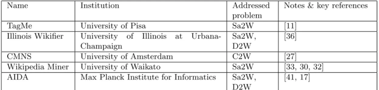
In Chapter 5 a snapshot of the state-of-the-art topic annotators is given, as well as the available datasets to perform the benchmarking. Results of the benchmark of these annotators on the dataset are given in Chapter 6 and show that some systems, like TagMe, Illinois Wikifier and Wikipedia Miner, give good results with a rather low runtime, suggesting their application to large-scale datasets.
In Chapter 7 some lines of possible future development are presented. To facilitate the reading of this thesis, all defined formulas are reported in a table in Appendix A, with a brief description.
Chapter 2
Some topic retrieval
problems
What’s in a name? that which we call a rose By any other name would smell as sweet.
– William Shakespeare, Romeo and Juliet, Act II
2.1
Terminology
As stated in the Introduction, literature about topic retrieval presents a wide variability of terminologies. The following terminology, that will be used in the next chapters of this thesis, is a compromise between the popularity of a term in literature, its clarity, and the avoidance of conflicts with other works that may lead to ambiguity.
• A concept is a Wikipedia page. It can be uniquely identified by its Page-ID (an integer value).
• A mention is the occurrence of a sequence of terms located in a text. It can be codified as a pair hp, li where p is the position of the occurrence and l is the length of the sub-string including the sequence of terms. • A score is a real value s ∈ R, s ∈ [0, 1] that can be assigned to an
annotation or a tag. Higher values of the score indicate that the annotation (or tag) is more likely to be correct.
• A tag is the linking of a natural language text to a concept and is codified as the concept c the text refers to. A tag may have a score: a scored tag is encoded as a pair hc, si, where s is the score.
This thesis Milne-Witten [33] Han-Sun-Zhao [13] Ferragina et al. [11] Ratinov et al. [36] Meij et al. [27]
concept sense entity sense Wikipedia
ti-tle
concept
mention anchor name mention spot mention
tag annotation
annotation link entity linking annotation mapping
score score ρ-score score
Table 2.1: Terminology used by some of the works in literature.
• An annotation is the linking of a mention in a natural language text to a concept. It can be codified as a pair hm, ci where m is the mention and c is the concept. An annotation may have a score: a scored annotation can be codified as hm, c, si, where s is the score.
Table 2.1 reports a “vocabulary” of the different terminology used in other publications.
2.2
Definition of problems
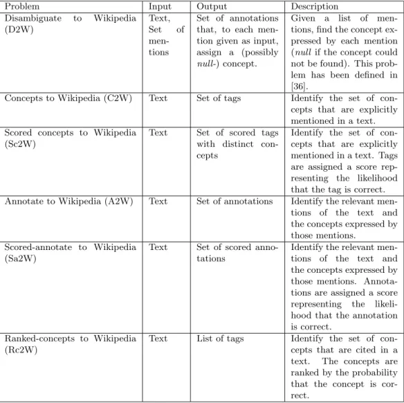
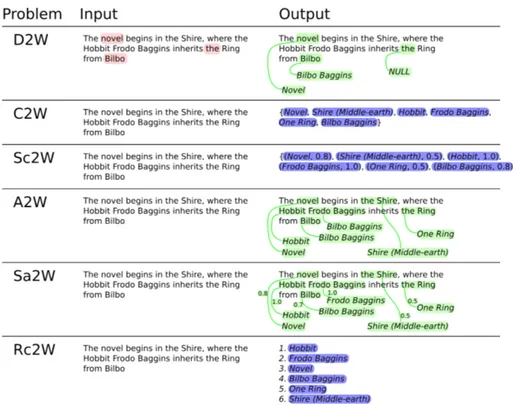
We define a set of problems related to the retrieval of concepts in natural lan-guage texts. The difference between these problems can be seen as subtle but leads to different approaches to measure the performance of a topic-retrieval system. The definition of the problems related to topic retrieval is given in Ta-ble 2.2, where each proTa-blem comes with the type of the input (that is, the type of a problem instance) and output (the type of the solution). Figure 2.1 shows some examples of input and correct output for the given problems.
2.2.1
The topic-retrieval problems and their applications
Problems presented Table 2.2 face different applications. Let’s give some shallow examples. For a document clustering based on the document topics, we are interested in finding only the tags, and not the annotations of a document, hence this application would depend on the the solution of C2W and its scored variant Sc2W. Successful applications of this problem are presented in [18, 20, 39]. Rc2W, that returns concepts ordered by the likelihood that they are correct, can as well be used. Applications such as user profiling and document retrieval are as well based on these problems.
Annotations are useful for assisting human reading. Reading a text, like an article on an on-line newspaper, the meaning of some mentions could be unclear. Annotating the text adding a link from these mentions to the right
Problem Input Output Description Disambiguate to Wikipedia (D2W) Text, Set of men-tions Set of annotations that, to each men-tion given as input, assign a (possibly null-) concept.
Given a list of
men-tions, find the concept ex-pressed by each mention (null if the concept could not be found). This prob-lem has been defined in [36].
Concepts to Wikipedia (C2W) Text Set of tags Identify the set of
con-cepts that are explicitly mentioned in a text. Scored concepts to Wikipedia
(Sc2W)
Text Set of scored tags
with distinct con-cepts
Identify the set of con-cepts that are explicitly mentioned in a text. Tags are assigned a score rep-resenting the likelihood that the tag is correct.
Annotate to Wikipedia (A2W) Text Set of annotations Identify the relevant
men-tions of the text and
the concepts expressed by those mentions.
Scored-annotate to Wikipedia (Sa2W)
Text Set of scored
anno-tations
Identify the relevant
men-tions of the text and
the concepts expressed by those mentions. Annota-tions are assigned a score
representing the
likeli-hood that the annotation is correct.
Ranked-concepts to Wikipedia (Rc2W)
Text List of tags Identify the set of
con-cepts that are cited in a
text. The concepts are
ranked by the probability that the concept is cor-rect.
Figure 2.1: Examples of instances of the topic-retrieval problems and their correct solution. Mentions are highlighted in red, (scored) tags in blue, (scored) annotations in green. Concepts are in italics.
Reduction Instance adaptation Solution adaptation
A2W ∝ Sa2W No adaptation. discard the scores, take only the concepts with a
score higher than a given threshold.
D2W ∝ A2W Take only the text,
discard the mentions.
let M be the set of mentions to disambiguate, part of the instance. Take only the annotations hm, ci of the solution such that m ∈ M . Set the concept of all other mentions in M to null.
Sc2W ∝ Sa2W No adaptation. Discard the mentions, take only the concepts and
their score. Let A = a1, · · · , an be the solution of
problem Sa2W. If two annotations ai and aj have
the same concept, discard the one with lower score.
Rc2W ∝ Sc2W No adaptation. Take only the concepts with a score higher than a
given threshold. Rank the concepts by their score, discard the scores.
C2W ∝ Rc2W No adaptation. Turn the list into a set.
C2W ∝ A2W No adaptation. Discard the mentions, take only the set of concepts.
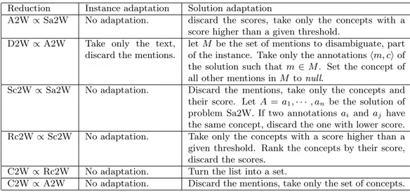
Table 2.3: Reduction between problems. A ∝ B means A can be reduced to B (hence B is harder than A).
Wikipedia concept would help a human understand the text. This is called text augmenting and lies upon the solution of A2W and its scored variant Sa2W. D2W could also be used for this application, interactively asking the human user which mentions should be annotated.
2.3
Our contribution: A hierarchy of problems
It is of key importance to note that the defined problems are strictly related to each other, and some of them can be reduced to others. Note that A ∝ B
indicates that A reduces to B, so that an instance IA of A can be adapted in
polynomial time to an instance IBof B and a solution SB of B can be adapted
in polynomial time to a solution SAof A. In this case, we say that B is harder
than A, since an algorithm that solves B also solves A. For a presentation of the reduction theory, see [7].
Let’s give an example. If a solution SA2W for the A2W problem is found, it
can be adapted in polynomial time (O(n) where n is the size of the output) to
a solution SC2W of the C2W problem, by simply discarding the mentions and
leaving the retrieved concepts. The instance IC2W of the problem C2W does
not even need any adaptation to fit to problem A2W, since both problems have
texts as instances (thus IA2W = IC2W and the adaptation is O(1)).
We can safely assume the reductions presented in Table 2.3.
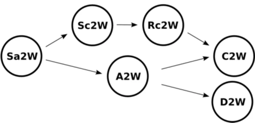
Keeping in mind that the reduction between problems is transitive and re-flexive, this leads to a hierarchy of problems illustrated by the graph in Figure
Figure 2.2: Preordering of the reductions between problems.
2.2. The most general problems is Sa2W, and all other problems reduce to it. Problems D2W and C2W are the most specific. The complete chains in the preordering of the problems are:
C2W ∝ Rc2W ∝ Sc2W ∝ Sa2W C2W ∝ A2W ∝ Sa2W
D2W ∝ A2W ∝ Sa2W
Throwing a rope to the next chapters, it is fundamental to point out that, for the purpose of benchmarking the annotation systems, the performance of
two systems S0 (solving problem P0) and S00(solving problem P00) can be fairly
compared only if they respectively solve P0 and P00, and there is a problem P
such that P ∝ P0 ∧ P ∝ P00. In this hypothesis, the evaluation can be done
with respect to the ability of systems S0 and S00 to solve problem P . Since
the preordering of the reductions is reflexive, obviously two systems can be
compared if they both solve problem P or if they solve respectively P0 and P00,
and P0∝ P00.
Keeping an eye on the graph in Figure 2.2, note that the performances of
systems S0 and S00 in solving problem P can be compared if and only if a
reverse-path exists from problem P to P0 and from problem P to P00.
Also note that, if P0∝ P00, a dataset giving a gold standard (i.e. an expected
output) for P00 can be adapted to be used as a gold standard for P0, using the
2.4
Conclusions
This chapter has presented the basic terminology that will be used in the follow-ing chapters. We also presented the first part of the formal framework, definfollow-ing a set of problems related to topic retrieval. These problems show different fea-tures, but can be framed into a preordering representing the reduction between
them. This lets two systems natively solving two different problems P0 and P00
be fairly compared to each other with respect to their ability to solve a third
Chapter 3
New evaluation metrics
We judge ourselves by what we feel capable of doing, while others judge us by what we have already done.
– Henry Wadsworth Longfellow, Kavanagh: A Tale.
The issue of establishing a baseline, shared by the community, to evaluate the performance of systems that solve the problems presented in Chapter 2 is of crucial importance to help the development of new algorithms and to address the research in this field. In this chapter, some metrics for the evaluation of correctness are proposed. The aim is to establish a set of experiments that fairly evaluate the performance of a system (Section 3.1) and evaluate how similar two systems are (Section 3.4). The performance of a system mainly depends on four factors:
1. The ability of the system in recognizing the mentions (for problems Sa2W and A2W).
2. The ability of the system in assigning a set of candidate concepts to each mention (for problems Sa2W, A2W and D2W) or to the whole text (Sc2W, Rc2W, C2W);
3. The ability of the system in selecting the right concept (disambiguation); 4. The ability of the system in assigning the score (for problems Sc2W,
Sa2W) or the ranking (for Rc2W) to the annotations or tags.
While Section 3.1 presents a set of metrics to evaluate the performance of the full chain of these abilities (1-4) for all problems, some of them can be tested in-depth and separately: Section 3.2 focuses the metrics on the evaluation of finding mentions (ability 1), while metrics presented in Section 3.3 evaluates the ability of finding the right concepts (abilities 2 and 3).
3.1
Metrics for correctness evaluation
Experiments are performed checking the output of the tagging systems against the gold standard given by a dataset. Of course, for each problem a different set of metrics has to be defined. This section covers all the problems presented in Chapter 2. Classical measures like the true positives, false positives, false negatives, precision and recall are generalized and built on top of a set of binary relations. These binary relations represent a match between two tags or two annotations. The necessity of the generalization comes from the need that two annotations or tags, to be considered as matching, do not need to be equal but, more generally, have to satisfy a match relation. Things will be clearer continuing the reading of the next subsections. In the meanwhile, the following definitions are given:
Definition 1 Let X be the set of elements such that a solution of problem P is a subset of X. Let r ⊆ X be the output of the system for an instance I of problem P , g ⊆ X be the gold standard given by the dataset for instance I and M a symmetric match relation on X. The following higher-order functions are defined:
true positives tp(r, g, M ) = {x ∈ r | ∃x0∈ g : M (x0, x)}
false positives f p(r, g, M ) = {x ∈ r | 6 ∃x0∈ g : M (x0, x)}
false negatives f n(r, g, M ) = {x ∈ g | 6 ∃x0∈ r : M (x0, x)}
true negatives tn(r, g, M ) = {x 6∈ r | 6 ∃x0∈ g : M (x0, x)}
Generally, a dataset offers more than one instance. Thus, an output of a system checked against all the instances provided by a dataset consists of a list of results, one for each instance. The following commonly used metrics [26] are re-defined, generalized with the matching relation M .
Definition 2 Let G = [g1, g2, · · · , gn] be the gold standard given by a dataset
that contains n instances I1, · · · , In, given as input to a system, gi being the
gold standard for instance Ii. Let R = [r1, · · · , rn] be the output of the system,
where ri is the result found by the system for instance Ii. The following metrics
precision P (r, g, M ) = |tp(r,g,M )|+|f p(r,g,M )||tp(r,g,M )| recall R(r, g, M ) = |tp(r,g,M )|+|f n(r,g,M )||tp(r,g,M )| F1 F1(r, g, M ) =2·P (r,g,M )·R(r,g,M )P (r,g,M )+R(r,g,M ) macro-precision Pmacro(R, G, M ) = n1·P n i=1P (ri, pi, M )
macro-recall Rmacro(R, G, M ) = 1n·Pni=1R(ri, gi, M )
macro-F1 F 1macro(R, G, M ) = n1 ·P n i=1F1(ri, gi, M ) micro-precision Pmicro(R, G, M ) = Pn i=1|tp(ri,gi,M )| Pn i=1(|tp(ri,gi,M )|+|f p(ri,gi,M )|) micro-recall Rmicro(R, G, M ) = Pn i=1|tp(ri,gi,M )| Pn i=1(|tp(ri,gi,M )|+|f n(ri,gi,M )|) micro-F1 F 1micro(R, G, M ) = 2·Pmicro(R,G,M )·Rmicro(R,G,M ) Pmicro(R,G,M )+Rmicro(R,G,M )
Note that, if the binary relation M is the equality (M (a, b) ⇔ a = b), the measures presented above become the classical Information Retrieval measures. Now that this layer of metrics have been defined, we can play on the match relation M .
3.1.1
Metrics for the C2W problem
For the C2W problem, the match relation to use is quite straightforward. The output of a C2W system is a set of tags. Keeping in mind that a tag is codified as the concept it refers to, the following definitions are given:
Definition 3 Let T be the set of all tags. A Strong tag match is a binary
relation Mton T between two tags t1 and t2. It is defined as
Mt(t1, t2) ⇐⇒ d(t1) = d(t2)
Where d is the dereference function (see Definition 4)
Definition 4 Let L be the set of redirect pages, C be the set of non-redirect pages (thus C ∩ L = ∅) in Wikipedia. Dereference is a function
d : L ∪ C ∪ {null} 7→ C ∪ {null} such that: d(p) = p if p ∈ C p0 if p ∈ L null if p = null
Definition 3 and the dereference function worth an explanation. In Wikipe-dia, a page can be a redirect to another, e.g. “Obama” and “Barrack Hussein Obama” are redirects to “Barack Obama”. Redirects are meant to ease the finding of pages by the Wikipedia users. Redirects can be seen as many-to-one bindings from all synonyms (pages in L) to the most common form of the same
concept (pages in C). Two concepts identified by c1 and c2, where c16= c2but
d(c1) = d(c2) (meaning that c1redirects to c2 or that c1 and c2 redirect to the
same page c3) represent the same concept and thus must be considered as equal.
It is obvious that the Strong tag match relation Mt is reflexive (∀x ∈
T. Mt(x, x)), symmetric (Mt(y, x) ⇔ Mt(x, y)), and transitive (Mt(x, y) ∧
Mt(y, z) ⇒ Mt(x, z)).
To achieve the actual metrics for the C2W problem, the number of true/false positives/negatives, precision, recall and F1 must be computed according to
Definitions 1 and 2, using M = Mt.
3.1.2
Metrics for the D2W problem
D2W output consists of a list of annotations, some of them possibly with null -concept. To compare two annotations, the following match function, as well reflexive, symmetric and transitive, is given.
Definition 5 Let A be the set of all annotations. A Strong annotation match
is a binary relation Ms on A between two annotations a1 = hhp1, l1i, c1i and
a2= hhp2, l2i, c2i . It is defined as Ms(a1, a2) ⇐⇒ p1= p2 l1= l2 d(c1) = d(c2)
Where d is the dereference function (see Definition 4).
Note that in D2W it does not make sense to count the negatives, since the mentions of the annotations contained in the output are the same as the mentions given as input, and only the concepts can be either correct (true positive) or wrong (false positive). To compute the number of true and false positives, as long as the precision, functions defined in Definition 1 and 2 can
be used, with M = Ms.
3.1.3
Metrics for the A2W problem
As in D2W, the output of a A2W problem is a set of annotations. The main difference is that in A2W the mentions are not given as input and must be found by the system.
A possible set of metrics for A2W would be analogue to those given in
Defi-nitions 1 and 2 with M = Ms(Definition 5). But the Strong annotation match
will result to be true only if the mention matches perfectly, and this approach leaves aside some cases of matches that should still be considered as right. Sup-pose a A2W annotator is given as input the sentence “The New Testament is the basis of Christianity”. A correct annotation returned by the annotation system could be hh4, 13i, New Testament i (correctly mapping the mention “New Testa-ment” to the concept New Testament ). But suppose the gold standard given by the dataset was another similar and correct annotation hh0, 17i, New Testament i (mapping the mention “The New Testament” to the same concept). Since the mentions differ, a metric based on the Strong annotation match would count one false positive and one false negative, whereas only one true positive should be counted. Definition 5 can be relaxed as described in Definition 6 to match annotations with overlapping mentions and same concept.
Definition 6 Let A be the infinite set of all annotations. A Weak annotation
match is a binary relation Mw on A between two annotations a1= hhp1, l1i, c1i
and a2= hhp2, l2i, c2i. Let e1= p1+ l1− 1 and e2= p2+ l2− 1 be the indexes
of the last character of the two mentions. The relation is defined as
Mw(a1, a2) ⇐⇒
(
p1≤ p2≤ e1 ∨ p1≤ e2≤ e1 ∨ p2≤ p1≤ e2 ∨ p2≤ e1≤ e2
d(c1) = d(c2)
A Weak annotation match is verified if a Strong annotation match is verified (annotations have equal mentions) or, more generally, if the mentions overlap. Both are verified only if the concept of the annotations is the same. Relation
Mwis trivially reflexive and symmetric, but is not transitive nor anti-symmetric.
Metrics for the A2W problem can be those defined in Definition 1 and 2,
with M = Mw(for Weak annotation match) or M = Ms(for Strong annotation
match).
3.1.4
Metrics for the Rc2W problem
As pointed out in [27], since the output of a Rc2W system is a ranking of tags, common metrics like P1, R-prec, Recall, MRR and MAP [26] should be used
3.1.5
Metrics for the Sc2W and Sa2W problems
As their non-scored version, Sc2W and Sa2W return respectively a set of an-notations and a set of tags, with the addition of a likelihood score for each
annotation/tag. In practice, the output of such systems is never compared
against a gold standard of the same kind (in a gold standard, it’s a nonsense to assign a “likelihood score” to the annotations/tags). Hence, the output of a Sc2W and Sa2W system must be adapted (see the Section 2.3 about problem reductions) to the problem for which a solution is offered by the gold standard. This introduce a threshold on the score. Metrics presented above (Definitions 1
and 2 with M = Mt for Sc2W and M ∈ {Mw, Ms} for Sa2W) can be used for
values of the threshold ranging in [0, 1].
3.2
Finding the mentions (for Sa2W and A2W)
The metrics presented above for Sa2W and A2W measure the ability of the systems to find the correct annotation, which includes, for each annotation, finding both the correct mention and the correct concept. But how much of the error is determined by the lack of mention recognition? To answer this question, we can use a match relation that only checks the overlap of mentions, ignoring the concept:
Definition 7 Let A be the set of all annotations. A Mention annotation match
is a binary relation Mmon set A between two annotations a1= hhp1, l1i, c1i and
a2 = hhp2, l2i, c2i. Let e1 = p1+ l1− 1 and e2 = p2+ l2− 1 be the indexes of
the last character of the two mentions. The relation is defined as
Mm(a1, a2) ⇐⇒ p1≤ p2≤ e1 ∨ p1≤ e2≤ e1 ∨ p2≤ p1≤ e2 ∨ p2≤ e1≤ e2
3.3
Finding the concepts (for Sa2W and A2W)
Dually, it would be interesting, when comparing the result of a Sa2W/A2W problem against a gold standard, to isolate the problem of finding the right con-cepts (discarding the binding of the mentions to the concon-cepts). That’s exactly what is done by the metrics for the C2W problem presented above.
Hence, to isolate the measure of concept recognition, the output of a system, as long as the gold standard, have to be adapted to a solution for the C2W problem (See Table 2.3) and measured with metrics presented in 3.1.1.
1. Adapt the Sa2W output to a A2W output choosing a score threshold under which annotations are discarded (Sa2W only);
2. Discard annotations a = (p, l, c) ∈ Ad given for document d such that
∃a0 = (p0, l0, d0) ∈ A
d | a0 6= a ∧ d(c) = d(c0) (i.e. if more than one
annotation have the same concept, keep only one of them);
3. Use the metrics defined in Definitions 1 and 2 with M = Mc, defined as:
Definition 8 Let A be the set of all annotations. A Concept annotation match
is a binary relation Mc on A between two annotations a1 = hp1, l1, c1i and
a2= hp2, l2, c2i. It is defined as
Mc(a1, a2) ⇐⇒ d(c1) = d(c2)
Where d is the dereference function (see Definition 4)
This measure roughly reflects the performance of the candidate finding and the disambiguation process, and is fundamental for all applications in which we are interested in retrieving the concept a text is about, rather than the annotations.
3.4
Similarity between systems
The similarity between systems can be measured considering how similar their output for the text documents contained in a dataset are. In this section, the
following definitions hold: let D = [d1, d2, · · · , dn] be a dataset that contains
n documents, given as input to two systems t1 and t2 that solve problem P ∈
{Sa2W, Sc2W, Rc2W, C2W, A2W, D2W}. Let A = [a1, a2, · · · , an] and B =
[b1, b2, · · · , bn] be respectively the output of t1 and t2, so that ai and bi are the
solutions found respectively by t1and t2for document di. The type of elements
in A, that is the same as elements in B, varies depending on the problem P that t1 and t2 solve.
3.4.1
A new similarity measure on sets
A proposed measure to check the similarity of the two sets of annotations a and b is inspired by the Jaccard similarity coefficient [21], but must take into account the possibility that two annotations match according to a match relation such as those presented in Definitions 3, 5, 6, 7 and 8, even though not being equal. The following measure is proposed:
Definition 9 Let a ⊆ X and b ⊆ X be two sets, and M be a reflexive and
symmetric relation on set X. Similarity measure S0 is defined as:
S0(a, b, M ) = |{x ∈ a | ∃y ∈ b : M (x, y)}| + |{x ∈ b | ∃y ∈ a : M (x, y)}|
|a| + |b|
Note that function S0 is symmetric and ranges in [0, 1]. Important features
of S0 are that S0(a, b) = 1 if and only if, for all elements in a, there is a matching
element in b, and vice-versa; S0(a, b) = 0 if and only if there is not one single
element in a that matches with an element in b, and vice-versa. Unlike the
Jaccard measure, S0 is not a distance function since S0(a, b) = 0 does not imply
a = b, and it does not verify the triangle inequality.
Note that for our purpose, as M , any of Strong tag match (for Sc2W and C2W systems whose output is a set of tags), Weak annotation match, Strong annotation match, Mention annotation match and Concept annotation match (for Sa2W, A2W, D2W systems whose output is a set of annotations) can be used, since they are all reflexive and symmetric.
3.4.2
A similarity measure on lists of sets
The similarity of two lists of sets A and B can be defined as the average of S0on
the sets of the lists, giving the same importance to all the sets contained in the
lists regardless of their size (Smacro) or as the overall “intersection” divided by
the overall size, which gives more importance to bigger sets (Smicro). Formally:
Definition 10 Let A and B be two lists of elements ai, bi⊆ X and let M be a
binary relation on X. The following definitions are given: Smacro(A, B, M ) = n1·P
n
i=1S0(ai, bi, M )
Smicro(A, B, M ) = Pn
i=1(|{x∈ai | ∃y∈bi: M (x,y)}|+|{x∈bi | ∃y∈ai: M (x,y)}|)
Pn
i=1(|ai|+|bi|)
Smacro and Smicro share the same properties as S0: they range in [0, 1],
their value is 0 if and only if, for each i ∈ [1, · · · , n], there is not one single
element in ai that matches with an element in biand vice-versa, and their value
is 1 if and only if, for each i ∈ [1, · · · , n] and for all elements in ai, there is
a matching element in bi, and vice-versa. If M is reflexive and A = B, then
3.4.3
Combining S with M
∗Let S be any of Smacro or Smacro. The meaning of the value given by this
similarity measure depends only on the match relation M it is combined with.
For C2W and Sc2W, the only defined matching function is M = Mt. In this
case, S give a measure of how many of the concepts found by t1 and t2 are in
common.
For all problems whose output is a set of annotations (Sa2W, A2W, D2W),
any match relation M ∈ {Ms, Mw, Mm, Mc} can be used, with the following
meaning:
• S(A, B, Ms) gives the fraction of common annotations (having same
con-cept and same mention).
• S(A, B, Mw) gives the fraction of common overlapping annotations
(hav-ing same concept and overlapp(hav-ing mention).
• S(A, B, Mm) gives the fraction of common overlapping mentions found in
the text.
• S(A, B, Mc) gives the fraction of common concepts found in the text.
3.4.4
Measuring true positives and true negatives
similar-ity in detail
S-measures can be used not only to check the whole output of two systems. The focus can instead be put on measuring how many of the true positives and true negatives two systems have in common, to see whether their correct spots and mistakes are similar or not. To do this, we can simply take a subset of elements of A and B representing the true positives or the false negatives.
Definition 11 Let G = [g1, · · · , gn] be the gold standard for a dataset, gi⊆ X
being the gold standard for instance Ii. Let O = [o1, · · · , on] be the output of
a system, oi ⊆ X being the output for instance Ii. Let M be a reflexive and
symmetric binary relation on X. The following definitions are given: T (O, G, M ) = [tp(o1, g1, M ), · · · , tp(on, gn, M )]
F (O, G, M ) = [f p(o1, g1, M ), · · · , f p(on, gn, M )]
Where tp and f p are the true positives and the false positives functions defined in Definition 1.
T (O, G, M ) and F (O, G, M ) are lists containing, for each instance Ii,
re-spectively the true positives and the false positives contained in the output oi
The fraction of common true positives between outputs A and B is hence given by S(T (A, G, M ), T (B, G, M ), M ) whereas the fraction of common false negatives is given by S(F (A, G, M ), F (B, G, M ), M ), where S can be either Smicro or Smacro.
3.5
Conclusions
This chapter has presented the second part constituting the formal framework employed in this thesis. The classical measures of Information Retrieval have been generalized adding a match relation M . This includes the basic measure-ment of true/false positives/negatives for the solution of a single instance and the F1, precision and recall measurements, in their macro- and micro- version, for a set of solutions to instances given, for example, by a dataset. M is a binary relation defined on a generic set X such that the output of a system is formed by a subset of X. Playing on M , we can focus the measurement on specific fea-tures of the comparison. For every problem, we defined a proper match relation that, combined with the defined measures, lets us evaluate the performance of a system in solving that problem. Other proposed match relations let us focus the measures on certain aspects of a system.
We also defined a way of comparing the output of two systems, as well based on a match relation. This S measure is inspired by the Jaccard similarity measure but takes as parameter a match relation M . The similarity can be restricted to the true positives or the false positives using functions T and F .
Chapter 4
The comparison framework
Comparisons are odious.– Archbishop Boiardo, Orlando Innamorato.
It has been developed a benchmarking framework that runs experiments on systems that solve problems given in Chapter 2 in order to measure the performance of the systems and their similarity. The framework is based on the metrics given in Chapter 3, providing an implementation of the proposed measures and match relations. The target was to create a framework that is easily extendible with new problems, new annotation systems, new datasets, new match relations and new metrics not yet defined. This work is intended to be released to the public, as a contribution to the scientific community working on the field of topic retrieval. We would like it to become a basis for further experiments, that anyone can reproduce on its own. Distributing this work open source and with a clear documentation is a condition to let anyone assess its fairness or propose modifications to the code.
The framework is written in Java and implements the actual execution of the systems on a given dataset, the caching of the results, the measuring of the performance in terms of correctness and runtime against a given dataset, the computation of the similarity between systems, the reduction between problems
(that is, given two problems P0, P00 such that P0 ∝ P00, adapting an instance
of P0 to P00 and adapt the solution of P00 to P0). Datasets and topic-retrieval
systems are implemented as plugins.
4.1
Code structure
The code of the comparison framework is organized in 8 Java packages. All package names begin with it.acubelab.annotatorBenchmark:
.data contains classes representing basic objects needed by the framework: Annotation, ScoredAnnotation, Tag, ScoredTag.
.cache contains the caching system for the results of the experiment. Caching is needed to avoid the repetition of experiments that may last for days, depending on the size of the dataset. The package also contains, in class Benchmark, the core of the framework, namely the methods to actually perform the experiments and store the results in the cache. Caching is done by simply storing the result in an object of the class BenchmarkResults and serializing it to a file.
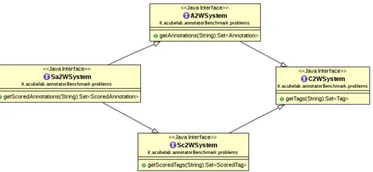
.problems contains interfaces representing a dataset for the problems defined in Chapter 2 (such interfaces are called P Dataset, where P is the name of the problem, E.g. A2WDataset, C2WDataset) and the interfaces for a system
solving one of them (called P System, E.g. A2WSystem, C2WSystem)1. The
class hierarchy reflects the preordering of the problems given in Figure 2.2: if P ∝ Q then a system that solve Q can as well solve P . Speaking of interfaces, this is reflected in the fact that a system that implements interface QSystem (which defines a method for solving an instance of Q) must also implement methods in P System (which defines a method for
solving an instance of P ), and thus QSystem extends P System. The
hierarchy of these classes is reported in Figure 4.2.
.datasetPlugins contains some implementations of P Dataset interfaces of package .problems. These classes provide standard datasets used in lit-erature.
.systemPlugins contains some implementations of P System interfaces of pack-age .problems, providing actual access to the topic-retrieval systems. These classes are the glue between the benchmarking framework and the topic-retrieval systems. Generally, in their implementation, to solve an instance of a problem, they query the system through its web service or running it locally.
.metrics contains the implementation of the metrics presented in Chapter 3. The abstract class Metrics provides the methods for finding the true/false positives/negatives and for computing precision, recall, F1 and similarity. These methods need, as parameter, an object representing a match rela-tion, like those given in Section 3.1. The implementations of the match relations (StrongTagMatch, StrongAnnotationMatch, etc.) are as well 1Interfaces for problems for which there is no system (natively or not) solving it or datasets giving a gold standard for it, were not implemented in this version of the benchmarking framework. They will be added if needed.
Figure 4.1: Automatically-generated UML class diagram with the packages of the annotator benchmark framework and their dependencies.
contained in this package. Classes representing a match relation on type E implement the generic interface MatchRelation, using E as type param-eter.
.utils contains some general-purpose utilities used along the whole frame-work. This includes some Exceptions; some data-storing utilities; Export, the utility to export a dataset in XML form; ProblemReduction that im-plements the adaptations of instances and solutions needed for problem reductions; and WikipediaApiInterface, that provides some methods to query the Wikipedia API to retrieve information about concepts (Wikipe-dia pages). In particular, Wikipe(Wikipe-diaApiInterface.dereference(int) implements the de-reference function d defined in Definition 4.
.scripts contains example scripts that run the benchmark on the datasets and
print data in gnuplot and LATEX style.
The packages form a kind of four-“layer” structure2, depicted in Figure 4.1.
At the two bottom layers lie the utility package and the data package, sparsely used by all other packages. The third layer provides the abstract part of the framework, including the interfaces and the implementation of the metrics mea-surement. The fourth and most concrete layer provide both the caching and the implementations of some datasets and systems.
2The layer term is abused, since packages in the upper layer may depend on all lower layers, and not only on the layer just below.
Figure 4.2: Hierarchy of interfaces that topic annotators must implement, re-flecting the hierarchy of the problems presented in 2.2.
4.2
Running the experiments
A class with a main() method running the actual experiments should be located on top of all these packages. The main() method basically creates the objects representing the topic-retrieval system, the dataset, the match relation and the metrics, asks the cache for the result for each document of the dataset (the cache will perform the experiment if the result is not cached), and outputs the results given by the metrics. An example snippet of code follows.
1 p u b l i c c l a s s L u l z M a i n { 2
3 p u b l i c s t a t i c v o i d m a i n(S t r i n g[] a r g s) { 4 B e n c h m a r k.u s e C a c h e(" r e s u l t s . c a c h e ") ;
5 W i k i p e d i a A p i I n t e r f a c e api = new W i k i p e d i a A p i I n t e r f a c e(" wid . c a c h e ", " r e d i r e c t . c a c h e ") ;
6 M a t c h R e l a t i o n<A n n o t a t i o n> wam = new W e a k A n n o t a t i o n M a t c h(api) ; 7 Metrics<A n n o t a t i o n> m e t r i c s = new Metrics<A n n o t a t i o n>() ; 8 S a 2 W S y s t e m m i n e r = new W i k i p e d i a M i n e r A n n o t a t o r() ;
9 A 2 W D a t a s e t a i d a D s = new C o n l l A i d a D a t a s e t(" d a t a s e t s / a i d a / AIDA YAGO2 -d a t a s e t . tsv ", api) ; 10 11 List<Set<S c o r e d A n n o t a t i o n> > c o m p u t e d A n n o t a t i o n s = B e n c h m a r k. d o S a 2 W A n n o t a t i o n s(miner, a i d a D s) ; 12 List<Set<A n n o t a t i o n> > r e d u c e d A n n o t a t i o n s = P r o b l e m R e d u c t i o n. S a 2 W T o A 2 W L i s t(c o m p u t e d A n n o t a t i o n s, 0.5f) ; 13 List<Set<A n n o t a t i o n> > g o l d S t a n d a r d = a i d a D s.g e t A 2 W G o l d S t a n d a r d L i s t() ; 14 M e t r i c s R e s u l t S e t rs = m e t r i c s.g e t R e s u l t(r e d u c e d A n n o t a t i o n s, g o l d S t a n d a r d, wam) ; 15 16 p r i n t R e s u l t s(rs) ; 17 18 B e n c h m a r k.f l u s h() ; 19 api.f l u s h() ; 20 }
Figure 4.3: Main classes and interfaces involved in running the Wikipedia Miner annotator on the Conll/AIDA dataset. Both system and dataset will be pre-sented in Chapter 5
21
22 p u b l i c s t a t i c v o i d p r i n t R e s u l t s(M e t r i c s R e s u l t S e t rs) { 23 // p r i n t t h e r e s u l t s
24 } 25 }
Let’s have a closer look at the snippet of code above. Figure 4.3 shows the hierarchy of the classes and interfaces involved in this snippet. Lines 4-9 prepare the environment: the cache containing the results of the problems is bound to file results.cache. An object representing the API to Wikipedia is created and assigned to variable api. This object is needed by the match method of the WeakAnnotationMatch object, assigned to variable wam, that implements the Weak annotation match: as defined in Definition 6, this match relation is based on the dereference function, implemented by the Wikipedia API. An object representing the Wikipedia Miner annotator – discussed in Chapter 5 – is created and assigned to variable miner. In the implementation, this object queries the Wikipedia Miner web service passing a document as parameter and
returning the resulting set of scored annotations. Furthermore, the dataset
AIDA/CoNLL is created, loading the instances (i.e. documents) and the gold standard from a file.
Lines 11-14 call some methods to gather the actual output of the Wikipedia Miner system for the dataset AIDA/CoNLL. If this system has already been called for some of the text contained in the dataset, the result stored in the cache will be quickly returned instead of calling the Wikipedia Miner web service. Since Wikipedia Miner solve problem Sa2W, while the dataset represent a gold standard for problem A2W, the output of Wikipedia Miner (for each document, a set of scored annotations) must be adapted to the output of A2W, discarding the scores and taking only the annotations above a given threshold. In the code snippet, the adaption of the solution is done in line 12 and the threshold on the score is set to 0.5. In line 14 the object representing the metrics is called, passing as parameter the list of solutions adapted to A2W, the A2W gold standard given by the dataset, and the Weak annotation match object. The metrics object computes the actual measures like the true positives, the precision, the F1, etc. Results are returned in an object of class MetricsResultSet whose content is printed to the screen calling method printResults in line 16.
Lines 18-19 flush the cache of the results and of the Wikipedia API to a file in a permanent memory, to guarantee a faster execution if the Main method is executed twice.
4.3
Extending the framework
An important feature of this benchmarking framework is that it can be easily extended with new problems, new annotation systems, new datasets, new match relations and new metrics. Let’s have a closer look at how an implementation should be done for each of these categories.
4.3.1
Extending with new systems
To add to the framework a new system that solves a problem A, all that is needed is to create a class that implements interface ASystem. Note that a single system may natively solve more than one problem. In this case, the class will implement one interface for each problem solved.
Suppose we want to add a new system called Cool Annotator that natively solve A, and let B be a problem such that B ∝ A that Cool Annotator does not natively solve. Let CoolAnnotator the concrete class representing the system, implementing ASystem (and thus BSystem). CoolAnnotator will implement a method defined in ASystem to solve problem A. The implementation of the method defined in BSystem to solve problem B should simply
1. call routine methods to adapt the instance IB of problem B to an instance
IA of problem A. This takes polynomial time;
2. call the method defined in ASystem for solving problem A on the instance IA, it will return solution SA;
3. adapt SA to a solution SB of problem B. This takes polynomial time;
4. return SB.
Methods for adapting the instances and the solutions from a problem to another are implemented in the class ProblemReductions in package utils. Here follows a complete example for A = A2W, B = T2W (thus, the reduction is T2W ∝ A2W). The following interfaces are involved:
Interface problems.C2WSystem: 1 p u b l i c i n t e r f a c e C 2 W S y s t e m e x t e n d s T o p i c S y s t e m { 2 p u b l i c Set<Tag> s o l v e C 2 W(S t r i n g t e x t) t h r o w s A n n o t a t i o n E x c e p t i o n; 3 } Interface problems.A2WSystem: 1 p u b l i c i n t e r f a c e A 2 W S y s t e m e x t e n d s C 2 W S y s t e m{ 2 p u b l i c Set<A n n o t a t i o n> s o l v e A 2 W(S t r i n g t e x t) t h r o w s A n n o t a t i o n E x c e p t i o n ; 3 }
A draft for an annotator natively solving A2W (and thus solving C2W as well), implementing the A2WSystem interface specified above, could look like this: 1 p u b l i c c l a s s C o o l A n n o t a t o r i m p l e m e n t s A 2 W S y s t e m{ 2 p r i v a t e l o n g l a s t T i m e = -1; 3 4 @ O v e r r i d e 5 p u b l i c Set<A n n o t a t i o n> s o l v e A 2 W(S t r i n g t e x t) { 6 l a s t T i m e = C a l e n d a r.g e t I n s t a n c e() .g e t T i m e I n M i l l i s() ; 7 Set<A n n o t a t i o n> r e s u l t = t h i s.c o m p u t e R e s u l t(t e x t) ; 8 l a s t T i m e = C a l e n d a r.g e t I n s t a n c e() .g e t T i m e I n M i l l i s() - l a s t T i m e; 9 r e t u r n r e s u l t; 10 } 11 12 @ O v e r r i d e 13 p u b l i c Set<Tag> s o l v e C 2 W(S t r i n g t e x t) t h r o w s A n n o t a t i o n E x c e p t i o n { 14 // no a d a p t a t i o n of t h e i n s t a n c e is n e e d e d 15 Set<A n n o t a t i o n> t a g s = s o l v e A 2 W(t e x t) ; 16 r e t u r n P r o b l e m R e d u c t i o n.A 2 W T o C 2 W(t a g s) ; 17 } 18 19 @ O v e r r i d e 20 p u b l i c S t r i n g g e t N a m e() { 21 r e t u r n " C o o l A n n o t a t o r "; 22 } 23 24 @ O v e r r i d e 25 p u b l i c l o n g g e t L a s t A n n o t a t i o n T i m e() { 26 r e t u r n l a s t T i m e; 27 } 28 29 p r i v a t e Set<A n n o t a t i o n> c o m p u t e R e s u l t(S t r i n g t e x t) { 30 // do t h e a c t u a l a n n o t a t i o n s 31 } 32 }
Method solveA2W() is the method which is called for annotating a doc-ument. In its body, it takes the time after and before the annotation pro-cess and store the difference in the lastTime variable returned by
getLast-AnnotationTime(). The actual annotations are done by a private method
computeResult().
Method solveC2W() gives the solution for problem C2W. Since an instance for problem C2W (a text) is also an instance for problem A2W, there is no need to adapt it. The instance is therefore solved for problem A2W calling the method solveA2W(). Its solution is then adapted to a solution of the C2W problem, calling ProblemReduction.A2WToC2W(). In its body (not listed), this method simply discards the mentions leaving the computed concepts.
4.3.2
Extending with new datasets
To add to the framework a new dataset giving a gold standard for problem A, all that is needed is to make a concrete class C implementing interface ADataset. Talking of inheritance, the same logic explained in previous subsections for the system hierarchy holds for the dataset hierarchy. A complete example of two interfaces C2WDataset and A2WDataset follows. Note that C2W ∝ A2W (see Chapter 2).
Interface problems.C2WDataset:
1 p u b l i c i n t e r f a c e C 2 W D a t a s e t e x t e n d s T o p i c D a t a s e t{ 2 p u b l i c List<String> g e t T e x t I n s t a n c e L i s t() ; 3 p u b l i c List<Set<Tag> > g e t C 2 W G o l d S t a n d a r d L i s t() ; 4 p u b l i c int g e t T a g s C o u n t() ; 5 } Interface problems.A2WDataset: 1 p u b l i c i n t e r f a c e A 2 W D a t a s e t e x t e n d s C 2 W D a t a s e t{ 2 p u b l i c List<Set<A n n o t a t i o n> > g e t A 2 W G o l d S t a n d a r d L i s t() ; 3 }
A draft for a dataset, whose name is Lulz Dataset, implementing the A2WDataset interface specified above, could look like this:
1 p u b l i c c l a s s L u l z D a t a s e t i m p l e m e n t s A 2 W D a t a s e t{ 2 List<String> t e x t s; 3 List<Set<A n n o t a t i o n> > a n n o t a t i o n s; 4 5 p u b l i c L u l z D a t a s e t() t h r o w s A n n o t a t i o n E x c e p t i o n{ 6 t e x t s = t h i s.l o a d T e x t s() ; 7 a n n o t a t i o n s = t h i s.l o a d A n n o t a t i o n s() ; 8 } 9 10 @ O v e r r i d e 11 p u b l i c int g e t S i z e() { 12 r e t u r n t e x t s.s i z e() ; 13 } 14 15 @ O v e r r i d e 16 p u b l i c int g e t T a g s C o u n t() { 17 int c o u n t = 0; 18 for (Set<A n n o t a t i o n> a : a n n o t a t i o n s) 19 c o u n t += a.s i z e() ; 20 r e t u r n c o u n t; 21 } 22 23 @ O v e r r i d e 24 p u b l i c I t e r a t o r<Set<A n n o t a t i o n> > g e t A n n o t a t i o n s I t e r a t o r() { 25 r e t u r n a n n o t a t i o n s.i t e r a t o r() ; 26 } 27 28 @ O v e r r i d e 29 p u b l i c List<Set<A n n o t a t i o n> > g e t A 2 W G o l d S t a n d a r d L i s t() { 30 r e t u r n a n n o t a t i o n s; 31 }
32 33 @ O v e r r i d e 34 p u b l i c List<String> g e t T e x t I n s t a n c e L i s t() { 35 r e t u r n t e x t s; 36 } 37 38 @ O v e r r i d e
39 p u b l i c List<Set<Tag> > g e t C 2 W G o l d S t a n d a r d L i s t() {
40 r e t u r n P r o b l e m R e d u c t i o n.A 2 W T o C 2 W L i s t(t h i s.g e t A 2 W G o l d S t a n d a r d L i s t() ) ; 41 } 42 43 @ O v e r r i d e 44 p u b l i c S t r i n g g e t N a m e() { 45 r e t u r n " L u l z D a t a s e t "; 46 } 47 48 p r i v a t e List<String> l o a d T e x t s() { 49 // l o a d t h e t e x t d o c u m e n t s f r o m s o m e w h e r e i n t o v a r i a b l e t e x t s 50 } 51 52 p r i v a t e List<Set<A n n o t a t i o n> > l o a d A n n o t a t i o n s() { 53 // l o a d t h e a n n o t a t i o n s f o r t h e d o c u m e n t s f r o m s o m e w h e r e i n t o v a r i a b l e a n n o t a t i o n s 54 }
4.3.3
Extending the hierarchy of problems
Suppose we want to add a problem A. The hierarchy of interfaces – one for each problem – presented in Figure 4.2, can be extended adding a new interface called ASystem that all systems solving A must implement, providing methods to solve an instance of A.
This interface should extend interface BSystem of package problems if and only if B ∝ A. In this hypothesis, a class implementing ASystem representing a system that solves the harder-problem A, must also implement the methods defined in BSystem (therefore, it must also be able to solve the easier problem B, as by the hypothesis B ∝ A).
Moreover, the hierarchy of interfaces for datasets, that is isomorphic to the hierarchy for the systems interfaces, can be extended in an analogous way, adding interface ADataset that extends BDataset if and only if B ∝ A.
Let B ∝ A. As explained in the previous subsections, to let a system natively solving A solve B as well, a polinomial-time algorithm to adapt an instance of B to an instance of A and a polinomial-time algorithm to adapt the solution of A to a solution of B must be implemented. Two methods performing these two adaptions must be implemented in a class extending ProblemReduction in package utils.
A complete example follows. Suppose we want to add Ab2W (defined in Definition 13 and further detailed in Chapter 7) to the problem hierarchy. Ab2W
is the problem of finding both mentioned concepts expressed in a text (like in Sa2W) and the concepts expressed in a text, even though being not mentioned. For an example, see Chapter 7. The solution of the problem is thus formed by
two sets: sa is the set of scored annotations (for mentioned concepts) and st is
the set of scored tags (for non-mentioned concepts). It’s trivial that Sa2W ∝ Ab2W: the instance needs no adaptation and the solution of Ab2W can be
adapted to Sa2W simply discarding stand keeping sa.
The new interface representing a system that solve Ab2W would look like the following. Method getAb2WOutput returns a solution for problem Ab2W:
1 p u b l i c i n t e r f a c e A b 2 W S y s t e m e x t e n d s S a 2 W S y s t e m{
2 p u b l i c Pair<Set<S c o r e d A n n o t a t i o n> , Set<S c o r e d T a g> > g e t A b 2 W O u t p u t(S t r i n g t e x t) ;
3 }
The adaptation of the solution is trivially implemented in a method of a class extending ProblemReduction:
1 p u b l i c c l a s s A b 2 W P r o b l e m s R e d u c t i o n e x t e n d s P r o b l e m R e d u c t i o n{ 2 p u b l i c s t a t i c Set<S c o r e d A n n o t a t i o n> A b 2 W T o S a 2 W(Pair<Set<
S c o r e d A n n o t a t i o n> , Set<S c o r e d T a g> > a b 2 w S o l u t i o n) { 3 r e t u r n a b 2 w S o l u t i o n.o u t p u t 1;
4 } 5 }
Here follows the draft of a class representing a system that solves Ab2W. The class implements Ab2WSystem, and thus must provide an implementation for the method getAb2WOutput. The actual solution, computed by the private method computeMentionedAnnotations, is obviously not listed in the exam-ple. Since Sa2W ∝ Ab2W, the class also implements method solveSa2W, that provides a solution for Sa2W, computed calling the method implemented in Ab2WProblemsReduction. All other problems P that this system does not solve natively but such that P ∝ Ab2W, have an analogous method.
1 p u b l i c c l a s s L o l A b s t r a c t A n n o t a t o r i m p l e m e n t s A b 2 W S y s t e m{ 2 p r i v a t e l o n g l a s t A n n o t a t i o n = -1;
3
4 @ O v e r r i d e
5 p u b l i c Pair<Set<S c o r e d A n n o t a t i o n> ,Set<S c o r e d T a g> > g e t A b 2 W O u t p u t(S t r i n g t e x t) {
6 l a s t A n n o t a t i o n = C a l e n d a r.g e t I n s t a n c e() .g e t T i m e I n M i l l i s() ;
7 Pair<Set<S c o r e d A n n o t a t i o n> ,Set<S c o r e d T a g> > res = c o m p u t e A b 2 w S o l u t i o n
(t e x t) ; 8 l a s t A n n o t a t i o n = C a l e n d a r.g e t I n s t a n c e() .g e t T i m e I n M i l l i s() -l a s t A n n o t a t i o n; 9 r e t u r n res; 10 } 11
12 p r i v a t e Pair<Set<S c o r e d A n n o t a t i o n> ,Set<S c o r e d T a g> > c o m p u t e A b 2 w S o l u t i o n(
S t r i n g t e x t) {
13 ... // c o m p u t e t h e s o l u t i o n a n d r e t u r n it .
15 16 @ O v e r r i d e 17 p u b l i c Set<S c o r e d A n n o t a t i o n> s o l v e S a 2 W(S t r i n g t e x t) { 18 r e t u r n A b 2 W P r o b l e m s R e d u c t i o n.A b 2 W T o S a 2 W(g e t A b 2 W O u t p u t(t e x t) ) ; 19 } 20 21 @ O v e r r i d e 22 p u b l i c Set<S c o r e d T a g> s o l v e S c 2 W(S t r i n g t e x t) { 23 r e t u r n A b 2 W P r o b l e m s R e d u c t i o n.S a 2 W T o S t 2 W(s o l v e S a 2 W(t e x t) ) ; 24 } 25 26 @ O v e r r i d e 27 p u b l i c Set<A n n o t a t i o n> s o l v e A 2 W(S t r i n g t e x t) { 28 r e t u r n A b 2 W P r o b l e m s R e d u c t i o n.S a 2 W T o A 2 W(s o l v e S a 2 W(t e x t) ) ; 29 } 30 31 @ O v e r r i d e 32 p u b l i c Set<Tag> s o l v e C 2 W(S t r i n g t e x t) { 33 r e t u r n A b 2 W P r o b l e m s R e d u c t i o n.A 2 W T o C 2 W(s o l v e A 2 W(t e x t) ) ; 34 } 35 36 @ O v e r r i d e 37 p u b l i c S t r i n g g e t N a m e() { 38 r e t u r n " Lol A b s t r a c t A n n o t a t o r "; 39 } 40 41 @ O v e r r i d e 42 p u b l i c l o n g g e t L a s t A n n o t a t i o n T i m e() { 43 r e t u r n l a s t A n n o t a t i o n; 44 } 45 }
4.3.4
Implementation of the metrics
To introduce the extension of the metrics, we first have to explain how the classes involved in the metrics measurement ineract with each other.
Package metrics contains class Metrics which implements the measures defined in Chapter 3 (precision, recall, F1, etc). All methods for computing such metrics take as argument a match relation M , implemented as an object of type MatchRelation. For each match relation M given in Chapter 3, there is a class implementing the interface MatchRelation that provides an implementation of M in the method match.
Class Metrics is generic in that it has type variable T such that the measures are computed over systems that return sets of objects of type T (E.g. T can be Tag, Annotation, etc.). Therefore, measures like micro- and macro- F1, recall and precision are performed for lists of sets of T-objects (a set for each instance given by a dataset). Also interface MatchRelation has generic type variable E, such that the match test is done on elements of type E. Of course, to use a MatchRelation<E> with Metrics<T>, it must be T = E.
• Match relation M is defined on elements of set X (E.g. X can be the set of all annotations);
• Metrics are measured employing M as match relation, thus the tp, fp, fn, F1, recall and precision measures are performed over subsets of X, while micro- and macro- F1, precision and recall are performed over lists
of subsets of X (E.g. M can be the Weak annotation match Mw);
• In the framework, elements of X are represented as objects of class T (E.g. T is class Annotation);
• The match relation M is represented as an object of a class implementing MatchRelation<E>, let this object be assigned to variable matchRelation; • The metrics are represented as an object of a class Metrics<T>, let this
object be assigned to variable metricsComputer; • T=E;
In this scenario, actual measurements using match relation M can be run calling the methods of the metricsComputer and passing matchRelation as argument.
Interface MatchRelation also declares methods preProcessOutput and pre-ProcessGoldStandard, which are called by all methods of class Metrics that implement the measurements, before running the measurements. They should be used if certain metrics need to adapt the output or to perform optimization tasks3.
Before showing the classes, some preparatory speculations must be done. Some gold standards, as well as the output of some annotators, may contain, for a document, annotations with overlapping or nested mentions. For example, the
sentence “A cargo ship is sailing” could contain both annotations a1= hh2, 10i,
Cargo shipi and a2 = hh8, 4i, Shipi. Since some annotation systems return
overlapping annotations while other don’t, comparing the output of an anno-tation system which contains overlapping annoanno-tations against a gold standard that doesn’t contain overlapping annotations (or vice-versa) would be unfair. For the sake of simplicity, before comparing the output of an annotator against a gold standard, in the current implementation of the match relations, both are pre-processed and scanned for overlapping mentions: if two annotations overlap, then only the one with the longest mention is kept, while the other is discarded. The choice of keeping the longest mention is motivated by the assumption that longer mentions refer to more specific – and thus more relevant – concepts (see 3If no pre-processing has to be done, these methods should simply return the data given as parameter.
the example of “Cargo ship” against “Ship”). Note that, using metrics based on Weak annotation match, annotations with longer mentions are more likely to result as a true positive.
Here follows the listing of (parts of) some classes involved in the extension of the metrics.
Class metrics.Metrics implements the measures presented in Chapter 3:
1 p u b l i c c l a s s M e t r i c s <T> { 2
3 p u b l i c M e t r i c s R e s u l t S e t g e t R e s u l t(List<Set<T> > o u t p u t O r i g, List<Set<T> >
g o l d S t a n d a r d O r i g, M a t c h R e l a t i o n<T> m) { 4 List<Set<T> > o u t p u t = m.p r e P r o c e s s O u t p u t(o u t p u t O r i g) ; 5 List<Set<T> > g o l d S t a n d a r d = m.p r e P r o c e s s G o l d S t a n d a r d(g o l d S t a n d a r d O r i g ) ; 6 7 int tp = t p C o u n t(g o l d S t a n d a r d, output, m) ; 8 int fp = f p C o u n t(g o l d S t a n d a r d, output, m) ; 9 int fn = f n C o u n t(g o l d S t a n d a r d, output, m) ; 10 f l o a t m i c r o P r e c i s i o n = p r e c i s i o n(tp, fp) ; 11 f l o a t m i c r o R e c a l l = r e c a l l(tp, fp, fn) ; 12 f l o a t m i c r o F 1 = F1(m i c r o R e c a l l, m i c r o P r e c i s i o n) ; 13 int[] tps = s i n g l e T p C o u n t(g o l d S t a n d a r d, output, m) ; 14 int[] fps = s i n g l e F p C o u n t(g o l d S t a n d a r d, output, m) ; 15 int[] fns = s i n g l e F n C o u n t(g o l d S t a n d a r d, output, m) ; 16 f l o a t m a c r o P r e c i s i o n = m a c r o P r e c i s i o n(tps, fps) ; 17 f l o a t m a c r o R e c a l l = m a c r o R e c a l l(tps, fps, fns) ; 18 f l o a t m a c r o F 1 = m a c r o F 1(tps, fps, fns) ; 19 20 r e t u r n new M e t r i c s R e s u l t S e t(microF1, m i c r o R e c a l l, m i c r o P r e c i s i o n, macroF1, m a c r o R e c a l l, m a c r o P r e c i s i o n, tp, fn, fp) ; 21 } 22 23 p u b l i c s t a t i c f l o a t p r e c i s i o n(int tp, int fp) { 24 r e t u r n tp+fp == 0 ? 1 : (f l o a t)tp/(f l o a t) (tp+fp) ; 25 } 26
27 p u b l i c s t a t i c f l o a t r e c a l l(int tp, int fp, int fn) { 28 r e t u r n fn == 0 ? 1 : (f l o a t)tp/(f l o a t) (fn+tp) ; 29 } 30 31 p u b l i c s t a t i c f l o a t F1(f l o a t recall, f l o a t p r e c i s i o n) { 32 r e t u r n (r e c a l l+p r e c i s i o n == 0) ? 0 : 2*r e c a l l*p r e c i s i o n/(r e c a l l+ p r e c i s i o n) ; 33 } 34
35 p u b l i c List<Set<T> > g e t T p(List<Set<T> > e x p e c t e d R e s u l t, List<Set<T> >
c o m p u t e d R e s u l t, M a t c h R e l a t i o n<T> m) { 36 List<Set<T> > tp = new Vector<Set<T> >() ; 37 for (int i=0; i<e x p e c t e d R e s u l t.s i z e() ; i++) { 38 Set<T> exp = e x p e c t e d R e s u l t.get(i) ; 39 Set<T> c o m p = c o m p u t e d R e s u l t.get(i) ; 40 tp.add(g e t S i n g l e T p(exp, comp, m) ) ; 41 }
42 r e t u r n tp; 43 }
44 45 ...
46 47 }
Class metrics.WeakAnnotationMatch implements the Weak Annotation Match
Mw defined in Definition 6. Generic type T is set to Annotation, since Mw is
defined on the set of annotations. In the constructor, the interface to the Wi-kipedia API is passed. This is needed to implement the dereference function.
The body of method match implements the match relation Mw: two
annota-tions match if they have the same (dereferenced) concept and their menannota-tions overlap. In methods preProcessOutput and preProcessGoldStandard, both the system output and the gold standard are searched for internal nested or overlapping annotations, that are discarded according to the speculations pre-viously discussed. Moreover, the information about the concepts contained in the dataset and in the system output (including their possible redirect page) is pre-fetched from Wikipedia, to let the match relation work on cached data, avoiding a call to the Wikipedia API for each match test.
Class metrics.WeakAnnotationMatch4: 1 2 p a c k a g e it.a c u b e l a b.a n n o t a t o r B e n c h m a r k.m e t r i c s; 3 4 ... 5 6 p u b l i c c l a s s W e a k A n n o t a t i o n M a t c h i m p l e m e n t s M a t c h R e l a t i o n<A n n o t a t i o n>{ 7 p r i v a t e W i k i p e d i a A p i I n t e r f a c e api; 8 9 p u b l i c W e a k A n n o t a t i o n M a t c h(W i k i p e d i a A p i I n t e r f a c e api) { 10 t h i s.api = api; 11 } 12 13 @ O v e r r i d e 14 p u b l i c b o o l e a n m a t c h(A n n o t a t i o n t1, A n n o t a t i o n t2) { 15 r e t u r n (api.d e r e f e r e n c e(t1.g e t C o n c e p t() ) == api.d e r e f e r e n c e(t2. g e t C o n c e p t() ) ) && 16 t1.o v e r l a p s(t2) ; 17 } 18 19 @ O v e r r i d e
20 p u b l i c List<Set<A n n o t a t i o n> > p r e P r o c e s s O u t p u t(List<Set<A n n o t a t i o n> >
c o m p u t e d O u t p u t) {
21 A n n o t a t i o n.p r e f e t c h R e d i r e c t L i s t(c o m p u t e d O u t p u t, api) ; 22 List<Set<A n n o t a t i o n> > n o n O v e r l a p p i n g O u t p u t = new Vector<Set<
A n n o t a t i o n> >() ; 23 for (Set<A n n o t a t i o n> s: c o m p u t e d O u t p u t) 24 n o n O v e r l a p p i n g O u t p u t.add(A n n o t a t i o n.d e l e t e O v e r l a p p i n g A n n o t a t i o n s(s) ) ; 25 r e t u r n n o n O v e r l a p p i n g O u t p u t; 26 } 27 28 @ O v e r r i d e
29 p u b l i c List<Set<A n n o t a t i o n> > p r e P r o c e s s G o l d S t a n d a r d(List<Set<A n n o t a t i o n
> > g o l d S t a n d a r d) {
30 A n n o t a t i o n.p r e f e t c h R e d i r e c t L i s t(g o l d S t a n d a r d, api) ;
31 List<Set<A n n o t a t i o n> > n o n O v e r l a p p i n g G o l d S t a n d a r d = new Vector<Set<
A n n o t a t i o n> >() ; 32 for (Set<A n n o t a t i o n> s: g o l d S t a n d a r d) 33 n o n O v e r l a p p i n g G o l d S t a n d a r d.add(A n n o t a t i o n. d e l e t e O v e r l a p p i n g A n n o t a t i o n s(s) ) ; 34 r e t u r n n o n O v e r l a p p i n g G o l d S t a n d a r d; 35 } 36 37 ... 38 39 }
4.3.5
Extending with a new match relation
To add a new match relation M∗ on objects of type X, a class called
Match-RelationName should be created implementing MatchRelation<XObj>, where XObj is the class representing elements of X. MatchRelationName could also extend a class implementing MatchRelation<XObj>, to increase code reusage, reimplementing only a subset of its methods.
The following listing gives an example of a match relation on tags. The match occurs if and only if the semantic closeness of the two tags, accord-ing to a certian function, is greater than 0.5. The class CloseTagMatch ex-tends StrongTagMatch, and thus implements MatchRelation<Tag>, reusing the implementation of methods preProcessOutput and preProcessGoldStandard provided by StrongTagMatch. 1 p u b l i c c l a s s C l o s e T a g M a t c h e x t e n d s S t r o n g T a g M a t c h i m p l e m e n t s M a t c h R e l a t i o n<Tag>{ 2 3 p u b l i c C l o s e T a g M a t c h(W i k i p e d i a A p i I n t e r f a c e api) { 4 s u p e r(api) ; 5 } 6 7 @ O v e r r i d e 8 p u b l i c b o o l e a n m a t c h(Tag t1, Tag t2) { 9 r e t u r n c l o s e n e s s(t1, t2) > 0 . 5 ; 10 } 11 12 p r i v a t e f l o a t c l o s e n e s s(Tag t1, Tag t2) { 13 f l o a t c l o s e n e s s = ... 14 r e t u r n c l o s e n e s s; 15 } 16 }
Note that, as explained in Chapter 3, all match relations must be reflexive and symmetric. It is up to the user to implement the match method properly. Breaking this requirement results in inconsistent measures.