Losses in electrodynamic transient in superconducting Rutherford cables

ALMA MATER STUDIORUM - UNIVERSITÀ DI BOLOGNA

SCUOLA DI INGEGNERIA E ARCHITETTURA

DIN

CORSO DI LAUREA IN INGEGNERIA ENERGETICA

MASTER THESIS

in

INGEGNERIA DEI SISTEMI SUPERCONDUTTIVI M

LOSSES IN ELECTRODYNAMIC TRANSIENT IN

SUPERCONDUCTING RUTHERFORD CABLES

Academic year 2015/2016 Session III

Author:

Supervisors

::

Andrea Musso Prof. Marco Breschi

3

Sommario

Il CERN (Centro Europeo per la Ricerca Nucleare) rappresenta il più grande laboratorio al mondo nel campo della fisica delle particelle. Nelle sue strutture si cerca di far luce sulle leggi fondamentali della natura tuttora inspiegate e di realizzare le dimostrazioni pratiche necessarie a validare le supposizioni teoriche.

Per esplorare le nuove frontiere della fisica delle alte energie si compiono esperimenti in condizioni particolarmente estreme, che necessitano di un livello tecnologico molto elevato [1]. Il cuore della tecnologia presente al CERN è costituito dalla catena di acceleratori di particelle che si conclude con LHC (Large Hadron Collider), il quale con i suoi 27 chilometri di circonferenza rappresenta il più grande e potente acceleratore di particelle del mondo, nonché una straordinaria opera scientifica, frutto del lavoro congiunto di scienziati ed ingegneri provenienti da oltre 60 paesi nel mondo. Scopo di questi dispositivi è l’accelerazione di fasci di particelle sino a velocità prossime a quelle della luce, da far collidere tra loro per analizzarne le interazioni e i prodotti delle collisioni. Per mantenere le particelle lungo la traiettoria circolare richiesta sono impiegati campi magnetici molto intensi, generati da elettromagneti.

Per motivi tecnici ed economici non sarebbe possibile utilizzare normali materiali conduttori per i cavi che costituiscono gli avvolgimenti. Vengono pertanto utilizzati materiali chiamati superconduttori, i quali se mantenuti entro certe condizioni d’esercizio si presentano in uno stato chiamato superconduttivo. In tale stato questi materiali esibiscono una resistenza elettrica praticamente nulla anche quando in essi viene fatta scorrere una grande corrente e sono pertanto ideali per applicazioni nel campo degli acceleratori di particelle. La superconduttività è pero uno stato che dipende dalle condizioni del sistema: al di sopra di certi limiti il materiale transisce allo stato normale perdendo le sue proprietà superconduttive. È indispensabile impedire la situazione per cui questa transizione diviene irreversibile e coinvolge tutto il magnete (fenomeno del quench) per evitare danni strutturali all’intera macchina. Questo richiede un’accurata stima a monte di tutti i termini di perturbazione dello stato di un magnete. Potendo prevedere le perdite a cui un magnete è soggetto, è possibile regolare i sistemi criogenici deputati al controllo e al ripristino delle condizioni operative del sistema.

Questa tesi illustra lo sviluppo e l’implementazione di un modello numerico per simulare nel dettaglio uno di questi meccanismi di perdita all’interno di cavi superconduttori per acceleratori di particelle (chiamati cavi Rutherford). Tale termine di disturbo è generato durante fenomeni transitori, come ad esempio un campo magnetico variabile nel tempo, che induce lo scorrimento di correnti (le cosiddette interstrand coupling currents) tra un filamento e l’altro (chiamati strands) di cui è costituito il cavo, richiudendosi nei punti di contatto tra di essi [2]. Tali correnti costituiscono una sorgente di perdite AC, oltre a limitare la densità di corrente massima sovrapponendosi alla corrente di trasporto e causare problemi di distorsione del campo magnetico.

4

Data la natura “a corto raggio” di queste correnti e la complessità della geometria di un cavo Rutherford, occorre che il modello descriva le caratteristiche dei singoli strand e dei loro contatti con un opportuno livello di dettaglio.

In letteratura sono presenti diversi modelli per calcolare la distribuzione delle interstrand coupling currents indotte all’interno di cavi superconduttori e delle perdite ad esse associate, la maggior parte dei quali mostra limiti riguardo il livello di precisione ottenibile o un eccessivo onere computazionale quando impiegati per simulare reali geometrie di cavi. In questa tesi vengono illustrati il modello a rete [3 - 6] e due approcci del modello continuo [7 - 10], spiegandone potenzialità e limiti. La trattazione si concentra quindi sul secondo approccio del modello continuo che permette di ottenere il livello di dettaglio necessario ai fini del calcolo delle perdite [10].

Questo nuovo approccio del modello è stato implementato attraverso il codice CryoSoft THEA [11] per simulare il comportamento elettrico di cavi con geometrie e condizioni di campo magnetico vari. Il cavo scelto come “caso base” per le simulazioni è un cavo in Nb3Sn usato nei nuovi magneti quadrupolari MQXF per il progetto High-Luminosity [12];

il modello viene quindi descritto e validato confrontando i risultati delle simulazioni con le formule analitiche per il calcolo delle perdite presenti in letteratura [13]. È inoltre effettuato uno studio di convergenza per le simulazioni.

Vengono presentati i risultati ottenuti in termini di distribuzione di corrente e di perdite per i singoli fili; alcune conclusioni sono tratte dalla variazione di parametri geometrici, elettrici e di campo magnetico dei cavi. Vengono discusse le scelte della lunghezza del cavo campione e delle condizioni al contorno usate per le simulazioni, in termini di correttezza nell'approssimazione di cavi di lunghezza reale.

Successivamente viene analizzata una delle principali strategie per ridurre le interstrand coupling currents e conseguentemente le perdite: l’introduzione di uno strato, chiamato core, di materiale ad elevata resistenza elettrica (in questo caso acciaio inossidabile), tra i due strati di strands che compongono il cavo [14-15]. Sono riportate le conseguenti modifiche al modello e le distribuzioni di corrente e perdite ottenute a seguito della sua introduzione nel cavo. Sono ricavate conclusioni riguardo la geometria, le proprietà elettriche e il posizionamento del core all’interno del cavo, al fine di ridurre il più possibile le perdite AC.

Il modello presentato può essere utilizzato per simulare la distribuzione delle correnti indotte e delle relative perdite in cavi Rutherford di ogni geometria e materiale, sottoposti ad un campo magnetico variabile nel tempo e può pertanto essere impiegato come strumento di previsione di perdite in cavi esistenti o per studi di progetto riguardo cavi futuri o in fase di studio con la possibilità di inserimento del core. Infine, il modello può essere facilmente accoppiato con il modello termo-idraulico già implementato in THEA, per un’analisi multifisica dei transitori elettrodinamici e termoidraulici sui cavi superconduttori per acceleratori di particelle.

5

Abstract

CERN (European Organization for Nuclear Research) is the largest laboratory in the world in the field of particle physics. Among its facilities, scientists are trying to shed light on the fundamental laws of nature and to realize practical demonstrations necessary to validate the theoretical assumptions.

To explore the new frontiers of high-energy physics, experiments are performed in extreme conditions that require a very high level of technology to be maintained [1]. The heart of the scientific life at CERN is constituted by its chain of particle accelerators, that ends with the LHC (Large Hadron Collider) which with its 27 kilometres in circumference represents the largest and most powerful particle accelerator in the world, as well as an extraordinary technical work, result of the joint work of scientists and engineers from more than 60 countries worldwide. The purpose of these devices is the acceleration of particle beams approaching the speed of light, making them collide with each other in order to analyse the interactions and the products of these collisions. To keep particles inside the correct circular trajectory, magnetic fields with high intensity are used, generated by electromagnets.

For technical and economic reasons it is not possible to use normal conducting materials for the cables that constitute the windings. Therefore, different materials are adopted, called superconductors, which if maintained within certain operating conditions exhibit the superconducting state. In such condition, these materials offer virtually no electrical resistance when even a high current flows through them; thus, they are ideal for applications in the field of particle accelerators. However, superconductivity is a phenomenon that is based on system conditions: above certain limits, the material transits to the normal state losing its superconducting properties. It is essential to prevent the situation where this transition is irreversible and involves the whole magnet (phenomenon of quench) to avoid structural damage to the entire machine. This requires an accurate estimate upstream of all the disturbance terms of the state of a magnet. Being able to predict the losses to which a magnet is subjected, it is possible to optimize the cryogenic systems, responsible for control and restoring of the operating conditions.

This thesis illustrates the development and the implementation of a numerical model to simulate in detail one of these loss mechanisms within the superconducting cables (called Rutherford cables). Such disturbance term is generated during transients, such as in presence of a time-varying magnetic field, which induces currents (the so-called interstrand coupling currents) among different filaments (called strands) that constitute the cable, flowing through the strands contact points [2]. These currents represent a source of AC losses; besides, they superimpose to the transport current limiting the maximum current density of the cable and causing magnetic field distortion problems.

Given the "short-range nature” of these currents and the complexity of the geometry of a Rutherford cable, it is required that the model describes the characteristics of individual strand and the electrical parameters of each contact point with an appropriate level of detail. In literature, different models are proposed to calculate the distribution of

6

interstrand coupling currents induced in superconducting cables and of the corresponding losses. However, they show limitations regarding the precision level achievable or an excessive computational burden when they are used to simulate cables with realistic geometries. A chapter of this thesis describes the network model [3 - 6] and two approaches of the continuum model [7 - 10], explaining their potential and limits. The discussion then focuses on the second approach of the continuum model that allows to get the necessary level of detail for the calculation of losses [10].

This new model approach is implemented through the CryoSoft THEA code [11] to simulate the electrical behaviour of cables with various geometries and magnetic field conditions. The cable chosen as baseline case study for the simulations is the Nb3Sn cable

utilized in the new quadrupole magnets (MQXF) for the High-Luminosity project [12]. The model is then described and validated by comparing the simulation results with the analytical results obtained using formulae present in the literature for the calculation of losses [13]. Moreover, a convergence study is performed for simulations.

Results obtained are presented in terms of current and loss distribution; conclusions are deduced from the variation of geometric, electric and magnetic parameters of the cables. The choices of the sample length and the boundary conditions used for the simulations are discussed, in terms of accuracy in the approximation of real cable lengths.

Subsequently, it is analysed one of the main strategies to reduce interstrand coupling currents and consequently losses: the introduction of a strip, called core, a resistive strip of various width, thickness and material (stainless steel, in this case), inserted inside the Rutherford cable, which separates the top layer of strands from the lower [14-15]. The consequent modifications of the model and the current and loss distributions obtained as a result of its introduction into the cable are reported. Conclusions are drawn about the geometry, the electrical properties and the positioning of the core within the cable, in order to minimize the AC losses.

The model presented can be applied to simulate the distribution of induced currents and the corresponding losses in Rutherford cables of any geometry and material, subjected to a magnetic field variable in time, and it can thus be used as a predictive tool of losses in existing cables or for project studies regarding new developing cables with the possibility of insertion of a core. Finally, the model can be easily coupled with the thermo-hydraulic model, already implemented in THEA, for a multi-physic analysis of electrodynamic and thermo-hydraulic transient in superconducting cables for particle accelerators.

7

CONTENTS:

1. Superconductivity

. . . .

1.1

1.1

The discovery . . .

1.2

1.2

Properties . . .

1.2.1

Low Resistivity

. . .

1.2.2

Meissner-Ochsenfeld effect

. . .

1.3

Critical Surface . . .

1.4

Type I and Type II superconductors . . .

1.5

Evolution of Superconductors . . .

12

2. CERN

2.1

CERN studies . . .

2.2

From larger to smaller . . . .

2.2.1

The acceleration chain

. . .

2.2.2

LHC

. . .

2.2.2.1 Why Superconductors?

. . .

2.2.2.2 LHC upgrade projects

. . .

2.2.3

Magnets

. . . .

2

.2.4 Blocks and windings

. . .

2.2.5 Rutherford Cables

. . .

11

11

12

12

13

14

15

17

20

21

21

21

23

26

26

28

29

31

8

2.2.5.1 The current sharing phenomenon . .

. . .

3. Interstrand coupling currents induced by time-varying

magnetic field

3.1

Modelling interstrand coupling currents

. . .

3.1.1 The network model

. . .

3.1.2 The continuum model

. . .

4. Losses and current distribution in superconducting

Rutherford cables.

4.1

Model implementation in THEA

. . .

4.1.1 Induced voltage calculation

. . . .

4.1.2 Conductance calculation

. . . .

4.1.2.1 Profile of longitudinal conductance

. . .

4.1.3 Inductance calculation

. . .

4.2

Validation via analytical formulae

. . .

4.2.1 The baseline study case

. . .

4.2.2 Convergence studies

. . .

4.2.3 Parametric studies

. . .

4.2.4 Dependence of losses on Rc and Ra

. . .

4.3

Results

. . .

4.3.1 Studies about the cable sample length and boundary

conditions

. . .

34

36

41

41

43

47

47

48

50

54

56

58

31

59

60

61

71

72

76

Contents

9

5. Losses and current distribution in superconducting

Rutherford cables with core

5.1

What is core

. . .

5.2

Model implementation in THEA

. . .

5.2.1 Parametric studies . . .

. . . .

5.2.2 Self-validation of the model with the core

. . .

5.2.3 Conductance function analysis

. . .

5.3

Results

. . .

5.3.1 Centered core case

. . . .

5.3.2 Shifted core case

. . .

6. Conclusions

7. Bibliography

87

87

88

91

98

100

102

102

107

117

119

Contents

11

Superconductivity

1.1 The discovery

In 1908 at Leiden University laboratories (Netherlands), the physicist Heike Kamerlingh Onnes (awarded with Nobel Prize in 1913) was able to liquefy helium, the last of the inert gas to be condensed, reaching the temperature of 4.2 K: it was the lowest temperature value ever reached at that time [16]. Thanks to this milestone, a whole new field of experiments at temperatures previously unattainable was opening; Onnes himself began to study the behaviour of various materials in low-temperature conditions.

Then in 1911, three years after helium liquefaction, the scientist was “surprisingly” protagonist of the discovery of superconductivity. It was already noted that decreasing the temperature of any material, a lowered electrical resistance would have been achieved, but during the experiment “something unexpected occurred". Onnes, cooling down mercury at temperature of liquid helium reported that: “… as far as the accuracy of measurement went, the resistance of mercury disappeared. At the same time, however, the disappearance did not take place gradually, but abruptly. ... Thus the mercury at 4.2 K has entered a new state, which, owing to its particular electrical properties, can be called the state of superconductivity" [17].

Fig. 1. Behaviour of the electrical resistance of mercury as a function of the temperature, as directly reported by Onnes in 1911 [18].

12

1.2 Properties

Nowadays it is known that the ideal superconducting state is a phenomenon exhibited by certain materials, called superconductors, which if kept within certain limits of temperature, magnetic field and current density show two main properties [19]:

1.2.1 Low Resistivity

The classical theory of electromagnetism explains that when the temperature of a material is reduced, its electrical resistance lowers due to the decrease of the vibration amplitude of the crystal lattice ions [20]. For a real conductor, resistance do not nullify completely in correspondence of the absolute zero (besides, a temperature never achieved in practice), but tends to a very small limit value, caused by the presence of defects in the crystal lattice. This relation is expressed by the following rule:

ρ

=

ρ

_t +

ρ

_r

It is called Matthiessen's rule: the electrical resistivity of any material is formed by two components,

ρ

tand

ρ

r. When temperature tends to absolute zero, thermal resistivity

ρ

t

tends to nullify while resistivity

ρ

r , which depends on the degree of purity of the crystal

lattice, persists.

Instead, the characteristic curve of a superconductor resistivity is different: when these materials are cooled under a certain temperature Tc, called critical temperature, their

resistivity falls sharply under detection limit, regardless of their degree of purity (Fig. 2).

This propriety alone is not sufficient to define a material as a superconductor because ideal normal conductors too, without defects in the crystal lattice, tend to have a null value of resistivity when their temperature tends asymptotically to absolute zero (see the lower

Fig. 2. Characteristic curves of resistivity for real and ideal non-superconductors materials (a), and for superconductor materials (b) [20].

13

curve in Fig. 2 (a) ). The macroscopic feature that distinguishes superconductors is their magnetic behaviour that differs from classical electromagnetism.

1.2.2 Meissner-Ochsenfeld effect

Superconductor materials exhibit a perfect diamagnetism, or rather the capability to eject an external applied magnetic field from its interior since such field do not exceed the critical value Bc ; this property is called Meissner-Ochsenfeld effect named after the

two researchers who first discovered the phenomenon.

This behaviour is due to the spontaneous formation of superficial super-currents (Fig. 3) which give rise to an internal magnetic induction field, equal and opposite to the one applied from the outside.

In real terms, there is a small portion of conductor within which the magnetic field can penetrate. Given that the super-currents cannot flow on a perfectly two-dimensional plane they penetrate to a certain depth in the superconducting material, called depth of penetration λ, within which the field is attenuated exponentially to zero starting from the material surface, as it is possible to understand from Fig. 4.

Even an ideal conductor cooled at a temperature at which ρ = 0, and subsequently immersed in a stationary magnetic field is able to expel this field from its interior; however, they do not show such property if this sequence of events is not respected. In

Fig. 3. Supercurrents due to an external induction field Ha [20].

Fig. 4. Penetration of a magnetic field inside a material [20].

Chapter 1 - Superconductivity

B(x)

B

ext

14

fact, if the external magnetic field is applied before cooling under Tc , the induced vector

B remains constant and different from zero even after the removal of the external field [20]. Instead, for a superconducting material the magnetization state is independent of the external conditions and therefore it does not depend on the moment at which the external field is applied. See Fig. 5 for an explanation of the sequence of events.

1.3 Critical surface

In order to exhibit and maintain the superconducting state, superconductor conditions must be within defined limits of temperature, magnetic field and current density (Tc, Bc and Jc respectively). Temperature and critical magnetic field are intrinsic

characteristics of the material, while the current density depends on the thermo-mechanical treatments to which it was subjected: these three quantities are closely related. Once a material is chosen and the history of its treatments is known, it is possible to obtain the so-called critical surface which defines the transition from the superconducting state to the normal state: when even only one of the three conditions is not fulfilled and the operating point exits the 3-D curve the material loses its properties and transits to the normal state (see Fig. 6).

Fig. 5. Behaviour of a perfect conductor material (a) and of a superconducting material (b). In each case, pictures on the left describe the application of an external field after cooling, while pictures on the right describe the application of the same field before cooling (Copyryight Philip Hofmann, 2009/03/12).

15

1.4 Type I and Type II superconductors

Superconductors can be distinguished into two classes based on their response to a magnetic field (see Fig. 7 for a classification of the superconducting elements on the periodic table):

I. Superconductors of Type I:

These materials perfectly reflect the superconducting properties that have described so far. Many elements and some metal alloys belong to this type of superconductors.

Fig. 6. General representation of a critical surface [19].

Fig. 7. Elements of the periodic table that can reach the superconducting state under certain conditions; red elements are Type II, all others are Type I [21].

16 They present the following limits:

 Their Tc is very low;

 Their penetration depth is small (from 20 to 50 nm); this means they can curry very small current density since the current is restricted to a thin surface layer (current density is the electric current per unit area of cross-section);

 Their critical field Bc is low (dozens of mT).

It is easy to understand why it is not convenient to adopt these materials in high-field magnetic systems such as in particle accelerators systems: their use would require too expensive cryogenic systems and in any case they still would not be able to handle the extremely high magnetic fields and current densities involved, without having a sharply transition to the normal state.

I. Superconductors of Type II:

A variety of alloy and compounds are Type II superconductors, they are characterized by a different magnetic behaviour depending on field conditions:

 For magnetic fields lower than Bc, these materials exhibit all properties of

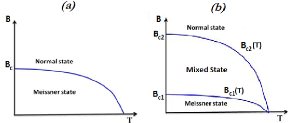
superconductors of Type I: they are in the so-called Meissner state (Fig. 8 (a)). However, their Bc value is limited and for most of their usages they do not work in this

area;

 For magnetic fields between fields Bc1 (lower critical field) and Bc2 (upper critical

field) these materials are in the so-called mixed state (Fig. 8 (b)). In this state, the material as a whole is no longer perfectly diamagnetic and the magnetic flux begins to penetrate inside the material in regions of space that transit to the normal state (called fluxoids): in these conditions the superconducting state and normal state coexist [20].

Fig. 8. Magnetic behaviour of superconductors of Type I (a) and Type II (b). The scale does not represent the real differences between magnetic fields Bc, Bc1 e Bc2

[20].

17

The separation between these two zones takes place due to the spontaneous formation of super-currents, which cause a decay of the field from its maximum value at the center of fluxoid to a zero value in a radius equal to the penetration depth starting to its center. Given that the most part of the material remains in the superconducting state, the material can globally preserve its property of null resistivity even if the field exceeds the field Bc1

(Fig. 9).

Increasing the external magnetic field, the number of fluxoids increases: once the upper critical magnetic field is reached, the material is completely saturated by the field lines that cross it and it can no longer be considered a superconductor.

The value of the upper field Bc2 may reach tens of Tesla, allowing type II superconductors

to be used in the high-field applications.

1.5 Evolution of Superconductors

Since Onnes discovery in 1911, superconductivity has become a fertile ground for researches by the scientific community, which has put great effort driven by the enormous potentials that this phenomenon presents. In recent years, 13 scientists have earned the Nobel Prize for their discoveries in this field.

Regarding to the study of materials, in subsequent decades other superconducting metals, alloys and compounds were discovered with higher and higher performances. Particularly in magnets field, it was crucial the discovery of peculiar Type II superconductor material that can handle great fields and current densities and transit at Tc high enough to reduce

costs and logistical problems.

In 1961, John E. Kunzler identifies a group of superconducting compounds and alloys capable of carrying extremely high currents (106 _A/cm2_{) at high-intensity fields (30 T)}

Fig. 9. Schematic representation of fluxoids and super-currents generated by a transverse magnetic field, which penetrates a type II superconducting material [22].

18

[20]; in 1962, scientists at Westinghouse developed the first commercial superconducting wire, an alloy of niobium and titanium (NbTi), thus starting the studies for superconducting cables for magnets.

NbTi is the first and most used superconducting cable in actual particle accelerators (LHC included); NbTi and Nb3Sn constitute basically the only two materials that are

commercially available for large scale magnet production nowadays. See Fig. 10 for a comparison of their critical surfaces.

NbTi is primarily adopted for its ductility, which allows fabricating it in easier methods: the technique is called “powder in tube” with a synthesis that can be done "ex situ”. At temperature of 4.2 K (liquid helium) its upper critical magnetic field reaches “only” 10 T; cooling with superfluid helium at 2 K increases the field level to about 9 T, as needed in the LHC [23].

Nb3Sn can reach upper critical fields of about 20 T at 4.2 K; this makes it interesting for

developping applications at higher fields. Nb3Sn performance as a function of the

magnetic field are superior compared to NbTi, but there are also some drawbacks. Because of its brittleness, it is not possible to wrap Nb3Sn wires in coils after they are

transited to the superconducting state, in fact, their performance degrades significantly with the mechanical deformation showing an important reduction of their current-carrying capacity. This means that producing a Nb3Sn coil requires special techniques,

such as “wind and react” technique: that impose to all the magnet in its final form to undergo to the thermal processes needed, requiring the utilization of large dimensions furnaces and subjecting all magnet components (supports, insulations etc.) to elevate temperatures for times of hours scale [20].

Then in 1986, Georg Bednorz and Alex Müller obtained the transition of ceramic materials (the family called cuprates) to the superconducting state at temperatures greater than 30 K, pioneering to a new class of superconductors called HTS (High Temperature

Fig. 10. Comparison between the critical surface of NbTi and Nb3Sn [20].

19

Superconductors). Over the years, new HTS materials have been developed, where the most promising are YBCO and BSCCO families, with Tc that can exceed 100 K. See Fig.

11 for a brief evolution of the materials.

These materials can significantly reduce the cost of the cooling system as they can be maintained in the superconducting state without requiring the use of liquid helium or liquid nitrogen, but using liquid hydrogen, which is much less expensive and easier to retrieve. Notwithstanding this, the applicability of such materials remains limited by their cost due to complex manufacturing. By the way, in 2001 it was found the superconducting state of Mg2B2, which has a Tc of 39 K: it has properties of HTS materials but it has a

simple and consolidated method of production.

Fig. 11. Evolution through the years of the superconducting materials based on their critical temperature. Colours indicate the superconductor families [23].

20

CERN

CERN, French acronym for "Conseil européen pour la recherche nucléaire" is an international organization, which manages the world's largest laboratory for studies on particle physics.

The laboratory is located in the northwest area of Geneva on the Franco–Swiss border (Fig. 12).

The agreement among the first 12 member states for the establishment of this organization dates back to September 29, 1954; from this date, the collaboration network has expanded from year to year: today the community counts 22 member states to which must be added several "observer states" from outside Europe. Being a reference point for physics research, CERN also cooperates with a large amount of states around the world.

Many discoveries took place here, the most recently celebrated are the detection of the Higgs boson and discoveries on penta-quarks; numerous awards are won by scientists who conducted experiments here and/or have deduced their theories.

Fig. 12. Aerial view of the CERN area [23].

21

2.1 CERN studies

The heart of the laboratory is constituted by its particle accelerators: the primary purpose of these devices is to investigate many aspects of particle physics; without such means it would be impossible to reproduce certain events in the laboratory and analyse them with an appropriate level of accuracy.

One of the most ample and important investigation concerns the validation of the so-called "Standard Model": the physical theory through which it is possible to describe all the elementary particles of matter and the forces that govern their interactions allowing to understand the fundamental laws that regulate nature; this theoretical model needs experimental verification to validate its predictions. These validations can be carried out only in extreme and strictly controlled conditions, for example, reaching very high levels of kinetic energy of particles, involving high magnetic fields (and thus equally large currents) and working at very low temperatures.

Particle accelerators are fundamental tools to achieve such conditions: they accelerate beams of ions or subatomic particles until they reach the higher possible speed (or accordingly, energy); once the required energies are attained, these beams are collided with each other or with a fixed target.

When two particles having high speed collide with each other a new particle is obtained as a product, which for the well-known law that link mass and energy, E = mc2_{, will have}

an energy, and therefore a mass, greater than the energy of the two particles that generated it. Then, this new particle can decay, giving rise to other particles in precise radioactive cascades; usually because of the rapidity of such decays it is not possible to detect directly the “parent particle", but it is possible to extrapolate its properties from the analysis of the "daughter particles" characteristics. Studying these interactions, theoretical physicists get material to be able to draw important conclusions.

2.2 From larger to smaller

2.2.1 The acceleration chain

When people thinks about devices to accelerate particles used at CERN, the most mentioned it is definitely the LHC (Large Hadron Collider), which with its 27 kilometres in circumference is the largest accelerator in the world. However, this is not the only particle accelerator at CERN and it represents "only" the last stage of the "acceleration chain" that the particles carry out during their life in the laboratory.

The idea is to use accelerators in sequence: a particle beam is initially accelerated in less powerful accelerators and then it is transferred towards ever more powerful accelerators, where it undergoes a gradual increase of energy; the maximum speed, near to the speed of light, are reached at the last stage of this chain: the LHC.

22

The operations that take place inside an accelerator can be divided into three phases [24]:  Injection: during which the beam of particle is prepared by the various pre-accelerators

and injected into the first accelerator of the chain;

 Acceleration: during which the beam is accelerated to the nominal energy of the accelerator;

 Sending or Storage: during which the beam is sent to the next accelerator in the chain or, if it has already been reached the maximum energy required for that specific experiment, this level of energy is maintained for as long as possible and it is made available for physics experiments.

Particle accelerators can be classified according to various principles, one of these is based on their shape from which it depends the number of times that the same particle beam cross it. In linear accelerators particles pass through it only one-time from input to output (they constitute the first stages of the acceleration chain), while in circular accelerators a particle beam travels repeatedly around its loops in order to achieve higher energies.

CERN accelerator system comprises 7 major accelerators to which several experiments are connected [25] (Fig. 13):

 Two linear accelerators that are at the beginning of the acceleration chain: LINAC2: it accelerates protons up to energy of 50 MeV;

LINAC3: it generates heavy ions (usually lead) to 4.2 MeV/nucleon;

 LEIR (Low Energy Ion Ring): circular accelerator where heavy ions produced by LINAC 3 arrive and are then accelerated up to 72 MeV;

 PSB (Proton Synchrotron Booster): circular accelerator consisting of 4 overlapping synchrotrons with a circumference of 50 meters; it accelerates the protons coming from LINAC2 to energy up to 1.4 GeV. It is also used in separate experiments such as ISOLDE;

 PS (Proton Synchrotron): circular accelerator having a circumference of 628.3 meters, it accelerates protons up to 28 GeV; is the most "ancient" accelerator still in operation at CERN;

 SPS (Super Proton Synchrotron): circular accelerator with a 2 km diameter which accelerates protons up to 450 GeV;

 LHC (Large Hadron Collider): circular accelerator having a circumference of 27 km; it accelerates protons up to 6.5 TeV (higher value ever achieved by an accelerator:

23

record obtained in May 2015). For the work presented in this thesis, references will be done to cables used for this accelerator.

The achievement of the highest energies possible is not the principle aim of the acceleration chain. In fact, it can be considered a necessary preparatory step for the following studies (whose quality, however, depends on the acceleration performance), which constitute the “real scope” of the experiment: analyse events of collision between two particle beams traveling in opposite directions and most of all investigate about new particles that result from such impacts. The revelation of particles produced by the impact between beams is a complex and delicate operation as much as that which allows their acceleration.

In LHC two particle beams are made to collide in four points on the accelerator circumference, corresponding to the four main experiments of its scientific program: ATLAS, CMS, LHCb and ALICE (see Fig. 13). Fulcrum of such experiments are huge particle detectors that allow to obtain a great number of information regarding these collision phenomena.

2.2.2 LHC

Fig. 13 CERN accelerators system and experiments [25].

24

In this thesis will be only presented a brief description on the structure of LHC, avoiding details of many components that make up its 27 km length. It will be sufficient to understand its fundamental elements, that allow reaching and maintaining unique conditions in the world.

In LHC, two particle beams are driven from the input speed (at which they arrive from the previous sections of the acceleration chain) up to speed close to the speed of light: the nominal speed is equal to 99.9999991% of its value. At the same time it is crucial that these beams remain confined within the magnet cavities and maintain unaltered their orbit.

To modify the speed (v) and the trajectory of particles (with charge q) electromagnetic fields are used (E, B): they generate a Lorentz force on charges that can be expressed through this formula:

F = q (E + v x B)

A particle undergoes an acceleration in its motion direction due to the electric field E, while the magnetic field B, perpendicular to the velocity vector v, does not vary the kinetic energy of the particle but it is adopted to change its trajectory.

Therefore, it is possible to distinguish two main elements in LHC [25]:

I. Radiofrequency (RF) cavities: through an alternating electrical potential, particles increase their kinetic energy whenever they pass through these elements. It is necessary that the frequency of potential variation is exactly synchronized with the passage of the bunch of particles at every turn, in order to achieve the desired effect (the so-called "kick"). This requires an extremely high level of precision, since the particles pass through each cavity 11245 times per second. In Fig. 14 a model of their structure is shown;

II. Magnets: the 1600 superconducting magnets of LHC can be further divided between:  Dipole Magnets (MB): they generate the magnetic field necessary to keep the two

particle beams traveling in opposite directions in their proper trajectories.

 Quadrupole Magnets (MQ): they generate the magnetic field necessary to focus the particles: beams are composed by electrically charged particles (protons) that naturally tend to diverge from their selves. A single quadrupole is able to focus the beam in just one direction (x or y), defocusing the beam in the other direction at the

Fig. 14. Schematic representation of a radiofrequency cavity [20].

25

same time: in order to get the correct result it is indispensable to couple two quadrupoles which act in directions perpendicular to each other.

 Corrector Magnets: many other high order magnets are placed along the ring to correct the magnetic field errors of the larger main magnets [24].

LHC magnets are organized in 23 regular cells that are repeated along the length of the accelerator (described in Fig. 15), the so-called "FODO cells".

Actual LHC dipoles produce a field equal to 8.3 T, while new high-field magnets that will be soon installed will reach 11-13 T. Note that to reach the actual 8.3 T magnetic fields, a current of 11850 A in the magnet coils is needed. At the same time, studies for even more powerful magnets are carried out. In Table 1 a summary of LHC MB parameters is displayed.

It was mentioned the fact that particles "life" within an accelerator needs to proceed in extremely controlled conditions and it is therefore mandatory to minimize all disturbance

Fig. 15 A schematic layout of a FODO cell (F and D letters are for Focalization in one direction and De-focalization in the other, while O is a space or a deflection magnet): MB are main dipole magnets while MQ are main quadrupoles, the other terms are for corrector magnets [26].

Table 1. Summary of LHC MB main parameters [1].

26

phenomena for detectors. For example, to avoid that particles collides with other gas molecules present in the pipe, thus deviating from their predetermined trajectory, beams flows within a "beam pipe" which is maintained in ultrahigh vacuum conditions. Furthermore, the entire collider and its experiments are placed inside a tunnel at a depth ranging from 50 to 175 meters: this configuration avail to increase the shielding against cosmic radiation that can interact with the particles and alter the experimental results.

2.2.2.1 Why Superconductors?

Having a picture of the quantities involved, is easy to understand why superconductivity has been the most influential technology in the field of accelerators in the last 30 years, preferring these materials than ordinary wires, although the latter have a smaller cost for meter. To get the same results obtained for LHC using ordinary wires, it should require:

 The use of much more normal material.

 The construction of wider and longer tunnels (if normal magnets were used instead of superconducting magnets, the final accelerator would have to be 120 km long to reach the same energy level of LHC) thus having a higher capital cost.

 The installation of a greater power (900 MW of power installed would be needed, equal to the power output of a large nuclear power plant).

 Cope with the huge amount of losses and the removal of the heat produced by Joule effect (normal conductors have higher electrical resistance than superconductors). Consequently, without superconductivity it would not be possible to operate LHC.

2.2.2.2 LHC upgrade projects

High-Luminosity LHC

It is possible to increase performances of an accelerator not only increasing the kinetic energy of particles, but acting on different parameters; luminosity, for example, is extremely important.

Luminosity represents the number of collisions per cross-section, occurring in the unit of time. As in the case of LHC, where collisions happens between particle beams splitted into different bunch of particles, the luminosity is given by:

L = N1· N2 A f

Where N1 e N2 are the number of particles present in the colliding bunches, A is the

average cross-section of the beams and f is the frequency with which two bunches collide.

27

Some of the events that the LHC detectors investigate occur in such a small number during operation, that even long investigation times may not be sufficient to obtain a significant sample of data that can be used as a statistical base for deducing any conclusion.

By increasing the luminosity, it is possible to extend the number of such rare events that are inaccessible at the LHC’s current sensitivity level. For example, after the High-Luminosity implementation, LHC will be able to produce up to 15 million Higgs bosons per year, compared to the 1.2 million produced in 2011 and 2012.

High-Luminosity LHC project aims to increase tenfold the actual luminosity value (bringing it from the value of 1034 _cm−2_s−1 _{to the value of 10}35 _cm−2_s−1_{) for observations}

that will start after 2025.

To perform this upgrade, changes on LHC are planned for the next future; some of them require the overcome of considerable technological step and thus the development of innovative technologies for which many efforts and resources are currently spent. A very important modification involves the replacement of some magnets with a new magnetic system, actually in development. For High-Luminosity LHC project it is necessary the inclusion of additional collimators in the accelerator; that on the other hand, introduce the problem about how to find the space to add new elements within the LHC ring that is already full [25]. To overcome this issue, some of actual dipoles will be replaced with shorter but more powerful magnets, which will be able to reach a magnetic field of 11 T instead of the current 8.3 T [27]. At the same time, 16 new quadrupoles (called MQXF) will be installed in the proximity of the two main experiments to produce magnetic fields greater than the current ones (about 12 T) in order to provide the final beam focusing. It would not be possible to obtain these results using NbTi coils actually in use, therefore it will be necessary to use Nb3Sn for coils, a superconducting material

with higher performance; that material, however, requires the solution of other technological problems, as already introduced in Chapter 1.5.

Very Large Hadron Collider

Why is the size of an accelerator so important? Particles traveling within the accelerator with high energies require a high magnetic field in order to be bended and confined inside the beam pipe; without its effect, particles could bump the accelerator walls and would be lost. As seen for the High-Luminosity project, modifications are performed to increase the magnetic field produced by LHC magnets, however, at the current state of the art it is not feasible to go beyond certain field values. This problem can be solved by increasing the size of the circular accelerator, following this simple rule:

ρ

[m] =

E [GeV]

0.3 q ∙ B [T]

Where ρ is the radius of curvature that a magnetic field B applies on a particle having charge q and an energy E. Once the nature of particles is set (fixing q), it is possible to

28

bend particles of greater energy by increasing the radius (and thus the size) of the accelerator without necessarily increasing its magnetic field.

Hence, in the last years a project has been proposed about the design and build of a new particle accelerator of around 100 km in circumference (VLHC: Very Large Hadron Collider) that exceeds the capabilities of LHC. This project is still under discussion and there is no detailed plan or schedule for the VLHC for the moment.

2.2.3 Magnets

Going deeper inside LHC, it is useful to outline the design of the magnets in order to understand in more detail the technological context in which superconductivity is used.

The superconducting magnets tasks are the bending (dipoles) and the focusing (quadrupoles) of particle beams during their path; note that a magnetic field is able to provide an adequate force only if it is perpendicular to the particle trajectory. To achieve this result, a coil realized with highly compacted superconducting cables, in a characteristic shape called racetrack, is arranged around the beam pipe in which particles flow (Fig. 16). In fact, the magnetic field in a superconducting accelerator magnet is mainly produced by the current in the conductors, rather than the magnetization of an iron yoke [28].

Looking at the section of a magnet as in Fig. 17 (in the case of a dipole, but equivalent can be found into a quadrupole), it is possible to describe the main magnet components. Very schematically, the two beams that travel into the accelerator in clockwise and counterclockwise directions are contained within the same magnet into separated beam pipes in ultrahigh vacuum conditions. Tightly packed superconducting cables are wrapped around pipes to produce the magnetic field. Austenitic steel collars hold the coils in place against the strong magnetic forces that arise when the coils are at full field (the Lorentz forces produced in 1 meter of dipole corresponds at about 400 tons); then an iron yoke sorrounds this assembly closing the magnetic field lines. Electrical bus connection called bus-bars provide the transfer of current between different magnets. Thus, the

Fig. 16. Racetrack configuration for a dipole magnet

29

structure is inserted into a complex cryostatic system: thermal shields and vacuum help to minimize convection and radiation exchanges and, most important, all the system is crossed by superfluid liquid helium at temperature of 1.9 K, which dissipates the input heat by means of heat exchanger tubes, providing cooling to the temperature required for superconductivity. Finally, supports sustain the weight of the magnet: a dipole of a length of 15 meters weighs about 35 tons.

2.2.4 Blocks and windings

In order to generate perfect dipole and quadrupole fields transvers to the beam pipe, it is necessary to obtain current distributions as the ones schematically shown in Fig. 18. In real terms, it is not possible to realize this geometry using a coil, due to the size and rigidity of the cables and the need to use a single long cable around the magnet (joints would create huge losses).

The best approximation of the ideal geometry is obtained by two layers of superconducting cables with rectangular section (with a slight keystone angle), divided

Fig. 17. LHC Dipole cross-section [28].

30

in blocks and separated by copper wedges to give to the coil a circular-like shape [12]. See Fig. 19.

These limitations cause the presence of non-allowed harmonics in magnet bore, which reduce the quality of the resulting field; thus, corrector magnets of highest order are inserted to minimize these field distortions.

The magnetic field obtained with this current density configuration is not constant but variable along the width of the coil, as shown in Fig. 20; anyway, inside the cavity where the field must act properly, it reaches the quality demanded by beam physics requirements.

Fig. 18. Ideal current densities to reproduce perfect dipole (a) and quadrupole (b) fields in the centre of the pipes [20].

Fig. 19. Real configurations of dipole (a) and quadrupole (b) coil geometries used to approximate the ideal ones.

Chapter 2 - CERN

(b)

(a)

31

2.2.5 Rutherford Cables

As explained, superconducting cables have the role of carrying the current needed to produce the required magnetic field. Considering the 27 km of LHC, it may seem that the superconductivity takes place only in a small part of the device (a cable has only few mm2 _{of section); in real terms, the whole length of superconducting cables needs to be}

considered, which is actually extremely long: considering all magnets, superconducting cables of 7600 km long are used, with the characteristics that are described below. “Since the first superconducting accelerator magnets started operation in 1983, only Rutherford type cables are used in the design of all superconducting accelerators” [24]. Rutherford cables are flat cables consisting of multi-filament wires, called strands, arranged to obtain a rectangular section, and then twisted with a specific twist pitch. A twist pitch is the distance after which, looking at the cable main face, one strand returns to its original position. Strands are superconducting filaments formed in turn, by several thousands of micro-filaments of dimensions of few μm (see Fig. 21). The strand fabrication technique is a multi-step process that starts from the insertion of unreacted powder of superconducting material (NbTi, for example) inside a cylindrical matrix of normal material, to favour the phenomenon of current sharing (described in Chapter 3.2.5). As a result of extrusion and swaging processes, the diameter of the micro-filaments is reduced; then, more filaments are coupled together and the process is repeated several times until the number of micro-filaments and the size reach the desired values.

Fig. 20. The magnetic field in one quadrant of LHC dipole magnets with a central field equal to 8.33 T at nominal current. Darker areas represents a higher magnetic field [12].

32

Cable stability increases as the conductor cross-section decreases, for this reason superconductors are made of multi-filament wires with very small dimensions: this help to reduce the flux-jump problem. “This phenomena arises from current induced in the conductor by the presence of a changing magnetic field (for example the magnetic field ramping during charging operations)… These circulating currents extend for a finite length along the conductor, flowing in one direction on one side of the conductor and returning on the other side to complete the circuit” [29]. These currents are superimposed to the transport current, and they can cause a sudden movement of fluxoids, which causes the release of a lot of energy. If the heat generated does not quickly reaches the surface of the filament, in order to be dissipated by the normal material (which has good heat capacity), it can drive an increase of wire temperature that may be irreversible. Reducing the size of the filament allows the reduction of the distance that the heat generated inside the filament has to pass to reach its surface, minimizing the flux jump phenomenon. Unfortunately, this is not sufficient because these coupling currents tend to interact within the cable when two filaments run in parallel; in this case currents create anyway closed paths, passing through the higher resistive normal matrix, causing diamagnetism and unequal distribution of currents in the strands. Twisting filaments (and strands too), forces the flux deriving from the external magnetic field to be alternated through successive short-dimension loops, reducing the effects of the flux jump and allowing a more rapid charge of the magnet.

Moreover, strands are compressed into a flat two layers structure with a trapezoidal shape, slightly keystoned to facilitate the winding into a cylindrical shape around the beam pipe. This configuration allows the highest current densities due to a very high packing factor and their mechanically stable structure [12]. See Fig. 22 to understand the structure. Rutherford cables can differ depending on their use: modifying the geometrical parameters, the number of strands and the materials involved, cables with different properties can be obtained. According to [12], two different types of cables are used inside LHC:

 LHC 01 is utilized for the internal layer of main dipole magnets;

Fig. 21. (a) A cross-section of NbTi filaments. (b) A cross-section of a multi-filament strand. (c) A Rutherford cable. (d) LHC dipole cross-section.

33

 LHC 02 is utilized for the external layer of main dipole magnets and for both layers of main quadrupole magnets;

All LHC cables are built using NbTi. Considering the magnetic field distribution plotted in Fig. 20, it is possible to explain the purpose of different cables within the same magnet: since the field in the outer layer is considerably lower than in inner one, the critical current density that these zones of the winding can support is greater. Thus, it is possible to reduce the superconductor cross-section of cables in the outer layer (LHC 02) hence reducing costs.

The High-Luminosity project, as explained in Chapter 3.2.2.2, requires the replacement of some quadrupoles with more powerful magnets called MQXF; this modification makes it necessary to involve different material for Rutherford cables, such as Nb3Sn, to

substitute NbTi, used nowadays (see Tab. 2 for a comparisons of the main characteristics of NbTi and Nb3Sn cables). Following past studies [1] [1 - 30], this thesis will make

reference at these new Nb3Sn Rutherford cables utilized for MQXF, considering their

geometric parameters.

Fig. 22. (a) Drawing of a Rutherford cable and (b) a real photo.

Table 2. Comparison between High-Luminosity MQXF Nb3Sn cables and actual MQ NbTi cables [1].

Chapter 2 - CERN

34

3.2.5 The current sharing phenomenon

As already mentioned, the reason why the strands that constitutes a superconductive Rutherford cable are designed by coupling superconducting material with normal material is to favour the current sharing: it is useful to describe briefly this phenomenon.

The material can transit even when the temperature does not exceed the Tc, but for

example, when its current density exceeds its critical value Jc. From the definition of

critical surface (see Chapter 1.3) is known that the three parameters involved (T, J, B) are each one a function of the others: setting the magnetic field B as a fixed value, if the temperature increases the critical current density falls. If the field is set, then the current able to generate it is fixed as well. Therefore, it can be expected that an increase in temperature, even very limited, can cause the approaching of current density to its critical value up to its overcoming. In all cases, a transition to the normal state produces an increase in superconductor material resistivity, which it is usually higher than normal materials resistivity. This can generate a relevant amount of heat by Joule effect.

To prevent material damaging due to heat, the superconducting strands are manufactured in composite form: superconducting filaments are immersed in a matrix of copper or another normal metal characterized by a lower resistivity than that of the superconductor in its normal state. In this way, when the temperature exceeds the Tcs value (called current

sharing temperature), the current sharing phenomenon takes place: in the superconducting material flows a current equal to the maximum current density Jc without

being exceeded, while in the normal conductive material flows the remaining current that could not be handled by the superconductor without undergoing transition. Once the temperature surpasses the Tc value, Jc is equal to zero and all current flows in the normal

conductor, realizing a shunt for the superconductor and preventing its damage (see Fig. Fig. 23. Schematic representation of the current sharing phenomenon depending on the evolution of the temperature [20].

Chapter 2 - CERN

35

23 for an operative scheme). This situation can last only for few moments because losses produced in the normal conductor by Joule effect are huge and difficult to handle; therefore, it is fundamental that the system which has to detect and control all sources of heat into the system acts extremely fast.

36

Interstrand coupling currents induced by

time-varying magnetic field

Superconducting cables for accelerator magnets can be subjected to a variety of perturbations involving the release of energy into the system. Not all these disturbances are sources of heat coming directly from outside the system, but in many cases the heat (or better: the losses) originates internally to the cable as a result of phenomena induced by external causes. One of these causes is represented by a magnetic field variable in time.

In LHC, during operations of injection of particles and of beam dump at the end of the survey period, the magnetic field is ramped up or down at speeds that vary according to the needs, thus creating magnetic field cycles variable in time, that repeat several times during the life of a magnet.

A variation of the magnetic field induces an electromotive force (

ε

) on a conductor loop (superconductive or not), which corresponds to an electric field that forces the charges to flow around the wire: thus, currents are induced inside the conductor. According to the Faraday’s law, the induced electromotive force in a coil (thus the intensity of the induce currents) is proportional to the opposite of the rate of change of magnetic flux ΦB:

ε

=

-

dΦB dt

For this study, only variations in B (the field normal to the cable main face) will be considered, since the magnitude of the induced eddy currents is mainly affected by this component.

In a Rutherford cable, these currents can be induced on more "levels": in fact, intrastrands (or interfilament) eddy currents and interstrand eddy currents coexist. The first ones originates at the level of filaments that constitute strands, mostly in the normal resistive matrix that surrounds the individual superconducting filaments (introduced to reduce the problem of the flux-jump). The second ones flow and connect the various strands that compose the cable. It is possible to study these current distributions separately in consequence of their different time constants [7]. This thesis is focused on the latter, which are here described.

Interstrand eddy currents can be distinguished between:  Interstrand Coupling Currents (also called ISCCs [2])

37

They circulate between the various strands creating loops, which close flowing through the points of contact between strands. Their form depends on the particular geometry of Rutherford cables (several strands twisted and not isolated with each other). Depending on the position of one strand over another, they can circulate around two different paths [32]:

 Diamond-shaped loops, which connects one strand of the upper layer and one of the lower layer, by cross-over points of contact characterised by a resistance Rc.  Parallel-strand loops in which the current flows between adjacent strands and

where contact points are characterized by a resistance Ra.

It is possible to refer at Ra and Rc together, calling them ICRs (interstrand contact resistances); see a representation of ICRs and current loops on a cable in Fig. 24 – 25 - 26. The greater is the area of the loop and the higher is the intensity of the current flowing in it; twisting strand can be useful to reduce these areas.

Fig. 25. 3D representation of a Rutherford cable with 10 strands, with the highlight of a typical current loop induced by a normal magnetic field variation in a cable. Adjacent resistances Ra are displayed in yellow and cross-over resistances Rc in red [33].

Chapter 3 -Interstrand coupling currents induced by time-varying magnetic field

Fig. 24. Rutherford cable with the highlight of a typical current loop induced by a normal magnetic field variation in a cable [31].

38

These currents exhibit time constants of typically 0.01 to 10 seconds and have a characteristic loop length of one twist pitch [2]. For this reason, they are also referred as short-range coupling currents.

The model presented on this thesis focuses on ISCCs distribution.

 Boundary-induced coupling currents (also called BICCs or “supercurrents” [2]) They are caused by inhomogeneities (intended as "boundaries" between two areas with different characteristics, hence their name) along the length of the cable, such as magnetic field B or ICRs (i.e. at joints, coil ends, or for manufacturing errors etc.). BICCs differ from ISCCs because they flow into strands over distances of 10-103 _{times the cable pitch, for this reason they are also referred as long-range coupling}

currents.

Following the scheme of Fig. 27, in a cable consisting of only 2 strands, a magnetic field variable in time and space is applied. On the right of the point z = 0, the cable is subjected to a field variation dB/dt that induces ISCCs circulating in each loop at z > 0, while on the left of the point z = 0, the field is constant and at the initial time no current is induced. “However, the current in circuit 5 generates a voltage in circuit 4 which has to be compensated for since dB/dt = 0 in circuit 4. This is achieved by an additional current with alternating direction being generated in all contacts. This results finally in a large current loop where one strand carries positive current and the other negative current” [2]: these are the BICCs.

Fig. 26. Schematic representation of a portion of the cable length with resistances Rc and Ra represented as lumped parameters.

Chapter 3 -Interstrand coupling currents induced by time-varying magnetic field

39

They exhibit large characteristic times of 102 _{÷ 10}5 _{s (for practical cables) which are}

several orders of magnitude larger than the time constant of the interstrand coupling currents [2]. Furthermore, their amplitude can be orders of magnitude higher than short-range coupling currents [7], and it increases strongly if the lengths of the B variations are of the same order or smaller than the cable twist pitch.

Despite the intensity of these currents is generally not high, BICCs and ISCCs are the source of several problems:

 They compete with the transport current reducing the Ic, thus affecting the cable

stability [2].

 Even when they are too weak to cause reductions of Ic, they are responsible for the

so-called “dynamic magnetization” that induces multipolar harmonics in the dipole and quadrupole bore field, causing their distortion [34].

 They cause the introduction of power in the system. For ISCCs, the current flowing from one strand to another pass through ICRs dissipating heat, while BICCs “stay in the strands and that implies that they generate almost no heat compared to the inter-strands coupling losses” [3]. To ensure the stability of a magnet, it is very important to estimate the value of these losses; the aim of this thesis is precisely to analyse their magnitude and distribution in cables and how they change varying several parameters.

Since operation of field ramping cannot be avoided, a way to reduce ISCCs and BICCs and the corresponding losses is to act on resistances Rc and Ra, ensuring that they are kept within certain "compromise ranges". These resistances should be sufficiently high in order to suppress or reduce the coupling currents, but still enough low to guarantee a proper current sharing between strands and not affect stability [14 - 15]. In Chapter 5 a methodology to work in this direction is introduced and discussed.

Since the term stability has already been introduced, it may be useful to explain it briefly: despite not pertaining to the objectives of this thesis it is related the importance of calculation of losses due to electrodynamic transient.

Fig. 27. Representation of ISCCs and BICCs generated in a 2 strands cable due to magnetic field varying in time and space [2].