Brain vasculature segmentation for SEEG pre-operative planning via adversarial neural network approach

(1)

POLITECNICO DI MILANO

Dipartimento di Elettronica, Informazione e Bioingegneria

Laurea Magistrale in Biomedical Engineering

Brain vasculature segmentation

for SEEG pre-operative planning

via Adversarial Neural Network approach

Supervisor: Prof.ssa Elena De Momi

Dott. Francesco Cardinale

Co-Supervisor: Dott.ssa Sara El Hadji

Author: Tommaso Ciceri

Student ID: 899621

(2)

(3)

i

Sommario

La segmentazione dell’albero cerebrovascolare ricopre un ruolo fondamentale nella neurochirurgia in ambito pre- e intra- operativo. In particolare, scenari come la StereoElettroEncefaloGrafia (SEEG), tecnica di registrazione basata sull'impianto percutaneo di elettrodi intracerebrali per l’identificazione della zona epilettogena (EZ) responsabile delle crisi epilettiche focali, richiedono una visualizzazione accurata dell'albero vascolare per la pianificazione e l'esecuzione dell'intervento. Tradizionalmente, è il neurochirurgo che, attraverso la sua esperienza e conoscenza, pianifica l’intervento di SEEG. In primo luogo osserva ed analizza diverse tipologie di immagini e successivamente seleziona manualmente i punti di ingresso ed i punti di destinazione degli elettrodi intracerebrali. Tuttavia questa fase di pianificazione dell’intervento risulta stressante e dispendiosa, poiché sono richieste circa 2-3 ore di lavoro per l’intera procedura.

In questo lavoro di tesi ci siamo focalizzati nel cercare di automatizzare gli step svolti dal neurochirurgo per segmentare i vasi cerebrali, cercando di ridurre il tempo richiesto di pianificazione della segmentazione vascolare (da ~ 30 minuti ad 1 minuto), la sua dipendenza dall’operatore ed i tipi di immagini necessarie per generare l’immagine segmentata, evitando così una dose eccessiva di raggi X somministrata al paziente ed i relativi errori di co-registrazione delle immagini. In particolare, dell’attuale flusso di lavoro per la segmentazione dei vasi cerebrali svolto nel Centro Chirurgia dell’Epilessia “Claudio Munari” all’ospedale Niguarda di Milano, che richiede l’acquisizione di minimo due diverse tipologie di immagini, vogliamo automatizzare i seguenti passaggi: co-registrazione di diverse immagini, somma e sottrazione di immagini e thresholding manuale finale. A tal fine abbiamo implementato e confrontato diversi metodi per la segmentazione automatica dei vasi cerebrali.

Abbiamo utilizzato un dataset anonimizzato relativo a 50 pazienti fornito dal Centro Chirurgia dell’Epilessia “Claudio Munari” dell’ospedale Niguarda di Milano, composto da due differenti tipi di volumi di Cone-Beam Computed Tomography (CBCT) acquisiti precedentemente e successivamente all’iniezione del mezzo di contrasto. Da essi è stato possibile ricostruire un’angiografia a sottrazione digitale (DSA) che, una volta binarizzata, ci ha permesso di ottenere la nostra maschera finale di segmentazione dei vasi usata come riferimento, gold standard.

(4)

ii

Abbiamo utilizzato questo dataset per investigare diverse architetture per la segmentazione di vasi, ed in particolare, ci siamo focalizzati sull’implementazione di reti innovative Adversarial Neural Network (ANN), sia in una versione 2D che 3D, che ci hanno permesso di combinare il potenziale di segmentazione delle Fully Convolutional Neural Network (FCNN), con la capacità discriminatoria delle Generative Adversarial Network (GAN). L’architettura da noi proposta è stata confrontata con alcune FCNNs e con uno dei metodi di riferimento più noti e utilizzato in letteratura per la segmentazione di vasi, ovvero Frangi filter. Le FCNNs che abbiamo preso in considerazione sono la U-net, una delle più note reti neurali usata per la segmentazioni di immagini mediche, e alcune sue varianti (Residual U-net, MultiResU-net, Nested U-net).

I risultati presentati in questo lavoro hanno evidenziato che le ANNs hanno una migliore capacità di segmentazione in termini di Dice Similarity Coefficient (DSC) rispetto alle FCNN ed al Frangi filter. Infatti, con la migliore ANN implementata, la sua versione 3D, abbiamo ottenuto un valore mediano di Dice Similarity Coefficient (DSC) pari a 85.8%, con un intervallo interquartile (IQR) del 19.9%; contro un valore mediano di DSC del 79.9% con un IQR del 30.1% ottenuto con la migliore FCNN e un valore mediano di DSC di 60.2% con IQR pari a 9.2% ottenuto con l’applicazione del metodo riferimento (Frangi filter). Confrontando le distribuzioni di DSC ottenute nei tre casi sopracitati le ANN si sono rilevate significativamente migliori rispetto agli altri metodi (p-value < 0.05, Kruskal-Wallis test).

Da questo lavoro si può evincere che un approccio basato sul deep learning, ed in particolare su reti neurali avversarie, fornirebbe al neurochirurgo un modo alternativo e meno dispendioso - il tempo da dedicare ad ogni singolo paziente scenderebbe sotto al minuto - per segmentare i vasi cerebrali rispetto al metodo attualmente utilizzato. In particolare, considerando il flusso di lavoro svolto per la segmentazione dei vasi cerebrali dal Centro Chirurgia dell’Epilessia “Claudio Munari”, con questo nuovo approccio sarebbe possibile evitare i passaggi intermedi quali la co-registrazione di diverse immagini, somma e sottrazione di immagini ed il thresholding manuale, inevitabilmente soggetto ad arbitrarie ed individuali interpretazioni. Inoltre una volta allenata la nostra rete neurale, per segmentare nuove immagini di vasi cerebrali sarà necessario soltanto avere il volume CBCT acquisito dopo l’iniezione del mezzo di contrasto. In questo modo, l’acquisizione dei volumi di CBCT prima dell’inserimento del mezzo di contrasto è evitata, in quanto non più necessaria per lo

(5)

iii

scopo finale di segmentazione cerebrovascolare, riducendo la dose di raggi X somministrata al paziente.

(6)

iv

Summary

The segmentation of the cerebrovascular tree plays a fundamental role in pre- and intraoperative neurosurgery. In particular, scenarios such as StereoElectroEncephaloGraphy (SEEG), a registration technique based on the percutaneous implantation of intracerebral electrodes to identify the epileptogenic zone (EZ) responsible for focal epileptic seizures, require an accurate visualization of the vascular tree for the planning and the carrying out of the surgery. Traditionally, it is the neurosurgeon who, through his experience and knowledge, plans the SEEG intervention. First, he observes and analyzes different typologies of images and, then manually, he selects the entry and destination points of the intracerebral electrodes. However, this planning phase is stressful and expensive, as it requires around 2-3 hour of work for the entire procedure.

In this thesis work, we focused on trying to automate the steps taken by the neurosurgeon to segment the brain vessels, attempting at reducing the time required to plan the vascular segmentation (from about 30 minutes to 1 minute), its dependence upon the operator and the types of images needed to generate the segmented image, thus avoiding an excessive dose of X-rays administered to the patient and the corresponding image co-registration errors. In particular, of the current workflow for brain vessel segmentation carried out in the Epilepsy Surgery center “Claudio Munari” at Niguarda Hospital in Milan, that requires the acquisitions of at least two different types of image, we want to automate the following steps: co-registration of different images, summation and subtraction of images and final manual thresholding. To this end, we have implemented and compared different methods for the automatic segmentation of brain vessels.

We collected an anonymized dataset of 50 patients from the “Claudio Munari” center for Epilepsy and Parkinson Surgery at Niguarda Ca’ Granda Hospital of Milan (Italy), composed of two different types of Cone-Beam Computed Tomography (CBCT) volumes, which are acquired before and after the contrast medium injection. From them, it was possible to obtain the digital subtraction angiography (DSA), then once binarized, it allowed for the generation of the final ground truth vessel segmentation, used as a reference mask.

Several architectures for vessel segmentation have been investigated using this dataset, and in particular, we have focused on the implementation of innovative Adversarial Neural Networks (ANN), both in 2D and 3D versions, which have allowed us to combine

(7)

v

the segmentation ability of Fully Convolutional Neural Networks (FCNN), with the discriminatory capacity of Generative Adversarial Networks (GAN). Our architecture has been compared with some FCNN and with the reference method used in literature for the segmentation of vessels, Frangi filter. The FCNNs we have taken into consideration are the U-net, the most well-known neural networks used for the segmentation of medical images, and its variants (Residual U-net, MultiResU-net, Nested U-net).

The results presented in this dissertation highlighted that ANNs have a better segmentation ability in terms of Dice Similarity Coefficient (DSC) compared to FCNN and Frangi filter. In fact, considering the best implemented ANN, its 3D version, we achieved a median value of Dice Similarity Coefficient (DSC) equal to 85.8%, with an interquartile range (IQR) of 19.9%, against a median value of DSC of 79.9% with an IQR of 30.1% obtained with the best FCNN and a median value of DSC of 60.2% with IQR equal to 9.2% obtained with the application of the reference method (Frangi filter). Comparing the DSC distributions obtained in the three above mentioned cases, the ANN proved to be significantly better than the other methods (p-value < 0.05, Kruskal-Wallis test).

From this study, we can conclude that a deep learning approach and, in particular, an adversarial neural network architecture, would provide the neurosurgeon with an alternative and less stressful way to segment the brain vasculature with respect to the current method (less than 1 minute per patient). In particular, considering the workflow applied by the “Claudio Munari” center for Epilepsy and Parkinson Surgery to segment the brain vasculature, intermediate steps like image co-registration, summation, subtraction, and manual thresholding that is, inevitably subject to arbitrary and individual interpretations, will be automatically exploited by the proposed Neural Network architecture. Furthermore, once our neural network has been trained, it will only be necessary to have the CBCT volume acquired after the injection of the contrast medium to segment new images of brain vessels. In this way, the acquisition of CBCT volumes before contrast medium injection is avoided, as it is no longer necessary for the final purpose of cerebrovascular segmentation, thus reducing the X-ray dose administered to the patient.

(8)

vi

List of Figure

Figure 1.1.1: Brain activity with and without an epileptic seizure. ... 2

Figure 1.1.2: Workflow applied to patients before undergoing surgery treatment after the failure of the antiepileptic medications. ... 4

Figure 1.2.1: Fundamental steps of the postprocessing workflow to segment the brain vasculature. ... 5

Figure 1.2.2: DSA image representation. ... 6

Figure 1.3.1: Comparison between the proposed approach and the current pipeline. ... 8

Figure 2.1.1: Segmentation results near the left posterior communicating artery ... 14

Figure 2.1.2: Segmentation results for small and large vessels. ... 15

Figure 2.1.3: Comparison of anterior and lateral views of MIP images derived from 3D rotational angiography (A) and 3D Deep Learning Angiography (B) datasets of a patient evaluated for posterior cerebral circulation. ... 16

Figure 3.1.1: Workflow of the tested approaches for brain vascular segmentation. ... 19

Figure 3.1.2: Pre-processing workflow to obtain the binary segmentation of the Digital subtraction angiography (DSA) volumes. ... 21

Figure 3.1.3: Standard or Enhanced acquisition protocol. ... 22

Figure 3.1.4: Workflow comparison between the standard surgical procedure and the O-arm system procedure. ... 23

Figure 3.1.5: CT cone-beam acquisition geometries. ... 23

Figure 3.1.6: Result of a DSA volume manually thresholded. ... 25

Figure 3.1.7: 2D datasets. ... 27

Figure 3.2.1: FCNN wiring exploiting spatially‐local correlation. ... 29

Figure 3.2.2: Multiple features maps into a single layer. ... 30

Figure 3.2.3: Example of max pooling layer application. ... 31

Figure 3.2.4: Example of up-sampling and transpose convolutional layer application. ... 31

Figure 3.2.5: Activation function representation of the Rectified Linear Unit layer. ... 32

Figure 3.2.6: Scheme of Ronneberger et al. U-net architecture ... 34

Figure 3.2.7: Scheme of the identity block. ... 36

Figure 3.2.8: Scheme of the convolutional block. ... 36

(11)

ix

Figure 3.2.10: MultiRes block proposed by Ibtehaz et al. ... 39

Figure 3.2.11: Example of Res path connection proposed by Ibtehaz et al. ... 39

Figure 3.2.12: MultiResU-net architecture. ... 40

Figure 3.2.13: Scheme of W-net proposed implementation. ... 42

Figure 3.3.1: GAN architecture. ... 49

Figure 3.3.2: Scheme of SegAN generator proposed implementation. ... 51

Figure 3.3.3: Scheme of SegAN proposed implementation. ... 53

Figure 3.4.1: Confusion matrix. ... 58

Figure 4.1.1: Graphical representation of the Dice similarity coefficient (DSC) median 2D 1-channel vs 2D 3-channel testing phase results of all the FCNNs proposed. ... 62

Figure 4.1.2: Graphically representation of the DSC median patches testing phase results of all the FCNNs proposed. ... 64

Figure 4.1.3: Graphical representation of the IQR patches testing phase results of all the FCNNs proposed. ... 64

Figure 4.3.1: Boxplots of the Dice similarity coefficient (DSC) median segmentation performance metric obtain with the SegAN Generator (FCNN reference architecture), 3D SegAN architecture (ANN proposed architecture), and Frangi filter (state of the art approach). ... 68

Figure 5.2.1: Comparisons between the slices extracted from the original (Cone Enhanced-Cone Beam Computed Tomography, CE-CBCT) volume, the ground truth, the 3D SegAN predicted volume and the comparison between the ground truth and the 3D SegAN prediction. ... 72

Figure 5.2.2: Comparisons between the slices extracted from the original (Contrast Enhanced-Cone Beam Computed Tomography, CE-CBCT) volume, the Digital subtraction angiography (DSA) volume, the ground truth volume, and from the 3D SegAN predicted volume... 73

Figure 5.2.3: 3D rendering of one patient’s Digital Subtraction Angiography volume. ... 74

Figure 5.2.4: Comparisons between the Fully convolutional neural network (FCNN) reference architecture, the adversarial neural network (ANN) proposed architecture and the state of the art approach (Frangi filter). ... 75

(12)

x

List of Table

Table 3.1.1: Number of patients used for the training, validation, and testing set. ... 20 Table 3.1.2: Summary of the training, validation and testing datasets generated. ... 28 Table 4.1.1: Median (interquartile range (IQR)) of performance metrics for different FCNNs

trained on the 2D 1-channel dataset and on the 2D 3-channels dataset. ... 61 Table 4.1.2: Median (interquartile range (IQR)) of performance metrics for different FCNNs

trained on the 2D 1-channel dataset and on the two 2D 1-channel patches dataset (256x256 pixels dataset and 128x128 pixels dataset). ... 63 Table 4.1.3: Median (interquartile range (IQR)) of performance metrics for the original

SegAN Generator (characterized by 9 stages) compared to its sub-networks (characterized by 7 and 5 stages). ... 66 Table 4.2.1: Median (interquartile range (IQR)) of performance metrics for the 2D SegAN

and the 3D SegAN trained on the 2D 1-channel 256x256 patches dataset and on the 3D dataset, respectively. . ... 67 Table 4.3.1: Median (interquartile range (IQR)) of performance metrics for the SeGAN

Generator, the 2D SegAN, the 3D SegAN, and the Frangi’s 3D multi-scale vesselness filter. ... 68

(13)

xi

Abbreviations

ANN: Adversarial Neural Networks BCE: Binary Cross Entropy

BM: Bone Mask

BN: Batch Normalization

CBCT: Cone Beam Computed Tomography

CE-CBCT: Contrast Enhanced Cone Beam Computed Tomography CM: Contrast Medium

CNN: Convolutional Neural Network

FCNN: Fully Convolutional Neural Network CT: Computed Tomography

DICOM: Digital Imaging and Communications in Medicine DL: Deep Learning

DSA: Digital Subtraction Angiography DSC: Dice Similarity Coefficient EZ: Epileptogenic Zone

FFNN: Feed-Forward Neural Network FN: False Negatives

FP: False Positives

GAN: Generative Adversarial Network GPU: Graphical Interface Unit

GT: Ground Truth

ICA: Internal Carotid Artery IQR: InterQuartile Range LA: Learning Algorithm MAE: Mean Absolute Error

MIP: Maximum Intensity Projection ML: Machine Learning

MRA: Magnetic Resonance Angiography MRI: Magnetic Resonance Imaging MS: Multi-Scale

(14)

xii

NIfTI: Neuroimaging Informatics Technology Initiative ReLU: Rectifying Linear Unit

ResNet: Residual Neural Network SEEG: StereoElectroEncephaloGraphy SegAN: Segmentation Adversarial Network SGD: Stochastic Gradient Descent

TN: True Negatives TOF: Time-Of-Flight TP: True Positives VA: Vertebral artery

(15)

1

CHAPTER 1

INTRODUCTION

The goal of this Chapter is to give an insight into the general framework in which this thesis work is inserted. In Section 1.1 epilepsy disease, its current therapeutic approach and the SEEG pre-operative procedure planning for patients that undergo surgical treatment are introduced. In Section 1.2 the processing steps to process the brain vasculature used for SEEG procedure at the “Claudio Munari” center for Epilepsy and Parkinson Surgery, Niguarda Ca’ Granda Hospital of Milan (Italy), are overviewed, underlying current critical issues in this scenario.

Finally, in Section 1.3 the main contributions of this work are discussed.

Epilepsy is one of the most common neurological diseases that affects approximately 50 million people worldwide [1].

Epilepsy is defined by the International League against Epilepsy as “a transient occurrence of signs and/or symptoms due to abnormal excessive or synchronous neuronal activity in the brain” [2]. In fact, in pathological conditions, the brain electric activity is non-synchronous; this ensures that the signal travels through the brain. Meanwhile, during an epileptic seizure, there is an abnormal burst of neurons firing off electrical impulses. These abnormal events disrupt the nerve cell activity in the brain and the body, that start behaving strangely.

In order to diagnose epilepsy, at least two unprovoked epileptic seizures are generally required. Besides, symptoms of epilepsy, such as temporary confusion, loss of consciousness, staring into blank space, uncontrollable twitching of the arms and legs, differ depending on the type of seizure. After the diagnosis, epileptic seizures are classified by clinicians as either focal or generalized, depending on how the abnormal brain activity

(16)

2

begins. In particular, in the focal epileptic seizure, only a part of the brain is affected by abnormal spiking activity, whereas in the generalized epileptic seizure all areas of the brain are affected (Figure 1.1.1) [3].

Figure 1.1.1: Brain activity with and without an epileptic seizure. Brain activity in absence of the seizure on the top; brain activity affected by an epileptic seizure focalized in the middle, and generalized in the bottom of the figure. Adapted from [4].

Epilepsy can be treated with antiepileptic drugs or, for patients suffering from focal epileptic seizures, surgically. Clinicians assert that some habits such as having a proper diet, sleeping, staying away from illegal drugs and alcohol can reduce the possibility of triggering seizures in individuals suffering from epilepsy [5]. There is not a known and efficient method to prevent epilepsy because the treatment gap is enormous, especially in low and middle income countries where antiepileptic drugs are inaccessible or too expensive [6], [7]. Furthermore, nearly 60% of people affected by epileptic seizures suffer from focal epileptic seizures, and 25% of them are medically refractory to antiepileptic drug treatments [8], [9]. This dissertation focuses on patients who receive surgical treatment, which counts around 7 million people worldwide. For drug resistant patients, the goal of the surgery is the resection or disconnection of the epileptogenic zone, defined as “site of the beginning and primary organization of the epileptic seizures” [10]. To apply the resection procedure is necessary to individuate the epileptogenic zone. In 25% to 50% of subjects, identification of the epileptogenic zone requires the use of intracranial electroencephalography recordings [11].

(17)

3

This recording can be done with a cortical grid or with an image-guided technique called StereoElectroEncephaloGraphy (SEEG). The electroencephalography with a cortical grid allows for the recording of the cortical activity of the brain only, and it is the most invasive and risky procedure. In particular, this technique requires the placement of a large array of electrodes called “subdural grid” on the surface of the brain [12]. To expose the brain's surface, patients need to undergo a larger surgery called craniotomy. In contrast to intracranial electrode studies with a cortical grid, the SEEG is a minimally invasive image-guided surgical procedure that consists of placing several multi-lead intracerebral electrodes for a three-dimensional (3D) investigation aimed at localizing the epileptogenic zone.

SEEG has been developed by Bancaud and Talairach at Hôpital Sainte Anne, Paris, France in the late 1950s [10]. Traditional Talairach methodology [13] includes two surgical steps: stereotactic angiography and electrode implantation. This workflow was updated toward a 1-step surgical technique.

SEEG pre-operative procedure planning can be divided into two major steps (Figure 1.1.2): 1. images fusion: acquisition and processing of all biomedical images needed, in order

to obtain denoised brain image with brain vasculature enhanced. In particular, in these steps, despite the several improvements in technologies and new approaches, the vessel segmentation remains challenging. Indeed, the intricate and dense structures of vessels complicate the identification of the best method for this purpose; 2. electrodes trajectories planning: planning of electrodes trajectories through collected images, taking into account various constraints such as avoid blood vessels, sulci, and trajectories crossing.

The SEEG pre-operative planning procedure is performed by a neurosurgeon and it is the most important step for minimizing the risk of complications during surgery such as bleeding, infections, cerebrospinal fluid leakage and, in the worst case, serious injuries or even death [14].

(18)

4

Figure 1.1.2: Workflow applied to patients before undergoing surgery treatment after the failure of the antiepileptic medications. EZ indicates the epileptic zone that has to be localized before surgery. In particular, the SEEG pre-operative workflow can be divided into two steps: image fusion and, planning electrodes trajectories.

Until the early 2000s, the brain vasculature was only enhanced with stereotactic angiography, the first surgical step of the Talairach methodology, as introduced in Section 1.1. The stereotactic angiography was performed in a stereotactic coordinate system through catheter angiography in which a catheter was inserted into an artery through a small incision in the skin to inject the Contrast Medium (CM). All the experienced SEEG centers (e.g., “Claudio Munari” center for Epilepsy and Parkinson Surgery) followed this Talairach’s step as a gold standard for vessel enhancing purposes. With the advent of new non-invasive modalities as Time-of-Flight angio-MR, Phase-Contrast angio-MR, gadolinium-enhanced angio-MR, and angio-CT, many centers started to update their workflow combining different imaging techniques to improve the outcome accuracy[15].

Since Fall 2009, the “Claudio Munari” centre for Epilepsy and Parkinson Surgery updated its vessel enhancing workflow, obtaining a final vessel vasculature segmentation with a 3D Digital Subtraction Angiography (DSA) [13] technique. The processing pipeline to obtain the DSA is described hereafter (Figure 1.2.1):

a) after the catheter insertion, the neurosurgeon proceeds with the first acquisition of the so-called Bone Mask (BM), which is composed of bone and soft tissues;

(19)

5

b) subsequently, the contrast medium is injected and the procedure moves on to the second acquisition, which aims at capturing cerebral vasculature, besides the remaining information (bone, soft tissues);

c) the dataset obtained during selective CM injection in the Internal Carotid Artery (ICA) is chosen as a reference dataset. Optional datasets with CM injection in the contralateral ICA and/or vertebral artery (VA) are obtained when needed;

d) the BM, as well as the optional datasets, is automatically registered to the reference dataset. The registrations are performed with FLIRT, the tool for linear registrations provided by FSL;

e) all vascular datasets are summed to produce a unique dataset, and the bone mask is subtracted obtaining the DSA;

f) manual thresholding based only on visual guidance of the DSA volume.

Figure 1.2.1: Fundamental steps of the postprocessing workflow to segment the brain vasculature. In particular, the Bone Mask (BM), the Left Internal Carotid Artery (ICA) and the Vertebral Artery (VA) volumes are registered with respect to the Right ICA volumes. Then all the vascular datasets are summed to produce a unique dataset, and the registered bone mask is subtracted obtaining, after the thresholding step, the digital subtraction angiography (DSA).

Despite this new method allows for an optimal rendering result of the vascular tree for image guidance during epilepsy surgery [16], it is a complex multi-step process that requires the implementation of many intermediate processing steps on the original image by the operator (such as co-registration, summation, subtraction, and thresholding), and that takes about 30 min. This need for some operator-dependent steps could be a source of error, introducing

(20)

6

variation on the final results. Furthermore, this method presents some drawbacks concerning the image acquisition process, that will be described in detail in Section 3.1.1, and the processing pipeline.

The main problems in the acquisition process are:

• patient motion artifacts caused by the misregistration between the different dataset acquisition procedures. The final result of these artifacts is represented in Figure 1.2.2, which is a DSA before the application of manual thresholding, where are still present structures like mandible, nose, and eyeballs despite it should contain only vessels;

• patients undergo at least double X-ray radiation dose due to the necessary acquisition of two different datasets before and after the injection of the CM. This dose could increase if other optional datasets are requested.

Figure 1.2.2: DSA image representation. The DSA is obtained after the summation of all the vascular datasets, followed by the subtraction of the BM volumes. It is possible to notice the presence of the vessel, the mandible (green arrow), nose (orange arrow), and the eyeball (blue arrow).

On the other hand, the main problems concerning the processing pipeline are related to its thresholding step, which is a process:

• user-dependent;

(21)

7

• that could lead to noisy results or too thin vessel.

Given the possible challenges, the neurosurgeon does not completely rely on this pipeline and verifies that each automatically calculated trajectory that takes into account vascular segmentation does not cross any vessel. This double-check, in some cases, led the neurosurgeon to re-plan the optimal trajectory as the one proposed by the automatic planner did not comply with the requirements of safety distance from the vessels.

Starting from the clinical challenges that neurosurgeons have to overcome before and during the SEEG procedure, the most demanding one is to avoid intracerebral hemorrhage in the patient. In fact, no quantitative information is provided to neurosurgeons regarding the effective position of the vessels in the brain during the surgery, but only qualitative information in terms of brain vasculature angiography.

This work aims at proposing a novel accurate automatic method for the segmentation of brain vascular structure based on a Deep Learning (DL) approach, and in particular via an Adversarial Neural Network (ANN) in a 3D version. The proposed one-step method is intended to substitute a wider image-processing pipeline used for the pre-operative planning of SEEG vessel segmentation procedure currently used at “Claudio Munari” center for Epilepsy and Parkinson Surgery, Niguarda Ca' Granda Hospital in Milan. Intermediate steps like image co-registration, summation, subtraction, and thresholding necessary to obtain the final DSA, will be completely replaced by the proposed Neural Network architecture (Figure 1.3.1), thus minimizing the requested vessel segmentation time and the user-dependency. Furthermore, since only the 3D cerebral angiograms need to be acquired with the proposed method, the radiation dose administered to the patients will be reduced and with it the misregistration problems.

This work involved an anonymized dataset provided by “Claudio Munari” center for Epilepsy and Parkinson Surgery acquired with O-arm System from 2017.

In detail, we are going to investigate the following aspects:

• the implementation and application of different existing FCNN architectures to the segmentation problem considered:

(22)

8

o different connections between layers, e.g., skip and residual connections; • the investigation of specific training aspects which are considered critical for the task

here addressed:

o amount, resolution and level of information provided to the network during the training process;

o cost function employed to train the network;

• the implementation and adaptation of an innovative ANNs for brain vasculature segmentation, in a 2D and 3D version.

Figure 1.3.1: Comparison between the proposed approach and the current pipeline. The proposed method is intended to substitute the image-processing steps (such as image co-registration, summation, subtraction, and manual thresholding), necessary to obtain the final binary vessel segmentation mask, with a 3D Adversarial Neural Network.

This project is developed in collaboration with the “Claudio Munari” center for Epilepsy and Parkinson Surgery, Niguarda Ca’ Granda Hospital, one of the main centers in Italy for SEEG surgical treatment.

(23)

9

CHAPTER 2

LITERATURE REVIEW

Blood vessel segmentation is a crucial topic in the field of medical image analysis since the analysis of vessels is fundamental for diagnosis, treatment planning and execution, and evaluation of clinical outcomes.

Blood vessel segmentation could be achieved through manual or semi/automatic methods. Manual methods are expensive procedure in terms of time and lacking in terms of intra- and inter-operator repeatability and reproducibility. On the other hand, semi-automatic or automatic methods require at least one expert clinician to interact or to evaluate the obtained segmentation result. However, semi-automatic or automatic methods can play a role of assistance for the clinicians in performing their operative tasks.

In this Chapter, the most recent and innovative semi-automatic and automatic vessel segmentation techniques will be presented in Section 2.1, focusing in particular on SEEG methods in Section 2.2.

The cerebrovascular tree is composed of arteries and veins appearing as elongated features with a complicate profile model due to their cross and branch structures. Signal noise, drift in image intensity and lack of image contrast are significant challenges to overcome for the extraction of detailed blood vessels morphology information [17].

Vessel segmentation approaches can be classified into four different categories [18]: • vessel enhancement;

• deformable models; • tracking;

(24)

10

Through vessel enhancement approaches, the quality of the vessel perception is improved, e.g., by increasing the vessel contrast with respect to background and other non-informative structures. Several enhancement methods exist such as matched filtering [19], vesselness-based approaches such as Frangi et al.’s filter [20], Wavelet [21] and diffusion filtering [22]. In detail, the Frangi filter is a vessel detection filter based on Hessian eigenvalues based approach. A vessel detection filter based on Hessian can be described as:

𝐹(𝑥) = 𝑚𝑎𝑥_𝜎𝑓(𝑥, 𝜎) (2.1.1)

where 𝑥 is a location of the pixel in an image, 𝑓 is the filter utilized for vessel detection and σ is the standard deviation for computing Gaussian image derivative. In Frangi filter the Hessian matrix is computed by manipulating the second order derivative of an image in the x-axis, y-axis, and both left and right diagonals. The Hessian matrix (𝐻) of the directional image Ii in the new coordinates is computed as:

𝐻 = [ℎ11 ℎ12 ℎ₂₁ ℎ₂₂] = [ 𝜕2_𝐼 𝑖 𝜕𝑥2 𝜕2_𝐼 𝑖 𝜕𝑥𝜕𝑦 𝜕2𝐼_𝑖 𝜕𝑦𝜕𝑥 𝜕2𝐼_𝑖 𝜕𝑦2 _] (2.1.2)

where ℎ₁₁, ℎ₁₂, ℎ₂₁, and ℎ₂₂ are the directional second order partial derivatives of the image. The eigenvalues transformation has been applied on the Hessian matrix to acquire eigenvalues λ1 and λ2 to decide the likelihood of 𝑥 belonging to a vessel, while σ is used to describe the scale of the vessel enhancement. The filter response will be ideal if the scale σ matches the size of the vessel. Usually, the vessel enhancement is followed by thresholding and reconnecting steps to obtain the vessel binary mask with reconnected vascular segment and without too small segmented areas. Modern methods employ this result as a preliminary step for more sophisticated segmentation algorithms.

Deformable models consider curves of surface (𝑆), defined within the image domain, that can move and deform under the influence of internal (𝐹𝑖𝑛𝑡) and external (𝐹𝑒𝑥𝑡) forces. Since S initialization is required to start the deformation process, a robust deformable model should be insensitive to the initial position, as well as to noise. Hence, a priori knowledge of vessel geometry is required. Deformable model approaches, that can be divided in edge-based [23], [24] and region-edge-based [25], require high computational cost and are limited by noisy images, non-uniform intensity and curve initialization problem [18].

Tracking algorithms usually can be summarized into two steps: i) the definition of seed points, ii) a growth process guided by image-derived constraints. Seed points can be either

(25)

11

manually defined or obtained through vessel enhancement approaches. These approaches are particularly useful to segment connected vascular trees since the segmentation could be done using a limited number of seed points. Tracking methods fail in presence of noisy images, in fact, the growing process can terminate too early or “diverge” in presence of intensity inhomogeneities. Moreover, it can encounter difficulties in embedding, modeling and matching abnormal vessel architecture which can occur in presence of pathology [18].

ML approaches teach computers to do what comes naturally to humans and animals: to learn from experience. ML algorithms use computational methods to find natural patterns directly from data, without relying on a predetermined equation as a model, helping to make better decisions and predictions. By the way, there is no best method or one size that fits all: finding the right algorithm is partly just a trial and error process, even highly experienced data scientists who cannot tell whether an algorithm will work without trying it several times. ML approaches are classified into two different types: unsupervised and supervised. The first category finds hidden patterns or intrinsic structures in input data without any prior knowledge. This approach is useful when publicly available gold standard datasets are not accessible. In [26], a statistical approach for extracting 3D blood vessel from time-of-flight (TOF) Magnetic Resonance Angiography (MRA) data is presented. Here, the voxels are described by two major classes: vessel and background. The vessel class is modelled by one Gaussian distribution, while the background one is modelled by two Gaussian distributions and one finite mixture of Rayleigh distribution. The expectation-maximization algorithm [27] is used to estimate the Gaussian and Rayleigh distribution. To improve the quality of the achieved segmentation, the vessel dependence among neighbouring voxels is considered and modelled as a Markov Random Field (MRF), whose parameters are estimated using the maximum pseudo-likelihood estimator (MPLE). In [28], the brain MRI images are initially processed with a Maximum Intensity Projection (MIP) algorithm to decrease the quantity of mixing elements; then, the vessel and background class are modelled through Gaussian Mixture Model (GMM). To estimate the GMM distribution parameters, the stochastic maximization (SEM) algorithm, an improved version of the expectation-maximization (EM) algorithm, is employed. In [29] fuzzy C-means and phase congruency with grey level co-occurrence (GLCM) matrix sum entropy, are performed for retinal vessel segmentation. In [30], Particle Swarm Optimization (PSO) is used to find the optimal filter parameters of the multiscale Gaussian matched filter for segment retinal vessel.

(26)

12

As a general comment, the segmentation results of these approaches are usually less satisfying with respect to the supervised approach because they are more prone to the noise present in the data, and they are data specific. Supervised approaches learn from labeled data which states a priori whether a pixel belongs to a vessel or not. Hence, to train the model, a gold standard segmentation is necessary. Several algorithms have been published following continuous progress of research on the topic, but still, only retinal images databases are one of the most consistent publicly available vascular datasets. In [31], the Support Vector Machine (SVM) model has been applied to segment both healthy and pathological retinal vasculature from Optical Coherence Tomography (OCT) images. In [32] and [33], the Fully-Connected Conditional Random Field method is used to segment retinal vessels in color fundus photography. This method maps the image into a graph structure in which every pixel, influenced by the others, is represented by a set of features extracted through vessel enhancement approaches such as gradient magnitude and matched filter response. The parameters of the method are automatically learned using a structured output support vector machine (SOSVM). In [34], the Radius-based Clustering ALgorithm (RACAL) is applied to cluster pixels through a distance-based principle in order to segment retinal vasculature in fundus photography. The feature space is built considering green channel intensity, gradient magnitude and maximum image Hessian (H) eigenvalue. RACAL is guided with partial supervision, to guide the clustering process of the unlabelled objects. In [35], an iterative boosting algorithm called AdaBoost is used to segment retinal vessel. AdaBoost is a strong classifier constructed as a linear combination of weak classifiers, making it easier and faster to train. For each image pixel a 41D feature vector, encoding information on the local intensity structure, spatial properties, and geometry at multiscale, are used for classification purposes.

A neural network such as a multilayer feedforward network with three hidden layers is used in [36] to segment retinal vessels. In detail, the input of the neural network is a 7D feature vector, extracted from pre-processed retinal images. The output vessel mask is obtained after sigmoid function thresholding. An improvement is introduced in [37] through the use of Lattice Neural Network with Dendritic processing (LNND), allowing for simple training and reduction of computational cost, since this network does not require to set the number of hidden layers, constructing automatically its structure.

(27)

13

Convolutional Neural Network (CNN) has drawn the attention of the medical image community since it can potentially bring strong advantages in terms of speed and accuracy in segmentation [38]. A CNN, that will be better explained in the next Chapter, is a feedforward network aiming at learning a compressed, distributed representation (encoding) of an input dataset, inspired by the organization of the human visual cortex. These types of networks could be used to automatically extract image features, which are then classified with standard supervised learning approaches or to directly obtain the vessel segmentation. Feature extraction via CNNs has been exploited in [39] to extract hierarchical features from retinal color fundus images. After that, the features classification is done with ensemble random forest (RF). In detail, the CNN used is composed of three-stage designs (i.e., convolutional layers, pooling layers, and fully connected layers) with rectified linear units (ReLU), local response normalization (LRN), and dropout.

On the other side, direct vessel segmentation via CNNs is applied in [40] for retinal vessel segmentation in Optical Coherence Tomography (OCT) angiography, and in [41] for retinal vessel segmentation in color fundus photography images. In [41], an increment in segmentation performance is obtained thanks to CNNs trained with pre-processed images. In particular, different methods of processing, such as global contrast normalization, zero-phase whitening and data augmentation using geometric transformations and gamma corrections are applied. In [42], an integrated network called DeepVessel composed by CNNs and Conditional Random Field (CRF) is introduced for retinal vessel segmentation, obtaining good segmentation results also in the presence of intensity drops and noise. In detail, the DeepVessel architecture consists of a convolutional layer, side-output, and CRF layers. In [43] and [44], the CNNs with fully connected layer are replaced by deconvolutional layers, generating the so-called fully convolutional networks, allowing for a faster and more precise vessel localization in colour fundus photography images. In [45], a prototype of particular networks, called ANN, is implemented for vessel segmentation in retinal color fundus photography images. ANNs allow for an improved segmentation outcome, lowering the number of wrong pixels [40], thanks to their setup: one network generates segmentation and the other one evaluates them.

DL approaches demonstrate high effectiveness for vessel segmentation in the retinal district [46]; for this reason, several attempts have been investigated for the cerebrovascular vessel segmentation purpose. In [47], a Convolutional Autoencoder (CAE) is implemented in 3D

(28)

14

to perform an automated segmentation of intracranial arteries on TOF MRA. CAE takes advantage of the autoencoder structure and ineffective noise reduction. CAE allows us to obtain the highest vessel segmentation performance with respect to some vessel segmentation approaches applied like the Frangi filter (Figure 2.1.1), but it is not compared with other neural network architectures; hence, it remains unknown whether or not other architectures can be used and what would be the advantage or disadvantage among all these networks.

Figure 2.1.1: Segmentation results near the left posterior communicating artery (pointed by red arrows). The Convolutional Autoencoder prediction, the Renyi Entropy Threshold prediction, and the Frangi Filter prediction, are represented from left to right. Reprinted from [47].

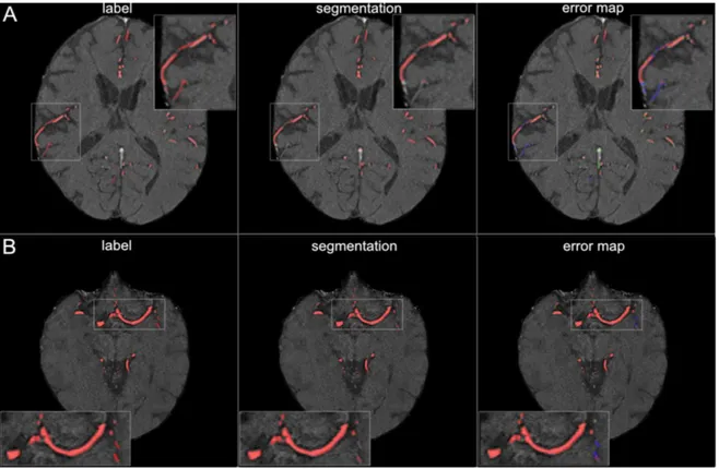
In [48], a specialized U-net architecture is implemented in 2D to perform a brain vessel segmentation for prevention and treatment in cerebrovascular disease in TOF-angiography. The results reported excellent performance in the large vessel and sufficient performance in small vessel segmentation as is possible to observe in Figure 2.1.2.

(29)

15

Figure 2.1.2: Segmentation results for small and large vessels. Figure A illustrates the segmentation results for small vessels, figure B for large vessel. The labels are shown in the first column of the figure and the segmentation results are shown in the second column. The third column shows the error map, where red voxels indicate true positives, green voxels false positives, and blue voxels false negatives. Adapted from [48].

In [49], a 30-layer 3D ResNet architecture is applied on 3D cerebral angiograms from a single contrast-enhanced C-arm cone-beam CT acquisition in patients with cerebrovascular abnormalities. The results, as it is possible to observe in Figure 2.1.3, reported excellent performance in vessel segmentation and reduction of image artifacts caused by misregistration of the mask. However, this study still has some limitations: the dataset used for model training, validation, and testing request manual editing before it can be used by the network and the 3D volumes used are region specific for a cerebrovascular zone of interest and so they do not contain the entire brain vasculature. Furthermore, it remains unknown if other architectures can be used and what would be the advantage or disadvantage among all these networks.

(30)

16

Figure 2.1.3: Comparison of anterior and lateral views of MIP images derived from 3D rotational angiography (A) and 3D Deep Learning Angiography (B) datasets of a patient evaluated for posterior cerebral circulation. It is possible to observe that the residual bone artifacts induced by patient motion are greatly reduced with the DL approach. Adapted from [49].

The improvement of the SEEG technique through an accurate vessel segmentation is the goal of this dissertation and nowadays, despite that several approaches have been proposed, no DL approach has been already tested in this specific framework.

In the “Claudio Munari” center for Epilepsy and Parkinson Surgery, the vessels are segmented by the neurosurgeons with a final manual threshold applied to the DSA, as already described in Section 1.2.

In [41] vessel are segmented from CT angiography images in two stages: first, the denoised CT Angiograms (CTA) is thresholded at the 97.5 percentile of the distribution of intensities; then, Frangi et al.’s filter is applied [20]. Even though this method captures the majority of the vessels, it tends to underestimate their width. Also in [50], vessels are segmented from phase-contrast magnetic resonance angiography (PC-MRA) images combining a multi-scale vessel enhancement filter [20], with a threshold process to reduce noise in the vessel images

(31)

17

and extract whole-brain vasculature. As before, this procedure suffers from an underestimation of the vessel’s width.

In [51], vessels are segmented from 3D phase contrast MRI (3DPC) and CT Angiograms (CTAs) using a multi-scale, multi-modal tensor voting algorithm: after optimal scale selection, images are converted into tokens (i.e., points) through analysis of the Hessian matrix; after voting, the resulting saliency maps are combined using the cosine between the vectors defining orientation, and the resulting probability map is then visualized in the planning system. Although this method is more accurate than a human observer using a single modality, the discontinuities appear in small branches vessel.

In [16], a Gaussian Mixture Model, modified to include neighborhood prior through Markov Random Fields (GMM-MRF), is used to robustly segment vessels and deal with the noisy nature of MIP images obtained from the first centimeter of the brain measured along the planned electrode direction. GMM-MRF privilege connected a set of pixels, compensating for the inaccurate vessel segmentation caused by noise or image inhomogeneities. Even though this method represents a completely automatic method able to identify vessel structures and compensate noisy pixels introduced by MIP, it suffers from vessel underestimation due to the connected nature of the brain vessel.

Despite these approaches being promising, first of all, the vessel segmentation technique applied in “Claudio Munari” center for Epilepsy and Parkinson Surgery is prone to error due to the fact that it is an operator-dependent technique. In fact, the final manual thresholding step needs an operator to be exploited, introducing noisy results or to lose thin vessels and losing morphological information. Secondly, all the other methods described in this framework used unsupervised approach or vessel enhancement techniques, which are more prone to the noise present in the data and also data specific. For these reasons and due to the complex morphology of cerebrovascular structures their translation into a gold standard clinical practice is hindered. On the other hand, it is clear that DL approaches demonstrate high effectiveness for vessel segmentation purposes, as described in Section 2.1, and so, they will be investigated and applied on the DSA to obtain the brain vasculature segmentation in this dissertation.

(32)

18

CHAPTER 3

MATERIAL AND METHODS

In this Chapter, the imaging acquisition technique and the pre-processing steps necessary to obtain the final training, validation and testing datasets from the patients' volumes collected from the “Claudio Munari” Center for Epilepsy and Parkinson Surgery, Niguarda Ca' Granda Hospital in Milan, will be presented in Section 3.1.

In Section 3.2, several FCNN architectures, that represents the DL reference to confront with, will be investigated.

In Section 3.3, the proposed method based on an ANN for brain vascular segmentation will be introduced in a 2D and 3D version in order to capture also the structural information of the brain vasculature.

Finally, in Section 3.4 the evaluation protocol used to evaluate the performance results of the brain vasculature segmentation will be investigated.

A graphical overview of the tested DL approaches is shown in Figure 3.1.2.

This work involved an anonymized dataset provided by “Claudio Munari” Center for Epilepsy and Parkinson Surgery, Niguarda Ca' Granda Hospital in Milan, acquired with O-arm System from 2017. All procedures were in accordance with the ethical standards of the institutional research committee, with the 1964 Helsinki Declaration and the Ethical approval was sought from the Niguarda Hospital Ethical Committee. Individual patient consent was obtained for the use of anonymized preoperative imaging. At the time of the acquisition, all patients did not present any vasculature pathologies and underwent the standard acquisition protocol for SEEG pre-operative planning.

(33)

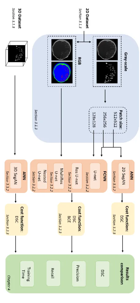
19 Figur e 3.1 .1 : W or kf low o f t he tes ted appro ache s for br ai n vas cu la r s egment at ion. The re su lts of th e ves sel s eg m ent at ion, ob tai ned w ith th e di ffer en t arc hi te ct u re s pro pose d in thi s C hapt er , w ill be compa red throu gh four pe rf o rmanc e m et ri cs : D ice Si m ila ri ty C oef fic ien t ( D SC ), Pre ci si on , Reca ll, Trai n ing tim e (h) .

(34)

20

In particular, the collected dataset is composed of 50 patients, and for each one, there are two different types of volumes:

• Bone Mask volumes (BM): preliminary CT that enhances only the bone;

• Contrast-Enhanced brain vessel volumes (CE): obtained during the infusion of an iodinated CM agent through the right/left internal carotid causing the enhancement of a hemisphere at a time, right or left respectively.

Each image volume has a voxel resolution of 0.415 x 0.415 mm in the axial plane and 0.833 mm in the z-direction, accounting for 192 slices, each of size 512 x 512 pixels. Considering a total initial dataset of 50 patients, only 38 of them were considered in this work. The excluded datasets were not in compliance with the investigated problem for different reasons, e.g., low image quality, modified acquisition protocol due to specific clinical scenarios. In this perspective, the dataset was divided into two folds: 33 patients were used for training and 5 for testing purposes only. Out of these 33 patients, we used 26 of them (~ 79% of the total number of patients) for training and 7 (~ 21% of the total number of patients) for validating the training phase, to avoid overfitting during the learning phase (Table 3.1.1).

Table 3.1.1: Number of patients used for the training, validation, and testing set.

Training Set Validation Set Test Set

26 Patients 7 Patients 5 Patients

These final datasets are obtained after some pre-processing steps (Figure 3.1.2) necessary to obtain the final binary segmentation mask of the DSA volumes, which represents the network ground-truth volumes keeping only the brain vascular tree. These pre-processing steps will be explained more in detail in Section 3.1.2.

(35)

21

Figure 3.1.2: Pre-processing workflow to obtain the binary segmentation of the Digital subtraction angiography (DSA) volumes. The DSA binary segmentation volumes represent the network ground truth. The 3D Bone Mask (BM) volumes, after registration to the 3D Contrast Enhanced (CE) volumes, will be subtracted from the CE volumes in order to obtain the DSA. The final 3D-Ground Truth will be obtained after a manual manipulation step followed by a binarization step on the 3D-DSA.

The image acquisition protocol to obtain a 3D angiography able to capture the brain circular system morphology is composed of the following steps:

a) positioning of the catheter into the femoral artery and then advanced into the internal carotid artery (ICA);

b) centering of the patient’s head in the gantry by means of 2D images;

c) connection of the catheter to the Mark V Provis Angiography Injection System; d) selection of the 3D acquisition protocol (Low Dose, Standard, High Definition, and

Enhanced). These protocols differ between them in terms of X-ray dose, the number of two-dimensional (2D) rotational projections generated and the quality of the 3D reconstruction that progressively increases from the Low Dose to Enhanced protocols (Figure 3.1.3) [15];

e) acquisition of the first 3D dataset, represented by the bone mask;

f) acquisition of the second 3D dataset during the injection of the contrast medium (CM, 300 mg/mL of iopamidole with a rate of 2 mL/s);

(36)

22

g) optional acquisition of the third 3D dataset during the injection of the CM in the contralateral Internal Carotid Artery (ICA) and/or vertebral artery (VA).

Figure 3.1.3: Standard or Enhanced acquisition protocol. The Enhanced protocol (left) produces images less affected by radial artifacts when compared with Standard protocol scans (right). Moreover, the Enhanced protocol provides better visualization of the soft tissue [6]. Reprinted from

[15].

The acquisitions are done with the mobile CBCT scanner. In particular, the O-arm system, a mobile intraoperative 2D/3D imaging system that is designed to meet the workflow demands of the surgical environment, is used. This system can be used in a variety of procedures (including spine, cranial, and orthopedics) and it offers options for workflow efficiencies, such as (Figure 3.1.4)[52]:

• it can be used to provide the initial dataset in procedures where pre-operative axial/coronal/sagittal slice data is necessary;

• it eliminates the need to send patients to be scanned in radiology; • it assures inter-room mobility for concurrent cases;

• it can be used intra-operative to obtain on-demand imaging;

• it can be used without the need to wear lead protective apparel during the navigated steps of the procedure thanks to the possibility to reduce the dose radiation;

• it assures flexibility to choose the appropriate dose (e.g., Low Dose, Standard Dose) to the patient, based upon individual clinical objectives

(37)

23

Figure 3.1.4: Workflow comparison between the standard surgical procedure and the O-arm system procedure. The O-arm system meets the workflow demands of the surgical environment decreasing the number of standard surgical procedures step from three to one. It can be used in a variety of procedures including the spine, cranial, and orthopedics exams. Reprinted from [52].

More in detail, the O-arm is composed of an X-ray tube and a flat panel detector isocentrically rotating inside a circular gantry (Figure 3.1.5). While rotating 360 degrees around the subject, it acquires up to 390 X-ray projection images over 12 seconds that will serve as a basis for the 3D CT reconstruction. This device uses a cone-shaped X-ray beam that allows for the obtaining of a scan of the entire head with a single rotation of the gantry (exposition to the entire Field of View (FOV)), instead of conventional CT scanners which uses a fan X-ray beam. In this way, thanks to cone-beam geometry, is possible to achieve scan time generally lower than 1 minute [53].

Figure 3.1.5: CT cone-beam acquisition geometries. This method allows obtaining a scan of the entire head with a single rotation of the gantry. Reprinted from [53].

(38)

24

The training inputs of the networks, as introduced in Section 3.1, are the CE-CBCT volumes and the binary segmentation mask of the DSA volumes, which represent the ground truth volumes. In particular, the networks have to reproduce as output these ground truth volumes in the best possible way.

In order to obtain the final ground truth volumes, we apply four main steps on the two volumes collected from the “Claudio Munari” center for Epilepsy and Parkinson Surgery:

1. rigid-body registration: it was applied because, during the acquisition of the BM and CE-CBCT volumes, possible patient interscan motion might occur. For this purpose, FLIRT (FSL) software, a fully automated robust and accurate tool for linear (affine) intra- and inter-modal brain image registration, was used. In detail, the BM volumes are transformed in BMCE to physically match the CE-CBCT volumes;

2. images subtraction: the CE-CBCT volumes were subtracted to the BMCE volumes (BM obtained after the registration) in order to obtain the DSA volumes, preserving only the brain vascular tree;

3. manual manipulation: an eye threshold was applied to remove the background noise present in the DSA volumes, as is possible to observe in Figure 3.1.6. For this purpose, the ITK-snap [54] software, was used. It is especially used to segment structures in 3D (i.e., medical images) and compare them with the result of other open-source image analysis tools.

4. image binarization: it was applied to the DSA pre-segmented volumes, through ITK-snap software, to achieve better segmentation results with the implemented networks. In detail, new volumes in which each voxel equal to 1 univocally represents the presence of vessel, and each voxel equal to 0 represents the absence of them was created. For this purpose, the Matlab R2018b software was used. In particular, the function imbinarize with the “adaptative” method and the function bwconncomp were applied.

(39)

25

Figure 3.1.6: Result of a DSA volume manually thresholded. Digital subtraction angiography (DSA) volume on the left part of the figure, DSA volume manually thresholded (‘Speed Image’) with ITK-snap on the right part of the figure.

After these pre-processing steps, the final DSA ground truth (GT) volumes were qualitatively checked and missing vessels were manually segmented. This final step is done in order to improve the quality of the GT provided to the network but is not performed in the imaging pipeline proposed at the “Claudio Munari” center for Epilepsy and Parkinson Surgery.

Considering the CE-CBCT volumes and the relative GT volumes created, two different types of training, validation, and testing datasets were generated from the 38 patients dataset: a 2D and a 3D version of the training dataset. In particular, the 2D datasets were generated saving each patient volume slice as a .png format image: the CE-CBCT images were generated with pixel range values between {0-255}, the binary GTs were generated with pixel values of 0 or 255.

(40)

26

Different versions of the 2D datasets were created (Figure 3.1.7):

• 1-channel dataset: composed of CE-CBCT images and the respective grey scale-GT images characterized by a size of 512x512 pixels;

• 1-channel 256x256 patches dataset: composed of CE-CBCT patches images and the respective grey scale-GT patches images characterized by a size of 256x256 pixels. All the patches images were generated with an overlap size of half of their final pixel size. Furthermore, the all-black CE-CBCT patches images and the corresponding GT patches images were eliminated from this dataset;

• 1-channel 128x128 patches dataset: composed of CE-CBCT patches images and the respective grey scale-GT patches images characterized by a size of 128x128 pixels. All the patches' images were generated with an overlap size of half of the size of their final pixels. The all-black CE-CBCT patches images, and their corresponding GT patches images were removed from this dataset. Furthermore, the final dimension of the dataset has been reduced, to decrease the too high number of images generated which would have resulted in too longer computation time (more than 5 days). In order to do this, we randomly eliminated the CE-CBCT patches images, and the corresponding GT patches images;

• 3-channels dataset: composed of CE-CBCT images characterized by a size of 512x512 pixels and the respective RGB scale-GT images characterized by a size of 512x512x3 pixels. The third size dimension represents the number of present channels. In detail, the first channel represents the vessel, the second one represents the bone mask and the third one represents the soft tissue mask.

To obtain 3-channels in the ground-truth images a data manipulation followed by a data binarization, already introduced in Section 5.1.2, of the registered BM volumes, was necessary. After that, we obtained the segmentation mask of the soft tissue multiplying the complement of both the segmented DSA volumes and the segmented BM volumes to the CE-CBCT volumes. Finally, we binarized the soft tissue mask to be consistent with the other channels, and then we concatenated the three-channel created in the third dimension.

(41)

27

Figure 3.1.7: 2D datasets. For each 2D dataset, the Contrast enhanced cone-beam computed tomography (CE-CBCT) images and the corresponding Ground Truth (GT) are represented. In the final datasets, the all-black CE-CBCT patches images and the corresponding GT patches images were eliminated.

The 3D dataset was generated following four steps procedure:

• resize of each patient volume of 512x512x192 voxels in 348x448x192 voxels, to reduce the background region of the volume;

• volumes patches generation of size 176x224x64 voxels for each patient, which represents the maximum value that fits the GPU memory. All the patch volumes were generated with an overlap size of half of their final voxel size.

• removal of black patch volumes in each patient;

• save each patient volumes in a .npy format array: the CE-CBCT volumes were generated with voxel range values between {0-255}; the GT volumes were generated with voxel values of 0 or 255.

In detail, as reported inTable 3.1.2, for the training dataset we have: 4,992 images for the 2D 1-channel and 3-channel dataset, 40,528 patches images for the 2D 1-channel 256x256 patches dataset, 60,000 patches images for the 2D 1-channel 128x128 patches dataset and 1,010 volumes for the 3D dataset.

(42)

28

For the validation dataset we have: 1,344 images for the 2D 1-channel and 3-channel datasets, 8,096 patches images for the 2D 1-channel 256x256 patches dataset, 25,856 patches images for the 2D 1-channel 128x128 patches dataset and 302 volumes for the 3D dataset. For the testing dataset, the first 46 slices and the last 20 ones for each patient were deleted; in fact, these slices did not contain vessel information (all black slices) or presented misregistration errors such as the mandible, the nose, and the eyeballs (Figure 1.2.2). Hence, for the testing dataset we have: 640 images for the 2D 1-channel and 3-channel datasets, 3,582 patches images for the 2D 1-channel 256x256 patches dataset, 20,145 patches images for the 2D 1-channel 128x128 patches dataset and 225 volumes for the 3D dataset.

Moreover, during the testing phase, only the CE-CBCT images/volumes were used as input of the networks, while the GT images/volumes were used to compare the results obtained from the networks.

Table 3.1.2: Summary of the training, validation and testing datasets generated. For each dataset, the dimensionality, the number of channels, the size and the number of elements present are shown.

In this Section after a brief introduction to the main concept of Fully Convolutional Neural Network (FCNN, Section 3.2.1), the proposed reference architectures will be presented in

Dimensionality Channels CE-CBCT

(size) GT (size) Training dataset n° elements Validation dataset n° elements Testing dataset n° elements 2D 1 channel 512x512 512x512 4 992 1 344 640 1 channel 256x256 256x256 40 528 8 096 3,582 1 channel 128x128 128x128 60 000 25 856 20,145 3 channels 512x512 512x512x3 4 992 1 344 640 3D 1 channel 176x224x64 176x224x64 1 010 302 225