Disclosing Brain Functional Connectivity from Electrophysiological
Signals with Phase Slope Based Metrics
A. Basti1*, V. Pizzella1,2, G. Nolte3, F. Chella1,2 , L. Marzetti1,2
1 Department of Neuroscience, Imaging and Clinical Sciences, G. d'Annunzio University of Chieti-Pescara, 66100 Chieti, Italy
e-mail: [email protected]
2 Institute for Advanced Biomedical Technologies, G. d'Annunzio University of Chieti-Pescara, 66100 Chieti, Italy
3 Department of Neurophysiology and Pathophysiology, University Medical Center Hamburg-Eppendorf, D-20246 Hamburg, Germany
*corresponding author
Abstract
The characterization of the coupling direction between brain regions is fundamental for disclosing brain functioning. To this end, several computational methods have been developed that exploit either the temporal or the spectral characteristics of electrophysiological signals measured by e.g. EEG and MEG. Among these methods, the Phase Slope Index (PSI) estimates the directionality of frequency-specific neural interactions by relying on the sine of the phase slopes of the complex coherencies between time series, which is just an approximation for small angles of the actual phase slopes. The purpose of our study is to: 1) build a directionality estimator, namely id, which directly takes into account the non-approximated phase slopes; 2) assess the performance in estimating the coupling direction of PSI and id in exhaustive simulations. Our findings show that while id obtains better performance than PSI for the no noise case, a Signal-to-Noise Ratio equal or lower than one completely reverses the results in favour of PSI.
Keywords: Brain functional connectivity, phase slope index, coupling direction.
1. Introduction
The development of signal processing techniques plays an increasingly fundamental role in the fields of neuroscience and neural engineering (Berger et al. 2010, Hyvärinen et al. 2004, Marzetti et al. 2008, Power et al. 2014). Indeed, the application of advanced processing methods to functional neural imaging data can provide fundamental insights on brain functioning in health and disease. Specifically, recent holistic approaches to neuroimaging focus on the functional relations between different brain areas, commonly referred to as brain functional connectivity, to understand how the complex human behaviour is realized. In this framework, a key issue in the development of those computational methods is the determination of the directionality of brain areas interaction (Baccalá and Sameshima 2001, Chen et al. 2006, Friston et al. 2003, Marinazzo et al. 2008, Nolte et al. 2008, Rosenblum and Pikovsky 2001). Being able to disclose the directionality of neural couplings is fundamental for the
understanding of large scale information processing in the brain (Babiloni et al. 2005, Hillebrand et al. 2016) thus permitting to disentangle feedback and feedforward functional pathways (Varela et al. 2001). Understanding the directionality of connections would thus allow to reveal the dynamical functional relationships between brain areas established during cognitive processing. To this end, a noninvasive functional imaging technique allowing for a direct measurement of the brain electrophysiological activity and with a millisecond time resolution, such as MagnetoEncephaloGraphy (MEG) or ElectroEncephaloGraphy (EEG), is needed (Baillet 2017, Hämäläinen et al. 1993) as well as the development of specific analysis methods.
A feature of neural interactions which enables a method to identify driver and receiver roles of specific brain regions in the coupling, is the noninstantaneous temporal propagation among functional connected brain areas. Namely, the synchronization among brain regions occurs with time lags (Fries 2015) which range from a few milliseconds up to a hundred of milliseconds (Baldauf and Desimone 2014, Bastos et al. 2015, Tass 2007). As we will discuss in more detail in the next paragraph, the presence of such nonzero time lags leads to a nonzero frequency derivative of the phase difference between two-time series, i.e. phase slopes, whose values directly depend on those delays, and whose sign reveals the directionality of the underlying interaction. This is the idea behind the formulation of the Phase Slope Index (PSI) (Nolte et al. 2008), one of the most robust and reliable methods currently available to disclose the directionality of frequency-specific neural interactions. Indeed, PSI is basically a weighted sum of the approximate phase slopes. PSI was tested in simulations (Haufe et al. 2013, Nolte et al. 2010) and successfully used to establish directionalities from neurobiological time series, e.g. resting state subdural ElectroCorticoGraphy (ECoG) (Casimo et al. 2016), subthalamic Local Field Potential (LFP) (Hohlefeld et al. 2013), task MEG (Kadis et al. 2016) as well as resting state EEG (Nolte et al. 2008).
In this paper, we build a new directionality estimator, based on the PSI concept, in which the small angles approximation used in PSI is avoided and we test if the estimation of the direction of coupling can be improved in this way.
1.1 Phase slope and directionality
We aim here at clarifying how the sign of the frequency derivative of the phase difference between two-time series informs about temporal precedence, i.e. directionality. A common way to assess the phase difference between two-time series is to estimate the phase of their cross-spectrum. If we assume a temporal precedence between the twotime series, say one is the driver and the other is the receiver, and considering a time lag between the former and the latter, then the phase differences between them increases with the increase of frequency, i.e. in such a way that the phase slopes of the cross-spectrum between the driver and the receiver is positive.
In order to better understand this concept and thus define the PSI, let us consider two signals x and y such that
( ) ( ),
y t ax t (1)
where (τ,a)∈ x . From (1), it follows that between x and y there is a causal relationship; in particular, if is positive, x is the driver and y is the receiver; while negative values of imply the opposite. The absolute value of is the time delay of the coupling.
In the Fourier domain, the relationship between the two signals expressed in (1) becomes y f( )aei2 f x f( ) and the cross-spectrum, i.e. *
( ) ( ) x f y f
where denotes the expectation value and * the complex conjugation, turns out to be equal to
*
( ) ( ) ( )
i f
ae x f x f where ( ) : 2 f f is the phase difference between x and y at the frequency f.
Given that ( ) f is a linear function of the frequency, we have that the phase slope, given by d ( ) : d ( f f d ) d ( )f f , where df is an incremental step in frequency, is constant and frequency-independent, in fact
d ( ) 2 ( f f d )f 2 f 2 d . f (2) This means that the sign of d ( ) f informs about the role played by x and y in the coupling. In fact, since df is positive, we have that the sign of d ( ) f is totally determined by the sign of , and vice versa. Thus, a positive phase slope implies a positive meaning that x is the driver, while a negative phase slope implies negative , i.e., x is the receiver. See Fig. 1 for a schematic representation of the phase slope.
Fig. 1. Slope of the phase differences between a signal and its delayed version.
The PSI (Nolte et al. 2008) is a measure of directionality based on the above concept. Specifically, PSI exploits the sign of the sine of the phase slopes of the cross-spectrum between two time-series given that, for small angles, this is equal to the sign of the phase slopes. Indeed, an estimate of the phase slope d ( ) f can be obtained by relying on the imaginary part of the product of coherencies between x and y, i.e. cross-spectrum divided by the square root of the product between the power-spectra, at frequencies f+df and f as expressed below in (3). By calculating this product, we have that
* 2 ( ( d ) ( )) , , Im(Cx y(f d )f Cx y( )) Im(f ei f f f ) 2 d ( ) Im(ei f ) sin(d ( )) d ( )f f (3)
where sin(d ( )) d ( ) f f is the small-angle approximation which holds for small df . In Eq. (3) we have used that the complex coherency Cx y, ( )f , obtained by dividing the cross-spectrum by the square root of the product between the power-cross-spectrum of x and y, can be written as
* 2 2 ( ) , ( ) * ( ) ( )* . ( ) ( ) ( ) ( ) i f i f i f x y ae x f x f C f e e a x f x f x f x f (4)
Nevertheless, in general, an interaction between a driver and a receiver leads to more complex expressions for the relationship between the two signals than the ones considered in (1). This means that, e.g. the magnitude of Cx y, (f d )f C*x y, ( )f could be different from 1 and
1
d ( ) f different from d ( ) f2 if the two frequencies f1 and f2 are such that f1 f2. A good strategy to take into account the above considerations when using the phase slopes for estimating the directionality is to perform a sum over a set of frequency of interest in a range F, i.e.,
*
* , , , , : Im x y( d ) x y( ) | x y( d ) x y( ) | sin(d ( )). f F f F C f f C f C f f C f f
(5)This allows to obtain a weighted sum of the approximate phase slopes, which considers different frequencies according to the statistical relevance and which vanishes for mixture of independent noise sources (Nolte et al. 2004). The PSI is defined as the standardized version of (5), that is PSI : / std( ) where the estimate of std( ) can be obtained by e.g. the Jackknife method.
We recall that the sine of the phase slopes, used in (5) to define the PSI, represents only an approximation of the actual phases of the products of coherencies. The aim of this paper is twofold. First, we will build a directionality estimator, namely id, which takes directly into
account the non-approximated phase slopes. Second, we will assess the performance in estimating the coupling direction of PSI and ofid in exhaustive simulations.
The paper is organized as follows. In the Methods sections, we will introduce the definition of the non-approximated estimator of phase slopes (Section 2.1), and describe the interaction model set up to mimic directional brain areas coupling, as measured from electrophysiological sensors, with different time delay values and different level of the SNR associated with the correlated noise, which is known to have a weight on sensor level larger than the weight of the uncorrelated noise (Section 2.2). In the next two paragraphs of the same section, the practical setting for the directional coupling estimation and the criteria for performance evaluation are presented, respectively. The Results for the two approaches are then shown and discussed and, finally, future perspective for phase slope based approaches are drawn.
2. Methods
2.1 Definition of id as the weighted sum of the actual phase slopes
We will show that it is possible to calculate the phase slopes
d ( ) f
f F assuming that each of them lies in the interval ( , ). This strategy allows to completely avoid the small-angle approximation used in PSI and to define a method for directionality estimation which is the based on a weighted sum of the actual (i.e., non-approximated) phase slopes.In fact, depending on the signs of the real and the imaginary parts of the products of coherencies, we have that
* , , * , , * , , * , , * , , * , , if Re( ( d ) ( )) 0 if Re( ( d ) ( )) 0 Im( ( d ) ( )) arcsin | ( d ) ( ) | Im( ( d ) ( )) arcsin | ( d ) ( ) | d (f)= x y x y x y x y x y x y x y x y x y x y x y x y C f f C f C f f C f C f f C f C f f C f C f f C f C f f C f
* , , * , , * , , * , , and Im( ( d ) ( )) 0 if Re( ( d ) ( )) 0 Im( ( d ) ( )) arcsin | ( d ) ( ) | x y x y x y x y x y x y x y x y C f f C f C f f C f C f f C f C f f C f
* , , and Im(Cx y(fd )f Cx y( )) 0f (6)where Re indicates the real part of a complex number and Im its imaginary part as above. The modified PSI which directly considers the d ( ) f values, and which corresponds to the weighted sum of the actual phase slopes, can therefore be defined as
* , , : | ( d ) ( ) | d ( ). id x y x y f F C f f C f f
(7) id can be thought as a modified PSI in which, in place of the sine function, there is the identity function of the phase slopes, i.e. the function id: ( , ) ( , ) such that
(d (f)) d (f)
id . This is the reason why we used the subscript id in terming this estimator
id
. As for PSI, to assess a statistical significance in the observed results, it is better to consider a standardized version of , id id :id / std(id). A complete description of a possible approach to estimate the standard deviation is provided in Section 2.3.
The precise calculation of the phase of a given signal is not possible in noisy environments and thus, for real data, the estimate of the phase will be perturbed with respect to the real unknown value. This would mean that also the calculation of sin(d ( )) f , that appears in the definition of the PSI, will be perturbed by the presence of noise. Nevertheless, it is important to note that the use of trigonometric inversion such as the one used in (6) does not introduce further errors, given that this approach is merely based on the application of trigonometric functions; hence the same kind of perturbation which afflicts the original PSI afflicts the calculation of the phase slopes in (6) and thus the calculation of in (7). When using the term id
"actual" phase slope referred to the definition of we do not mean that the method is able to id exactly reconstruct the real unknown phase, rather we imply that an exact mathematical expression for the phase is used in its definition in place of the approximated expression used by the PSI.
2.2 Synthetic interaction model
The sets of data here simulated to test the performances of the two methods consist in pairs of time series which mimic the evolution of sensor signal pairs as a weighted superposition of the interaction of two directionally connected sources with biological noise terms. The interaction model that we built in this study, schematically depicted in panel a) of Fig. 2, aims at
resembling the situation in which two sources are coupled in the brain with some temporal precedence between them, and the available information to estimate this coupling are data as measured from scalp electrophysiological sensors outside the brain. We further assume that, consistently with a realistic case, the sensors measure not only the interacting source activity but also the activity of uncorrelated brain noise.
Each pair of time courses z( , )x yT is thus defined as the following bivariate time series of length L, F F ( ) ( ) ( ) (1 ) s t n t . z t S N (8)
In (8), the components of ( ) ( ( ), ( ))s t d t r t Trepresent the signals generated respectively by the driver ( )d t and the receiver ( )r t at the discrete time t, and reflect the interaction between brain sources the direction of which we are interested to detect. The term n t( ) simulates biological noise as the instantaneous mixing of the evolution of three neural sources at t, independent between them and with respect to the driver and receiver sources. S andF
F
N are the Frobenius matrix norms of S[ (1),..., ( )]s s L , and N [ (1),..., ( )]n n L . The coefficient[0,1] indicates the noise strength defining the Signal-to-Noise Ratio (SNR), e.g., a value forequal to 0.5 means a balanced contribution between signal and noise for the sensor signal pair zand, consequently, a SNR equal to 1. An example of sensors time series is shown in the panel b of Fig. 2.
Fig. 2. Graphical representation of the interaction model and example of sensors time series The evolution of the signal term is modeled according to
1 ( ) ( ) ( ) Q k k k d t a d t h t
(9)( ) ( ) ( )
r t bd t t (10)
for the receiver; while the noise evolution is modeled as
1, 1 1 1 2, 2 2 1 3, 3 3 1 ( ) ( ) ( ) ( ) ( ) . ( ) ( ) Q k k k Q k k k Q k k k c n t h t n t B c n t h t c n t h t
(11)In (9), (10) and (11), Q is a positive integer and a , b, c , ( ), ( ), ( )k i k, t t i t , with k=1,…,Q and i=1,2,3, as well as the components of the mixing matrix B∈ 2x3, are realizations of independent normal random variables.
Each time courses generated in this study is sampled at 254 Hz, it has a length of L=15240 data points corresponding to a 1 min of continuous measurement each, and it is obtained by setting in (9) and (11), Q=5 (Haufe et al. 2013; Haufe and Ewald 2016) and hk 3.9kms. In this study, we generated a total of 36000 pairs of time series. Specifically, we generated the synthetic data as 30 sets of 100 pairs of time courses for each of the twelve values considered for the time delays. Given that the physiological time delays between the driver and the receiver sources range from a few milliseconds up to a hundred of milliseconds (Baldauf and Desimone 2014, Bastos et al. 2015, Tass 2007), we chose to vary the time lags in the model (denoted by ) in (10) from 7.8 ms to 93.6 ms with an incremental step of 7.8 ms. All the time series d, r and
i
n with i=1,..,3 are bandpass filtered in the gamma band (25-40 Hz) by using a IIR Butterworth filter with zero phase delay implemented in FieldTrip toolbox (Oostenveld et al. 2011).
Finally, the value is set to 0.5, i.e. a SNR equal to 1, for all the simulations with noise. This situation is aimed at resembling a poor SNR condition which reflects the coupling between the high frequency weak signals observed when the brain is in the so called resting state condition, i.e., wakeful relax state in which no specific stimulus is presented to the subject and no task is required to be performed.
2.3 Parameter settings for the estimation of PSI and id
To calculate the spectral coherencies in (5) and (7), we first divided each time series into 30 epochs of the same length, containing 2 seconds of continuous data, and we further divided each epoch into 3 segments of 1 second duration, with 50% overlap, which corresponds to a frequency resolution df equal to 1 Hz. We multiplied the data of each segment with a Hanning window and finally estimated the power/cross-spectra as an average of the products of the Fourier transforms over all segments (Nolte et al. 2008).
To assess the statistical significance of the observed PSI and id results, we firstly normalized
the measures by an estimation of their standard deviations calculated by using the Jackknife method (Nolte et al. 2008, Nolte et al. 2010). Specifically, in this work, the standard deviation of e.g. is defined over a set of its estimates each, termed here id with j=1,...,30, obtainedidj
from the data in which the j-th epoch has been removed. The standard deviation of is thus id finally estimated as 30 where is the standard deviation of the set
1 ,..., 30
id id
.
By interpreting this normalization strategy as a pseudo-Z score, it is possible to fix a level of significance and thus to read the observed p-values according to a Gaussian distribution. Here, we chose 1.96 as the threshold value corresponding to a level of significance of 0.05 (two-tailed). This means that, if the absolute value of PSI or of id exceeded 1.96, the direction of coupling detected by the sign of the method was considered as significant.
2.4 Performance evaluation
The approach we pursued here to evaluate the performance of the connectivity methods is that of considering its Mean Squared Error (MSE) in estimating the directionality.
Specifically, for each of the 30 sets of 100 pairs of time series and for each of the twelve time delays considered in this study, we calculated the MSE in estimating the parameters
i where i
1,1 describe if the direction of the i-th simulated interaction is source1-to-source2, e.g. i 1, or source2-to-source1, e.g. i 1. Specifically,2 2 (sgn(PSI( ))- ) MSE(PSI) MSE( ) (sgn( ( ))- ) i i id id i i i i
(12)where e.g. sgn(PSI( ))i is equal to 1 , respectively, if a statistical significant source1-to-source2 or source1-to-source2-to-source1 direction for the i-th coupling is detected by PSI, while, it is equal to 0 if the detected directionality is considered as not statistically significant.
Hence, a value for the ratio between the MSEs, termed MSE ratio in the following, larger than 1 implies, for that time lag, a better performance of id over PSI, while a value smaller than 1 implies a better performance of PSI over id. For each time delay value considered, a two-sided sign test, which tests the hypothesis that the ratio between MSEs has median equal to 1 against the alternative that its distribution does not have median equal to 1, is used.
The codes for PSI and id calculation were implemented in Matlab (R2012b, The
Mathworks, Inc., Natick Massachusetts, United States). The computational cost for the calculation did not significantly differ between the two estimators. Indeed, for each pair of time series, PSI required roughly 60 ms and id roughly 61 ms on a desktop PC (Intel® i7-6700
CPU @ 3.40 GHz; RAM 16 GB).
3. Results and discussion
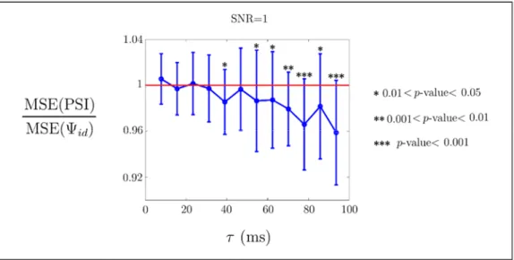
Figure 3 shows the average (denoted by the dots) and standard deviation (denoted by the bars) of the MSE ratio as a function of the time lag value between the driver and the receiver, obtained from data simulating a realistic noisy situation (SNR=1). Furthermore, significant p-values for the two-sided sign tests are shown.
From Fig. 3, it is evident that the difference in the performance between PSI and id
depends on the value. Indeed, while for smaller than 40ms there is no statistically significant difference between them, a significantly better behaviour of PSI is observed for larger values of .
Fig. 3. Ratio between the Mean Squared Error (MSE) of PSI and for SNR=1 id
To answer the question whether PSI has obtained better performance, for large , because of its higher ability in facing the effects of the biological noise, we generated a total of 36000 pairs of time series in a situation with SNR , i.e. a value equal to 0 in the model (8). This situation can resemble, as opposite to the previous one, the situation of very high SNR as that obtained in the study of evoked brain activity in which multiple repetitions of the same stimulus are presented to the subject or multiple instances of the same task are performed by the subject, e.g., high frequency activity related to visual stimulation. If the same results obtained for SNR=1 were observed for SNR , this would suggest that the PSI would have better performance than regardless of the noise level. id
Conversely, Fig. 4 shows a different result with respect to the one shown in Fig. 3. Indeed, the ratio between the MSEs for SNR is significantly larger than 1 for the most of the values, meaning that has obtained better performance than PSI. id
Furthermore, it is worth to notice that the MSE of the both methods decreases as the increase of the time delay value, e.g., PSI has obtained a percentage which goes from about 80% to about 40% with a SNR=1 and from about 40% to about 15% with a SNR=.Those results are in accordance with the fact that the larger the time delay, the larger the phase slope (equation 2), provided the time delay value does not lead to a change of sign due to the exceeding of the value.
Fig. 4. Ratio between the Mean Squared Error (MSE) of PSI and for SNR= id When, for a representative time delay larger than 40 ms, the noise contribution is parametrically increased, i.e., is increased by steps of 0.1, the ratio of MSEs decreases towards the reversed situation obtained for SNR=1. This is shown in Fig. 5 for a representative case, i.e., 70ms.
Fig. 5. Ratio between the Mean Squared Error (MSE) of PSI and for a time delay value of id
70ms
Taken together our findings show that obtains better performance than PSI for high id SNR, while the presence of biological noise, which in this study is simulated as the
contribution to the sensors of the mixing of three independent neural sources, negatively affects the performance of id. Indeed, in this case PSI results to be a better estimator of the
directionality of interactions for delays larger than 40 ms, while no statistical difference between the two estimators is found for smaller delays.
A reasonable explanation of why a weighted sum of the approximated phase slopes, i.e. PSI, behaves better than the weighted sum of the actual phase slopes, i.e. id, might be found in the shape of the phase slopes functions in id and in PSI. Indeed, as we previously noted,
id
can be thought as a modified PSI in which, in place of the sine function, there is the identity function of the phase slopes. The direct proportionality between the angles and the weights that the identity function in id gives to those phase slopes can be the reason why PSI
has obtained higher performance than id in the presence of noise term. In fact, the function in the latter measure assigns the largest weights to the phase slopes around leading to unstable estimates of the directionality given the possible phase jumps from 0 to in the presence of mixture of independent noise sources. Conversely, PSI reduces these instable estimates by weighting with small values large phase slopes.
Finally, even though we have used matrices which randomly mix the independent noise sources, we do think that the obtained results do not depend on specific definitions of that matrix and, thus, that results similar to those obtained in this study would have been obtained e.g. by a priori fixing an electrophysiological technique with a realistic head/forward model (i.e., by fixing a specific mixing matrix).
4. Conclusions
The Phase Slope Index (PSI) (Nolte et al. 2008) is an estimator of the direction of brain areas coupling from electrophysiological time series. Specifically, PSI is the weighted sum of the phase slopes, i.e. of the discrete derivatives with respect to frequency of the phase difference between the two time-series, approximated by using the sine function. In this work, we have introduced and tested, in exhaustive simulations, a modified version of PSI which corresponds to the weighted sum of the actual phase slopes. We termed this measure as id.
Our findings proved that id obtains better performance than PSI in the absence of noise,
while the presence of biological noise completely changes the results. Indeed, a balanced contribution between signal and noise makes PSI a better estimator of the direction of coupling. In conclusion, unless the presence of the biological noise, such as the effects of the volume conduction or the source leakage effects (Palva and Palva 2012) can be excluded, e.g. by considering situations in which the SNR is known to be high or by using a computational approach to reduce the correlated noise contribution (O’neill et al. 2015), the use of PSI on real study should be preferred.
The sine function used in the formulation of PSI, as well as the identity function used in definition ofid, can be seen as two out of all the possible weight functions of the phase slopes which can be defined. In future studies, it is important provide answer to the question whether it is possible to define a weight function of the phase slopes to obtain the best performance in disclosing directionality in comparison with the two tested here.
A worth further direction to take is that of focusing on the development of a multivariate extension of the phase slope based metrics, which could take into account the multidimensionality in the data in a way similar to that of the generalization of the imaginary
part of coherency method termed as multivariate interaction measure (Ewald et al. 2012). Indeed, both PSI and id are bivariate estimators of directionality and, thus, they rely on the
assumption that the signals are scalar quantities. Nevertheless, while this assumption is valid for e.g. MEG/EEG sensor signals, given that those signals are one-dimensional, it is a clear oversimplification for brain level data estimated through MEG/EEG inverse process, which reflect the evolution of current dipoles along three directions in the space.
References
Babiloni F, Cincotti F, Babiloni C, Carducci F, Mattia D, Astolfi L, Basilisco A, Rossini PM, Ding L, Ni Y, Cheng J, Christine K, Sweeney J, and He B (2005). Estimation of the cortical functional connectivity with the multimodal integration of high-resolution EEG and fMRI data by directed transfer function, Neuroimage, 24, 1, 118-131.
Baccalá LA and Sameshima K (2001). Partial directed coherence: a new concept in neural structure determination, Biol Cybern, 84, 463-474.
Baillet S (2017). Magnetoencephalography for brain electrophysiology and imaging, Nat. Neurosci., 20, 3, 327-339.
Baldauf D and Desimone R (2014). Neural mechanisms of object-based attention. Science, 344, 6182, 424-427.
Bastos AM, Vezoli J, Bosman CA, Schoffelen JM, Oostenveld R, Dowdall JR, De Weerd P, Kennedy H and Fries P (2015). Visual areas exert feedforward and feedback influences through distinct frequency channels. Neuron, 85, 2, 390-401.
Berger TW, Chen ZS, Cichocki A, Oweiss KG, Quian Quiroga R, and Thakor NV (2010). Signal processing for neural spike trains. Comput. Intell. Neurosci.
Casimo K, Darvas F, Wander J, Ko A, Grabowski TJ, Novotny E, Poliakov A, Ojemann JG and Weaver KE (2016). Regional Patterns of Cortical Phase Synchrony in the Resting State, Brain Connec. 6, 6, 470-48.
Chen Y, Bressler SL and Ding M (2006). Frequency decomposition of conditional Granger causality and application to multivariate neural field potential data, J Neurosci Methods, 150, 2, 228-237.
Ewald A, Marzetti L, Zappasodi F, Meinecke FC and Nolte G (2012). Estimating true brain connectivity from EEG/MEG data invariant to linear and static transformations in sensor space. Neuroimage, 60, 1, 476-488.
Fries P (2015). Rhythms for cognition: communication through coherence, Neuron, 88, 1, 220-235.
Friston KJ, Harrison L and Penny W (2003). Dynamic causal modelling, Neuroimage, 19, 4, 1273-1302.
Hämäläinen M, Hari R, Ilmoniemi RJ, Knuutila J and Lounasmaa OV (1993). Magnetoencephalography—theory, instrumentation, and applications to noninvasive studies of the working human brain. Rev. Mod. Phys., 65, 2, 413.
Haufe S, Nikulin VV, Müller KR, and Nolte G (2013). A critical assessment of connectivity measures for EEG data: a simulation study, Neuroimage, 64, 120-133, 2013.
Haufe S and Ewald A (2016). A simulation framework for benchmarking EEG-based brain connectivity estimation methodologies, Brain. Topogr.,1, 18.
Hillebrand A, Tewarie P, van Dellen E, Yu M, Carbo EWS, Douw L, Gouw AA, van Straaten, ECW and Stam CJ (2016). Direction of information flow in large-scale resting-state networks is frequency-dependent, Proc. Natl. Acad. Sci. USA, 113, 14, 3867-3872.
Hohlefeld FU, Huchzermeyer C, Huebl J, Schneider GH, Nolte G, Brücke C, Schönecker T, Kühn AA, Curio G and Nikulin VV (2013). Functional and effective connectivity in
subthalamic local field potential recordings of patients with Parkinson’s disease, Neuroscience, 250, 320-332.
Hyvärinen A, Karhunen J and Oja E (2004). Independent component analysis (Vol. 46). John Wiley & Sons.
Kadis DS, Dimitrijevic A, Toro-Serey CA, Smith ML and Holland SK (2016). Characterizing Information Flux within the Distributed Pediatric Expressive Language Network: A Core Region Mapped Through fMRI-Constrained MEG Effective Connectivity Analyses, Brain Connec., 6, 1, 76-83.
Marinazzo D, Pellicoro M and Stramaglia S (2008). Kernel method for nonlinear granger causality, Phys. Rev. Lett., 100, 14, 144103.
Marzetti L, Del Gratta C and Nolte G (2008). Understanding brain connectivity from EEG data by identifying systems composed of interacting sources. Neuroimage, 42, 1, 87-98.
Nolte G, Bai O, Wheaton L, Mari Z, Vorbach S and Hallett M (2004). Identifying true brain interaction from EEG data using the imaginary part of coherency, Clin. Neurophysiol., 115, 10, 2292-2307.
Nolte G, Ziehe A, Nikulin VV, Schlögl A, Krämer N, Brismar T and Müller KR (2008). Robustly estimating the flow direction of information in complex physical systems, Phys. Rev. Lett., 100, 23, 234101.
Nolte G, Ziehe A, Krämer N, Popescu F and Müller KR (2010). Comparison of Granger Causality and Phase Slope Index, NIPS Causality: Objectives and Assessment, 267-276. O’Neill GC, Barratt EL, Hunt BA, Tewarie PK and Brookes MJ (2015). Measuring
electrophysiological connectivity by power envelope correlation: a technical review on MEG methods. Phys. med. biol., 60, 21, R271.
Oostenveld R, Fries P, Maris E and Schoffelen JM (2011). FieldTrip: open source software for advanced analysis of MEG, EEG, and invasive electrophysiological data, Comput. Intell. Neurosci.
Palva S, and Palva J M (2012). Discovering oscillatory interaction networks with M/EEG: challenges and breakthroughs. Trends. Cogn. Sci., 16, 4, 219-230.
Power JD, Mitra A, Laumann TO, Snyder AZ, Schlaggar BL, and Petersen SE (2014). Methods to detect, characterize, and remove motion artifact in resting state fMRI, Neuroimage, 84, 320-341.
Rosenblum MG and Pikovsky AS (2001). Detecting direction of coupling in interacting oscillators, Phys. Rev. E, 64, 4, 045202.
Tass PA (2007). Phase resetting in medicine and biology: stochastic modelling and data analysis. Springer Science & Business Media.
Varela F, Lachaux JP, Rodriguez E and Martinerie J (2001). The brainweb: phase synchronization and large-scale integration, Nat. Rev. Neurosci., 2, 4, 229-239.