Contents
1. CVAR - BEKK - CC ... 4
1.1 Introduction ... 4
2. The Cointegrated Vector Autoregressive Models ... 6
2.1 Models description... 6
2.2 Specification , test and forecast ... 7
3. The BEKK model for heteroskedasticity ... 9
3.1 BEKK model description ... 9
3.2 ARCH-Test and Markowitz problem estimation ... 9
4. CVAR - BEKK - CC Financial application ... 12
4.1 Results ... 12
4.2 Comments ... 18
5. A Factor - BEKK model ... 20
5.1 Introduction ... 20
5.2 BEKK model Estimates of the volatility matrix diagonal elements ... 22
5.3 Factor model Estimates of the volatility matrix off-diagonal elements ... 24
5.4 Results ... 25
5.5 Comments ... 35
6. Multiple bi-dimensional BEKK model ... 36
6.1 Model description ... 36
6.2. Multiple 2D- BEKK Results ... 41
7. Further Development ... 59
7.1 Introduction ... 59
7.2 Undirected Gaussian Graphical models for VAR parameters reduction .... 59
7.3 Mixture of Gaussian distribution ... 67
7.5 Multivariate Student-t conditional distribution ... 68
7.7 Full and proposed model comparison ... 76
8. Conclusions ... 81
References ... 83
List of Tables
Table 1: Parameters for models (1) and (8) – stock n°159 selected for the Portfolio. ... 13Table 2: Test statistics - stocks selected for the portfolio ... 15
Table 3: Forecast return, volatility, intrinsic value, potential value ... 16
Table 4: portfolios weights, volatility, return, Sharpe ... 18
Table 5: Stocks selected for the Portfolio. ... 26
Table 6: Optimal weights n=25 ... 44
Table 7: estimation of variance covariance matrix ... 69
Table 8: Resampling and asymptotic JB 95% quantile ... 71
Table 9: Resampling and asymptotic Qm 95% quantile ... 71
Table 10: Resampling and asymptotic Qm,2, F 95% quantile ... 72
Table 11: Resampling and asymptotic 95% quantile ... 73
Table 12: Resampling and asymptotic tcadf 95% quantile ... 74
Table 13: Resampling and asymptotic and 95% quantile ... 75
Table 14: VARBEKK multi. 2D vs 3D: )values ... 79
List of Figures
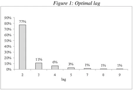
Figure 1: Optimal lag 12
Figure 2: β1 , β2 for factor 1,2 (n=10) 27
Figure 3: Volatility Estimation with Factor-BEKK (n=10) 28
Figure 4: β1 , β2 for factor 1,2 (n=15) 29
Figure 5: Volatility Estimation with Factor-BEKK (n=15) 30
Figure 6: β1 , β2 for factor 1,2 (n=20) 31
Figure 7: Volatility Estimation with Factor-BEKK (n=20) 32
Figure 8: β1 , β2 for factor 1,2 (n=25) 33
Figure 9: Volatility Estimation with Factor-BEKK (n=25) 34
Figure 10: Markowitz portfolio as n increases: 42
Figure 11: Frontiers of Markowitz portfolio as n increases: 43
Figure 12: Optimal weights n=25 for each stock 45
Figure 13: Optimal Selection weights n=25 for each stock for Sectors 46 Figure 14: Sample covariance UCG , PMI ( moving window of 100) 47 Figure 15:Estimated covariance UCG , PMI with BEKK 48
Figure 16: Variance-Covariance estimation 49
Figure 17: CVAR Minimum AIC lag distribution 50
Figure 18: CVAR rank distribution 51
Figure 19: CVAR p values F distribution 52
Figure 20: p values portmanteau distribution 53
Figure 21: p values portmanteau distribution 54
Figure 22: p values distribution 55
Figure 23: p values portmanteau distribution 56
Figure 24: p values portmanteau distribution 57
Figure 25: 95% approximate interval forecast 58
Figure 26:gaussian graphical model 66
Figure 27: Gaussian Finite Mixture 68
1. CVAR - BEKK - CC
1.1 IntroductionThe portfolio selection problem is discussed through the introduction of tree new types of models, called respectively CVAR-BEKK-CC, Factor-BEKK, multiple bi-dimensional CVAR-Factor-BEKK, that gradually increase the complexity of the solution while remaining computationally feasible.
The use of bivariate cointegrated vector autoregressive models and Baba-Engle-Kraft-Kroner models ( Engle et al. 1995), is proposed for the selection of a stock portfolio (Markowitz type portfolio) based on estimates of average returns on shares and the volatility of share prices. The model put forward envisages the use of explicative variables. This article employs the intrinsic value of shares as a variable, which will make it possible to take the theory of value into account. The model put forward is applied to a series of data regarding the prices of 150 shares traded on the Italian stock market.
The selection of a stock portfolio is broadly discussed in the literature, generally with reference to heteroskedastic regression models (Bollerslev
et al., 1994). The model used in the case of multiple time series is of the
vector autoregressive (VAR) type and rests on the predictability of the average return on shares (Brown and Reily, 2008, Hamilton, 1994).
In particular this paper suggests the use of cointegrated vector autoregressive models (CVAR) and Baba-Engle-Kraft-Kroner models (BEKK) for the selection of a stock portfolio. In other words, it addresses the problem of estimating average returns and the associated risk on the basis of the prices of a certain number of shares over time. This estimate is then used to identify the assets offering the best performance and hence constituting the best investments. While Campbell et al. (2003) proposes the use of a VAR(1) model, it is suggested here that use should be made of VEC models, which make it possible to take into account any cointegration between the series employed and the market trend as measured by means of the Thomson Reuters Datastream Global Equity Italy Index (Datastream 2008).
Moreover, while Bollerslev, Engle and Wooldridge (1988) employ diagonal vectorization (DVEC) models to estimate share volatility, the use
of a BEKK model, as proposed here, makes it possible to extend the estimation procedure based on DVEC models so as to take into account also the correlation between the volatility of the series and the volatility of the market trend.
The series considered regard the Italian stock market (BIT), and specifically the monthly figures for the top 150 shares in terms of capitalization, from 1 January 1975 to 31 August 2011.The estimation procedure proposed for portfolio selection involves two steps.
In the first step, a two-dimensional CVAR model is developed for all of the 150 shares considered in order to obtain an estimate of the average stock market return. A BEKK model is then applied to the series of residuals thus obtained in order to estimate the volatility of the series. The BEKK model appears particularly suitable because it does not entail the condition of normality for the accidental componentof the model (Hamilton, 1994).
The second step regards the selection of shares for inclusion in the portfolio. Only those identified as presenting positive average returns during the first phase are considered eligible. For the purpose of selecting the most suitable of these, a new endogenous variable is constructed as the product of two further elements, namely the price-to-earnings ratio (P/E) and earnings per share (EPS). This variable, which indicates the “intrinsic value” of the share in question, is not constructed for the entire set of 150 shares but only for those presenting positive average returns in the first phase, as it would be pointless in the case of negative returns.
The CVAR-BEKK model is applied once again to this new series in order to estimate the intrinsic value of the shares, and the top 10, (Evans and Archer, 1968), are selected for inclusion in the portfolio on the basis of the difference between this intrinsic value and the price estimated in the first phase (Brown and Reily, 2008).
A quadratic programming model is then employed to determine the quantities to be bought of each of the 10 shares selected.
It should be noted that the variable P/E EPS is estimated for each industrial sector (Nicholson, 1960).
2. The Cointegrated Vector
Autoregressive Models
2.1 Models description
A concise outline is now given of the phases involved in the selection of shares for inclusion in the portfolio as well as the quantity of shares to be bought for each type selected. The starting point is the series, regarding the average returns on the shares, and the average return of
the market , , . It should be noted in this
connection that the length of the series considered is not homogeneous because not all of the joint-stock companies are quoted as from the same point in time. This aspect involves further complications in the estimation procedure.
Step one : For each series, the model CVAR(p) is defined for the random
vector as:
with , is a
22
of the unknowncoefficients, and is the vector of errors such that
.
Model (1) can be rewritten as follows to take into account a possible cointegration of the variables considered:
where and (1) (2) (3) (4)
2.2 Specification , test and forecast
It has to be noticed that if
is singular, and
2,1, , 2,
'2 y y T
y are cointegrated (Johansen, 1995, Lutkepohl, 2007).
In specifying the CVAR model the lag order and the cointegration rank have to be determined. We start by determining a suitable lag length because, in choosing the lag order, the cointegration rank does not have to be known.
The AIC criterion is used to estimate the lag ˆp, with reference to model (1):
argmin min ln det~ : 0,1, , max
ˆ m p T mc m m C p u T m m (5)
where ~u
m is the maximum likelihood estimate (MLE) of u
m for aVAR(m) of type (1) with a sample of breadth T tk m and m values of initialization,with cT 8, pmax 10.
Notice that, while we have considered specifying the VAR order p, the criterion is also applicable for choosing the number of lagged differences in a VEC model (2) because p-1 lagged differences in a VEC correspond to a VAR order p (Lutkepohl, 2007).
In practice it is common to use statistical tests in specifying the cointegration rank. In this framework to ascertain the presence of cointegration in the model (2), the likelihood ratio test (LR) is used:
1 0 0 1 log r j j T r LR where: r0 rk
0,1 and j are the eigenvalues of the matrix2 1 11 01 1 00 10 2 1 11 S S S S S with
T p t t tu u p T S 1 ' 00 ˆ ˆ 1 ,
T p t t tv u p T S 1 ' 01 ˆ ˆ 1 ,
T p t t tv v p T S 1 ' 11 ˆ ˆ 1 . (6)The quantities uˆ , t vˆ are the residuals of the regressions oft yt and 1
t
y estimated by maximum likelihood (Johansen, 1995).
However, the asymptotic distribution of the LR statistic is nonstandard, in particular it is not a chi-squared distribution. In other words, the limiting distribution is a functional of a standard Wiener process. Percentage points of the asymptotic distribution, thus, critical values for the LR test can be generated considering multivariate random walks (Johansen et al., 1990).
Assessment of the presence of cointegration between the series by means of the LR test is followed by estimation of the parameters of the model.The result of the LR test is considered in deciding whether to adopt the model in form (1) or (2). In particular, if the test shows that the rank of matrix
is equal to 0 (hypothesis of stationarity of yt), then 0 and the method of maximum likelihood is applied directly to (2) in order to estimate the parameters 0, 1 and 1,,p1.If it instead transpires that the rank of
is equal to 1 (hypothesis ofcointegration of y1 and y2), then . In this case, it is necessary to
estimate model (2) in two stages. First, an MLE of is obtained by concentrating the log-likelihood with respect to . Second, this estimate is inserted into (2) in order to obtain the MLE of the other parameters (Johansen, 1995).
If rk
2, the method of maximum likelihoodis applied directly to (1) in order to obtain estimates of the parameters 0 , 1 and A1…, Ap.The portmanteau test is used to ascertain the presence of correlation of residuals, the generalized Lomnicki-Jarque-Bera test for the normality of residuals, and the ARCH test to determine heteroskedasticity
In order to forecast it is convenient in this framework to use the levels VAR representation. Therefore we consider the model type (1) with integrated and possibly cointegrated variables replacing the coefficients with their estimates as calculated before:
3. The BEKK model for
heteroskedasticity
3.1 BEKK model descriptionIn the event of the latter test revealing the presence of heteroskedasticity, the BEKK(1,1) model is used to estimate the conditional variance-covariance matrix
ut past
i j
t
i j nt
t 1 cov . , 1,,
which has the following structure:
The MLE of parameters ck,i,j at time t T is obtained by maximizing
the log-likelihood function:
3.2 ARCH-Test and Markowitz problem estimation
Once the parameters have been estimated, the Generalized Portmanteau test (Hosking, 1980) is applied to ascertain that the model BEKK(1,1) has effectively eliminated the ARCH effects in the residuals of the CVAR model:
(8)
m k p m k k m n n k g G G g Q 1 2 1 0 1 0 ' 1 2 ˆ ˆ ˆ ˆ ~ where pis the CVAR order, nT tmax, tmax max
ti,tj , gˆk vec
Gˆk ,L C L Gˆk T k ,
n k t k t t k n u u C 1 ' 1 ˆ ˆ ˆ , 1 0 ' ˆ C LL , m1 , ,10Step two: The estimates obtained in phase one are used to select the shares
for which positive average returns are predicted. For the shares thus selected and for each industrial sector (IS), the model CVAR(p)-BEKK(1,1) is estimated for the random vector
' , , ' , 2 , 1t, t ht, ISh t t y y P E EPS P E EPS y , where h1 , , H isthe index that identifies only the series with positive returns selected out of the initial 150.
On the basis of the
P E
EPS
h,T1 and Rh,T1 forecasts obtained in phase two, the shares are listed for each industrial sector in decreasing order with respect to the values of the difference between intrinsic value and expected price. The first n10 shares are thus selected to make up the portfolio.It should be stressed that the choice of n10is made on the basis of the assertion of Evans and Archer (1968) that this quantity is sufficient for diversification of portfolio choices. In actual fact, the number of shares selected will vary in further developments of this work.
In order to determine the quantities to be bought of each of the 10 shares selected, it is necessary to solve the Markowitz problem (Markowitz, 1952) by estimating the matrix of share volatility. To this end, let Vˆt be the estimator of the matrix nn of volatility V for t t T1, the elements of which are vi,j
t cov
Rt past
,i, j1,,nThe elements of are given by:
(10)
with
T t t j t j i t i n j i j i t T R R R R c C m ax max , , , , 1 , , ~ ~ ˆ ˆ , tmax max
ti, tj , bekk T T ii, 1 ˆ and ˆ11 i,T 1 in (8), i, j1,,n, n10.On the basis of (11), the solution of the following quadratic problem of Markovitz type, called global minimum variance portfolio, for the future
time T1 can be obtained with the approximation given by the dual
method (Goldfarb, 1983, Higham, 2002):
Vˆ : 1 1, 0
min ' T 1 ' RTo obtain a better diversification we have also to find the solution of the quadratic problem of Markovitz type (12) without the constraint
0, for the future time T1 using the explicit solution
1 1
1 ' 11 1 1 1 , ˆ ˆ ˆoptT VT VT Then we put to zero the i 0 and reprportionate the remaining i,
n i1 , , .
We omit the constraint of a fixed value for the expected return to eliminate the sensitiveness of allocation optimization to errors in predicted returns (Hlouskova et al., 2002).
In cases where the matrix VˆT1proves positive neither in (12) nor in
(13), we approximate it with the closest matrixin the sense of Frobenius possessing the same diagonal given by the elements estimated with the BEKK model.
(12)
4. CVAR - BEKK - CC Financial
application
4.1 Results
Application of the model proposed in this work to the monthly figures for the 150 BIT shares with the highest level of capitalization indicates the following results.
On the basis of the minimum AIC, the optimal lagpis 2–9 months. Figure
1 shows the empirical distribution of the lag. In particular, while the optimal lag is 2 months for 76% of the entire set of 150 shares it is 2 months for 90% of the shares in the portfolio and 1 month for the remaining 10%. This means that at least 2 months of observations are sufficient to predict the average returns on the vast majority of the shares considered, instead of a random walk model.
It was therefore decided to regard lag 9 as the maximum.
The results of the LR test for all of the shares considered, yields a degree of cointegration that proves equal to 2 for 91% of the 150 shares, 1 for 7% and 0 for the remaining 2%.
This means that in 7% of cases,when the rank of matrix
in (2) isequal to 1,use was made of the VEC model, which proves to be estimable (Johansen, 1995) and stationary, unlike the VAR model, which instead proves neither directly estimable nor stationary.
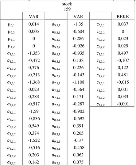
The coefficients of the model estimated in both steps of the procedure prove significant for almost all of the series considered. Table 1 shows, for example, the values of the coefficients estimated for models (1) and (8) for time series number 159.
Table 1: Parameters for models (1) and (8) – stock n°159 selected for the Portfolio.
stock
159
VAR VAR BEKK
0,1 0,014 a5,1,1 -1,35 c0,1,1 0,037 0,2 0,005 a5,2,1 -0,604 c0,2,1 0 1,1 0 a5,1,2 0,286 c0,1,2 0,023 1,2 0 a5,2,2 -0,026 c0,2,2 0,029 a1,1,1 -1,353 a6,1,1 -0,935 c1,1,1 0,497 a1,2,1 -0,472 a6,2,1 0,138 c1,2,1 -0,107 a1,1,2 0,376 a6,1,2 0,226 c1,1,2 0,122 a1,2,2 -0,213 a6,2,2 -0,143 c1,2,2 0,481 a2,1,1 -1,368 a7,1,1 -1,108 c2,1,1 -0,015 a2,2,1 0,023 a7,2,1 -0,564 c2,2,1 0,001 a2,1,2 0,283 a7,1,2 0,171 c2,1,2 0,033 a2,2,2 -0,517 a7,2,2 -0,287 c2,2,2 -0,001 a3,1,1 -1,59 a8,1,1 -0,902 a3,2,1 -0,836 a8,2,1 -0,692 a3,1,2 0,549 a8,1,2 0,391 a3,2,2 0,374 a8,2,2 0,265 a4,1,1 -1,522 a9,1,1 -0,37 a4,2,1 -0,516 a9,2,1 -0,458 a4,1,2 0,203 a9,1,2 0,062 a4,2,2 0,162 a9,2,2 0,075
The p value of F statistic is below 0.10 in 83% of cases and below 0.2 in 86%. The model thus proves 90% significant for nearly all of the series. Table 2 shows diagnostic tests for models (1) and (8). The results of the portmanteau Test on the residuals of the CVAR and BEKK models are given in Table 2 (here too, for brevity, they regard only the ten series selected for the portfolio). As regards the presence of ARCH effects in the residuals of the CVAR model (column 5 of Table 2: pAR), the test leads to the conclusion that the hypothesis of the presence of a heteroskedastic component in the model estimated at a confidence level of 99% cannot be ruled out for 60% of the shares chosen. The results of the Hosking test carried out in order to ascertain the presence of ARCH effects in the residuals of the BEKK model, which are shown in column 10 of Table 2 (pHq), lead to the conclusion that the hypothesis of the absence of any heteroskedastic component in the model is to be accepted in 90% of cases. In other words, it can be concluded that the combination of the CVAR and BEKK models picks up the heteroskedastic component and includesthe informationderived from the same in the procedure.
Column 9 (pH) of Table 2 shows the results of the portmanteau test carried out in order to ascertain the presence of autocorrelation of residuals in the BEKK model. They suggest that the hypothesis of autocorrelation can be ruled out and that the maximum lag considered is sufficient.
Table 2: Test statistics - stocks selected for the portfolio
Series R2.1 pFvalue pSC pAR pJB
4 0,114 0 0,187 0 0 34 0,085 0,006 0,717 0,475 0 63 0,078 0,08 0,785 0 0 130 0,014 0,894 0,347 0 0 49 0,052 0,007 0,664 0,002 0 109 0,041 0,736 0,502 0 0 159 0,725 0,02 0,049 0,458 0,847 85 0,179 0 0,2 0,056 0,001 54 0,12 0,01 0,838 0,131 0,025 60 0,113 0 0,423 0 0
Series pSK pKU pH pHq intervalYN
4 0 0 0,142 0,556 true 34 0,127 0 0,233 0,606 true 63 0,002 0 0,822 0,004 true 130 0,054 0 0,303 0,566 true 49 0,015 0 0,752 0,344 false 109 0 0 0,887 0,266 true 159 0,905 0,553 0,176 0,864 true 85 0,161 0 0,459 0,103 true 54 0,415 0,009 0,924 0,793 true 60 0,108 0 0,877 0,042 true
R2.1= goodness of fit stock equation1;
pFvalue = P(F>Foss|H0: Ai=0 ,i=1,…,p) zero coefficients of CVAR;
pSC =P (2>2oss | H0 : E(ut ut-i’) = 0, i=1,..,h>p ) autocorrelations in VAR residuals test;
pAR =P (2>2oss | H0 : no ARCH ) ARCH in CVAR residuals test;
pJB =P (2>2oss | H0 : normality ) CVAR normality test ;
pSK = P(2>2oss | H0 : E(ut3)=0 ) CVAR skewness test; pKU=P(2>2oss |H0 : E(ut
4
)=3 ) CVAR kurtosis test;
pH =P (2>2oss | H0 : no autocorrelations ) autocorrelations in BEKK residuals test;
pHq =P (2>2oss | H0 : no ARCH ) ARCH in BEKK residuals test;
A OLS-based CUSUM test for stability of the market index was also carried out, and the results suggest that the hypothesis of stability of the series over the period considered is acceptable.
The BEKK estimate of volatility for each share is between 0.001 and 0.01 for 93% of the series and never above 0.031.
It can be concluded in the light of this result that for most of the series considered, the estimated value of the share does not differ from its real value at a confidence level of 95%by more than 0.2.
In actual fact, the value at risk calculation put forward by J.P.Morgan (Longerstaey et al., 1995, Duffie et al., 1997). could be used in order to include the information deriving from the presence of correlation between the series considered and hence to assess the overall risk rather than the risk of the individual share.
Further confirmation of the adequacy of the CVAR-BEKK model with respect to the series observed was sought before selecting the shares to be included in the portfolio. Specifically, the confidence interval at the level of significance of 95% contains the actual value T +1 in 94 % of the series.
The CVAR-BEKK model can therefore be considered reliable for most of the series for the purposes of prediction.
The next step after verification of the suitability of the model was prediction of the prices of the shares as well as their intrinsic values. Table 3 shows the values predicted on the basis of model (7), once again restricted to the ten shares selected for the sake of brevity.
Table 3: Forecast return, volatility, intrinsic value, potential value – stocks included in portfolio
Series pf varf vinf indm vin_p
4 0,008 0,082 3,622 10 3,614 63 0,001 0,044 0,732 8 0,731 130 0,011 0,063 0,611 8 0,6 49 0,009 0,047 0,515 4 0,506 109 0,012 0,044 0,229 3 0,217 159 0,019 0,039 0,193 6 0,174 85 0,031 0,09 0,204 3 0,173 54 0,007 0,046 0,109 6 0,102 60 0,006 0,079 0,05 10 0,044 34 0,009 0,081 0,037 2 0,028 pf= forecasted return ; varf= forecasted volatility vinf= forecasted intrinsic value; indm= sector index;
On the basis of potentials, understood as the difference between share price and intrinsic value, the ten shares with the highest potential returns were then selected.
Two criteria of ranking were used, namely the partial criterion and the total criterion.
The former involves arranging the values of potential of all the shares considered in decreasing order for every industrial sector (Goodman and Peavy III, 1983) and selecting the first share in each.
In the latter, the values of potential of all the shares considered are arranged in decreasing order regardless of industrial sector and the first ten are chosen.
The use of the partial criterion is connected with the relationship between P/E and share performance manifested most strongly in each industrial sector. As Goodman and Peavy III write,“firms in the same
industry tend to cluster in the same relative P/E ranking, detected return differences between P/E groups may be attributable to industry performances rather than P/E level. This bias is eliminated by using P/E relative to its industry.”
The total criterion has the advantage that the selection is unconnected with the industrial sector of the share in question and therefore not necessarily influenced by the possibly negative trend of individual sectors. Its application thus means selection of the ten best shares in absolute terms (Nicholson, 1960).
The choice between these two criteria of ranking is obviously subjective in that it depends on the opinions of investors. This paper considers both, which evidently lead to the selection of different portfolios.
Table 4 lists the optimal allocations, i.e. the solutions of the problems of optimization (12) and (13); column 4 shows the results for the best portfolio. It has a monthly average return of 1.9%, a monthly standard
Table 4: portfolios weights, volatility, return, Sharpe Total Ranking Partial Ranking
Series w(i) prop. w(i) opt w(i) opt w(i) prop. Series
4 0,462 0 0 0,299 142 63 0 0,581 0 0 34 130 0 0 0 0,225 109 49 0,003 0 0 0 49 109 0,216 0 1 0,344 159 159 0,204 0 0 0,009 65 85 0 0 0 0 63 54 0 0 0 0,123 147 60 0,004 0,419 0 0 4 34 0,112 0 0 0 28 Return 0,011 0,003 0,019 0,011 Return St. Dev. 1,185 0,77 0,655 0,913 St. Dev. Sharpe 0,009 0,004 0,029 0,012 Sharpe 4.2 Comments
The selection of a share portfolio has historically constituted a complex problem that has no single solution but depends both on market conditions and on the information available to investors. In other words, the choice of shares to invest in must be based on objective criteria making it possible to assess risk and return without ignoring investors’ opinions. To this end, the paper suggests the use of a model for the analysis of multiple historical series with a view to the prediction of share return and associated risk but also taking the indications of the market into account at the same time in the specification of the model itself. Variables obtained as functions of P/E and EPS have thus been used together with the market index as regressors of the combined model (1) and (8).
The innovative choices in the construction of a portfolio selection model put forward here regard two distinct aspects. The first concerns transition from a model of the VAR (1) type for the prediction of a multiple historical series (Campbell, 2003) to one of the CVAR (p) type, which makes it
possible to take into consideration any cointegration of the series considered and therefore constitutes an improvement of the information available for estimation purposes. The subsequent use of a combinationof CVAR and BEKK models, which extends the results of Bollerslev, Engle and Wooldrige (2), makes it possible to consider also the temporally variable correlation between the volatility of the series and the volatility of the market index within the estimation procedure.
The second concerns the choice of criterion for the selection of shares,which is addressed here by seeking to insert a typical concept of finance such as intrinsic value into the primarily statistical context of the prediction of a multiple historical series. An intrinsic value estimated by means of the combined CVAR-BEKK model is used to obtain a “potential value” serving as a basis to rankthe different shares and then select the top ten.
The method put forward was applied to the seriesof 150 shares with highest capitalization quoted on the Italian stock exchange and led to the selection of 10 shares constituting a portfolio with an average monthly return of 1.9% and a risk of 0.655.
Comparison of the results of the CVAR-BEKK model put forward here and those obtained by means of models ofthe VAR (1) and DVEC type found in the literature was carried out on the basis of the values of log-likelihood of the models themselves. In other words, since one model could produce a higher value of return than another but nevertheless prove less reliable, it was decided to assess the models’ performance in terms of correspondence to the series observed. The log-likelihood of the CVAR-BEKK model always proves greater than that of the other models, thus indicating more accurate representation of the series observed and hence better predictions.
Further developments of the work will regard the study of “value at risk”, understood as assessment of the greatest loss possible, as well as identification of possible structural breaks of the individual series of share returns with a view to making the model more adaptable.
5. A Factor - BEKK model
5.1 IntroductionAs the CVAR-BEKK-CC model cannot explain the covariance between pairs of variables, the following Factor - BEKK model is used to explain the covariance through the help of two manifest factors, while retaining the computational feasibility of constant covariance.
The use of Factor Model combined with Baba-Engle-Kraft-Kroner (BEKK) model is proposed for the estimation of the volatility for stock portfolio (Markowitz type portfolio) The combined model uses esplicative variables as the instrisic value, which regards the value theory (Brown and Reily, 2008) and the market index (Sharpe 1970). The model put forward is applied to a subset of promising universe among the series of data regarding the prices of the best capitalized 150 shares traded on the Italian stock market (BIT) between 1 January 1975 and 31 August 2011.
The problem that arises in the stock portfolio selection framework is the estimation of the stock volatility, that is to say the estimation of the variance - covariance matrix of the stocks, as through the volatility it is possible to evaluate the risk of investment in the stocks (Markowitz 1952).
The diagonal elements and off - diagonal elements of the variance - covariance matrix are separately estimated: the former through BEKK models while the latter through a type 1 Factor model (Connor 1995).
In particular this paper suggests the use of BEKK model (Engle Kroner 1995) applied to the residuals of the bivariate cointegrated vector autoregressive models (CVAR) (Johansen 1995) for the compound stock values and the market index value (Pierini, Naccarato, 2012) to estimate the diagonal elements of the volatility matrix.
Per la stima degli elementi extra diagonali della matrice di volatilità si propone invece the use of a Factor model of type I (Connor G. 1995) with macroeconomic factor given by the market trend as measured by means of the Global Equity Italy Index (Datastream Global Equity Indices,
The Factor model utilization with respect to the use of sample covariance as an estimation of the off-diagonal elements of the volatility matrixhas the following pros: it gives the possibility to estimate with fewer parameters, that’s to say using 2n+n+4 parameters instead of n(n+1)/2 required otherwise. In doing so we obtain a more precise result because each parameter is estimted with error and with fewer parameters we accumulate less errors.
Moreover having fewer parameters to estimate is easier to update or add other stocks to the portfolio.
E’ comunque il caso di osservare che la stima della matrice di volatilità potrebbe risultare distorta poichè, se le stime degli elementi extradiagonali, derivano da un misspecified factor model, allora esse sono distorte (Ruppert, 2011).
La scelta di utilizzare due differenti procedure di stima per gli elementi della matrice di volatilità è dovuta a problemi di complessità computazionale; sarebbe in effetti auspicabile poter utilizzare il modello BEKK per la stima di tutti gli elementi della matrice di volatilità – poiché esso presenta caratteristiche migliori in termini di stime (Lutkpol new) di altri modelli già proposti in letteratura quali ad esempio modelli DVEC, ARCH, GARCH (Bollerslev, Engle et al. 1994). Tuttavia, al crescere del numero n delle azioni incluse nel portafoglio la stima del modello BEKK diviene computazionalmente non risolvibile (lutkepol new); da qui la nostra proposta di utilizzare la combinazione di modelli diversi per la stima della matrice di volatilità.
The series considered regard the Italian stock market (BIT), and specifically the monthly figures for the top 150 shares in terms of capitalization, from 1 January 1975 to 31 August 2011.
Before solving the volatility estimation problem, it is necessary to select the stocks to include in the portfolio and estimate the volatility of each stock during the time span considered. Starting with 150 stocks, in order to select the stocks to include in the portfolio, the procedure in two steps in Pierini, Naccarato, (2012) is uesd. It starts with the estimation of the market value of the stock through a CVAR(p) model (Johansen, 1995) and then the estimation – based itself on a CVAR(p) model – of its "intrisic value".
The intrinsic value is a new endogenous variable constructed as the product of two elements, namely the price-to-earnings ratio (P/E) and earnings per share (EPS). Si osservi che the “intrinsic value” of the share in question, is not constructed for the entire set of 150 shares but only for those presenting positive average returns in the first phase, as it would be pointless in the case of negative returns.
As far as the single volatilities are concerned – that are the diagonal elements of the volatility matrix – BEKK models are applied.
The n stocks included in the portfolio are then selected using a match between two estimated values, the intrinsic value and the market value. Only those identified as presenting positive average returns are considered eligible for the portfolio selection.
It is then possible to employ a quadratic programming model to determine the optimal n and the quantities to be bought of each of the n shares selected after estimating the volatility matrix.
5.2 BEKK model Estimates of the volatility matrix diagonal elements
The estimation of the diagonal elements of the volatility matrix is divided in three steps. It is estimated by applying the BEKK model to the CVAR(p) residuals of the stocks. However to estimate this model for the stocks it is necessary to have selected the n stocks to include in the portfolio. So in order to obtain the estimation of the diagonal elements of the volatility matrix in line with this methodology it is necessary to implement a two step procedure: firstly two CVAR(p) models are estimated, the first one applied on the returns and the second one applied on the intrinsic values. Then through a match between the obtained values, the n stocks to include in the portfolio are selected (Pierini, Naccarato, 2012). Lastly the BEKK model is applied to the CVAR(p) residuals to estimate the off-diagonal elements of the volatility matrix related to the n selected stocks on the basis of the match between the intrinsic values and returns.
To be noticed that as the selection of the stocks to include in the portfolio is done on the basis of the match between return and intrinsic value it is necessary that these two values are comparable.
So the transformation of the intrinsic value in a return intrinsic value is needed. This transformation is defined as the difference between the logarithm of the intrinsic value in the two successive times:
In altri termini, il modello CVAR è applicato al rendimento del valore intrinseco e non già al valore intrinseco.
(14) (15)
The CVAR(p) models are briefly described hereafter as a preliminary step for the estimation of the volatility the diagonal elements.
To estimate the time series of the return , the starting point is the K=150 series, regarding the returns Rk,t on the shares, and the average return of the
market RM,t , t=tk,…,T, k=1,…,K.
For each series the model CVAR(p) is considered for the random vector yt
=[y1,t , y2,t ]’=[Rk,t , RM,t ]’ as the equation (1).
To be noticed that the CVAR type model for the estimation of the unknown coefficients in the equation (1) is selected because it can detect the presence of cointegration or integration between the two components of the random vector yt, for the returns and for the instrisic values too, by considering its alternative reparametrization, called VEC form as the equation (2).
On the same 150 stocks, the bivariate time series of the intrinsic values and the intrinsic sector values is considered.
The sector is intended as the industrial sector to which each stock belogns.
For each series the model CVAR(p) like the equation (14) is considered for the random vector yt =[y1,t , y2,t ]’=[ (P/E)(EPS) h,t , (P/E)(EPS) IS(h),t ]’,
where h=1,…H is the index that identifies only the series with positive returns selected out of the initial 150.
On the basis of the (P/E)(EPS) h,T+1 and R h,T+1 forecasts obtained in
phase 2, the shares are listed in decreasing order with respect to the values of the difference between intrinsic value and expected price. The first
n{10,11,…,H} shares are thus selected to make up the portfolio.
To take into consideration the presence of heteroskedasticity (Pierini Naccarato 2012), the BEKK(1,1) model is used to estimate the conditional variance-covariance matrix of ut given in phase 1 of the
equation (1), t|t-1=cov(ut|past)=((i,j(t))i,j=1,…,n , which has the following
structure in the equation (8).
At the time t=T, the MLE (maximum likelihood estimations) of the parameters ck,i,j , k=0,1,2, i,j=1,2 are obtained maximixing the function
5.3 Factor model Estimates of the volatility matrix off-diagonal elements
Moreover the following two Factor model is applied
, i=1,…,n, t=1,…,T
where F1 is the market trend as measured by means of the Thomson
Reuters Datastream Global Equity Italy Index and F2 is the fundamental
factor given by the mean “intrinsic value”,k,i are parameters and i are
uncorrelated mean-zero random variables.
If we define , 0 =(0,1 ,…,0,n )T , Rt =(R1,t ,…,Rn,t )T , Ft =(F1,t , F2,t )T , =(1,t ,…,n,t )T
The model (4) can be reexpressed as
Rt = 0 + T Ft +t , t=1,…,T
Then, with j =(1,j , 2,j )T and F the 2 2 covariance matrix of Ft
We estimate the with the regression coefficients using (6) and F with
the sample covariance of the factors. By doing so we obtain an estimation of di,j .
In order to determine the quantities to be bought of each of the n shares selected, it to is necessary solve the Markowitz type problem (Markowitz 1952) by estimating the matrix of share volatility. To this end, let be the estimator of the matrix nn of volatility Vt for t=T+1, the elements of
which are vi,j(t)=cov(Rt|past), i,j=1,…,n .
We define the elements of by:
(16)
(17)
(18)
with
in the equation (2) i,j=1,…,n.
5.4 Results
Application of the model proposed in this work to the monthly figures for the 150 BIT shares with the highest level of capitalization indicates the following results.
In the following Table 5 we see the selected stocks with positive forecasted return: the number of this subset is H= 25
Table 5: Stocks selected for the Portfolio.
id pf varpf vinf indm vin_p var_vinf var_uf
28 0,04 0,117 0,052 2 0,012 0,236 0,353 113 0,034 0,096 -0,027 4 -0,061 0,162 0,258 85 0,031 0,09 0,204 3 0,173 0,336 0,426 44 0,029 0,085 -0,018 6 -0,047 0,82 0,905 117 0,028 0,063 -0,089 4 -0,117 0,182 0,245 38 0,022 0,071 -0,063 3 -0,085 0,326 0,397 159 0,019 0,039 0,193 6 0,174 0,221 0,26 109 0,012 0,044 0,229 3 0,217 0,237 0,281 130 0,011 0,063 0,611 8 0,6 0,876 0,939 45 0,01 0,103 -0,139 6 -0,149 0,305 0,408 147 0,01 0,047 -0,03 9 -0,04 0,087 0,134 34 0,009 0,081 0,037 2 0,028 3,682 3,763 49 0,009 0,047 0,515 4 0,506 0,865 0,912 4 0,008 0,082 0,943 10 0,935 1,385 1,467 32 0,007 0,081 -0,02 2 -0,027 1,979 2,06 54 0,007 0,046 0,109 6 0,102 0,32 0,366 14 0,006 0,062 -0,027 4 -0,033 0,134 0,196 60 0,006 0,079 0,05 10 0,044 0,114 0,193 57 0,005 0,089 -6,769 4 -6,774 0,103 0,192 156 0,004 0,069 -0,04 6 -0,044 0,341 0,41 7 0,002 0,038 0,019 10 0,017 0,055 0,093 104 0,002 0,095 -0,039 2 -0,041 0,309 0,404 63 0,001 0,044 0,732 8 0,731 1,9 1,944 65 0,001 0,063 -1,176 7 -1,177 1,617 1,68 142 0,001 0,049 0,027 1 0,026 0,212 0,261 column 1, called id, th ere is the identification number of the each stock;
column 2 , called pf, there is the forecasted return of each stock ( > 0); column 3 , called varpf, there is the forecasted return variance of each stock ; column 4 , called vinf, there is the forecasted intrinsic value of each stock ; column 5 , called indm, there is the industrial sector of each stock ;
column 6 , called vin_p, there is the difference between the intrinsic value and the return for each stock ;
column 7 , called var_vinf, there is the forecasted intrinsic value variance of each stock ;
In the following Figure 2 we see the betas for the two factors in a portfolio of the first n=10 stocks among the subset selected before .
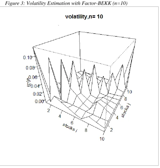
In the following Figure 3 we see the volatility matrix estimated with the Factor-BEKK model for a portfolio of the first n=10 stocks among the subset selected before :
In the following Figure 4 we see the betas for the two factors in a portfolio of the first n=15 stocks among the subset selected before:
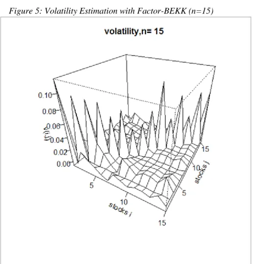
In the following Figure 5 we see the volatility matrix estimated with the Factor-BEKK model for a portfolio of the first n=15 stocks among the subset selected before :
In the following Figure 6 we see the betas for the two factors in a portfolio of the first n=20 stocks among the subset selected before:
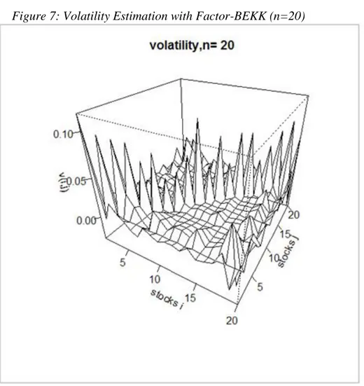
In the following Figure 7 we see the volatility matrix estimated with the Factor-BEKK model for a portfolio of the first n=20 stocks among the subset selected before :
In the following Figure 8 we see the betas for the two factors in a portfolio of the first n=25 stocks among the subset selected before:
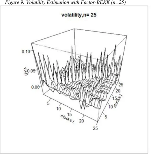
In the following Figure 9 we see the volatility matrix estimated with the Factor-BEKK model for a portfolio of the first n=25 stocks among the subset selected before :
Figure 9: Volatility Estimation with Factor-BEKK (n=25)
The Figure 2,4,6,8 show that the sensitivity of the stocks to the two factors changes with different number of stocks n in the portfolio. Sometimes the i,j may be near to zero showing no sensitivity of their relative stocks.
The Figure 3,5,7,9 show that increasing the number of stocks n in the portfolio has the effect of increasing also the covariance among the stocks (smaller or higher picks). Therefore it can give a considerable amount of decreasing in the overall portfolio variance.
To be notice that we start from n=10 as indicated in Evans Archer 1968.
5.5 Comments
The application of the Factor-BEKK model is an improvement of the multivariate estimation of the volatility matrix in (Pierini Naccarato 2012) because it gives an insight of the variability between the stocks through the macroeconomic market movements by using the market index factor. Moreover by using the intrinsic value factor it gives an insight also through
movements in the fundamentals P/E (Nicholson, S. F., 1960) and EPS which
make the intrinsic value.
Nevertheless this model maintains the dimension tractability of its predecessor avoiding the strong numerical intractability of a crude BEKK application to the overall n stocks (Lutkephol 2007) or the unreal semplicity of a sample covariance application to the overall n stocks.
6. Multiple bi-dimensional
BEKK model
6.1 Model description
The previous two models have the advantage of being computationally feasible while retaining a certain amount of power in the description of the real data involved. If the variances are regarded as time-dependent, however, then it is more plausible to regard the covariances as time-dependent too. This is supported by empirical results as well as the literature (Tsay 2010). Everything has its cost, however, and consideration also of time-varying covariances entails a considerable computational burden making BEKK infeasible for a dimension superior to 5 (Ding, Engle, 1994). A new method is put forward below to tackle this problem.
A combination of bi-dimensional BEKK models is proposed for estimation of the volatility matrix of the Markowitz stock portfolio. Each diagonal element of volatility is estimated by taking the variance given by a bi-dimensional BEKK model with stock i and the market index as variables. Each off-diagonal element of volatility is estimated by taking the covariance given by a bi-dimensional BEKK model with stocks i and j as variables.
The model is applied to a subset of promising universes among the series of data regarding the prices of the 150 shares with the highest market capitalization traded on the Italian stock exchange between 1 January 1975 and 31 August 2011. The volatility matrix of returns is required in order to select an optimal stock portfolio.
The diagonal and off-diagonal elements are estimated separately, as stated above, and the efficient frontier given by the solution of the estimated Markowitz problem is then simulated, thus providing the optimal number of stocks, fractions and returns in order to obtain the minimum-risk portfolio.
This approach gives a time-dependent overall estimation of the stock variances-covariances while resolving the computational burden through decomposition of the original problem without losing the strength of BEKK.
The application of a multiple bi-dimensional BEKK model is an improvement on the multivariate estimation of previous volatility-matrix models. Its purpose is to solve the infeasible problem of estimating the entire volatility matrix by breaking it down into multiple feasible bi-dimensional estimations, as in the other two previous models. The full strength of the BEKK model is used here in such a way as to make every estimation time-dependent. The estimation of the variances is not different from the previous time-dependent estimations, as each variance of stock i at time t depends on the variance of the market index at time t – 1, its own variance at time t - 1 and the covariance between the stock and the market index at time t - 1 (Ruey Tsay, 2010).
The market-index time series thus helps the forecast for each stock variance of interest.
The new idea is that the estimation of the covariance elements is now different from the previous time-independent ones in that each covariance between stock i and stock j at time t depends on the variance of stock i at time t - 1, the variance of stock j at time t - 1 and their covariance at time
t - 1.
In this way the covariance forecast for each pair of stock is guided by past correlation information.
The multiple bi-dimensional BEKK model is applied to the residuals of a bi-dimensional CVAR(p) model for each item in a set of n stocks. The CVAR(p) model also gives the predicted return for each stock.
In order to select the n most promising stocks, they are sorted in decreasing order with respect to their potential values. The potential value of a stock is the difference between its return and its compound intrinsic value, where the intrinsic value is the P/E times EPS.
The Markowitz portfolio is then solved and the dimension of the portfolio
n is increased by 1 each time to find the minimum-risk choice among the
best Markowitz portfolios.
The starting point taken in order to estimate the time series of market returns is the K=150 series with respect to the returns on shares Rk,t and the
average return of the market RM,t, t=tk,…,T, k=1,…,K.
For each series, the model CVAR(p) is considered for the random vector yt
=[y1,t, y2,t ]’=[Rk,t, RM,t ]’ as in equation (1).
The CVAR model makes it possible to deal with cases of the integration and cointegration of yt components whenever present.
For each series, as in equation (1), the model CVAR(p) is considered for the random vector yt =[y1,t, y2,t ]’=[ (P/E)(EPS) h,t, (P/E)(EPS) IS(h),t ]’,
where h=1,…H is the index that identifies only the series with positive returns selected out of the initial 150.
On the basis of the (P/E)(EPS) h,T+1 and R h,T+1 forecasts obtained in phase
2, the shares are listed in decreasing order with respect to the values of the difference between intrinsic value and expected price. The first
n{10,11,…,H} shares are thus selected to make up the portfolio.
BEKK1
In order to take into consideration the presence of variance
heteroskedasticity (Pierini Naccarato 2012), the BEKK(1,1) model is used
to estimate the conditional variance matrix of ut = [u1,t u2,t ]' = =[uk,t uM,t ]’
given in phase 1 of equation (1) for stock k and market index M, t|t-1=cov(ut|past)=((i,j(t))i,j=1,…,n,, which has the same structure as in equation
(8).
In order to take into consideration the presence of time-varying
autocorrelated disturbances (Pierini, Naccarato CFE 2013, Naccarato,
Pierini 2014) for each series previously selected, the model CVAR(p) is considered for the random vector yt =[y1,t, y2,t ]’=[Rk,t, Rs,t ]’, as in equation
(1). BEKK2
The BEKK(1,1) model is then used to estimate the conditional variance matrix of ut = [u1,t u2,t ]' = [uk,t us,t ]’ given by the residuals of equation (1)
for stock k and s, t|t-1=cov(ut|past)=((i,j(t))i,j=1,…,n,, which has the
following structure: (21)
At time t=T, the maximum likelihood estimations (MLE) of the parameters
dk,i,j, k=0,1,2, i,j=1,2 are by obtained maximizing the following function:
It should be noted that the (Q)ML estimator of the parameter vector
where the vec operator transforms a matrix into a vector by stacking its columns, , m = 0,1,2 , cannot be obtained analytically.
An iterative optimization algorithm is therefore required.
Use can be made of an algorithm of the Newton-Raphson type, which requires the first and second derivatives of (22), (Comte, Lieberman, 2003): and )
where A=(aik)i,k=1,...,n , tr(A) = a11+...+ ann , is the matrix
containing the first order derivatives of each element of with respect to , is the matrix containing the second order derivatives of
each element of with respect to .
(23)
(24)
(25) (22)
A BHHH algorithm type (Brandt, Hall, Hall, Hausman, 1974) can be implemeted for the s-step as :
where is the step length.
Moreover the (Q)ML estimator , as obtained above, is almost certainly consistent and
where , , even if the distribution of ut
is not normal as long as some regularity conditions are met (Comte, Lieberman, 2003).
Finally, the procedure of estimation in two steps – where the parameters of the CVAR are estimated in the first and the residuals of this model are then used to estimate the BEKK parameters in the second – is justified because the estimators of CVAR end BEKK are asymptotically independent (Lutkepohl 2007).
In order to determine the quantities to be bought of each of the n shares selected, it is necessary to solve the Markowitz problem iteratively with no shorting (Markowitz 1952) by estimating the matrix of share volatility:
where , .
To this end, let be the estimator of the matrix nn of volatility Vt for t=T+1, the elements of which are vi,j(t)=cov(Rt|past), i,j=1,…,n .
The elements of are defined as follows:
(29) (28) (26) (27)
where are the estimates obtained respectively from
equations (1) and (2) with i,j=1,...,n:
Whenever is not a positive definite n × n matrix, the Goldfarb-Idnani (1983) numerically stable dual method for finding the nearest positive definite n × n matrix to is used to ensure positive portfolio risk
.
6.2. Multiple 2D- BEKK Results
Application of the model put forward here to the monthly figures for the 150 BIT shares with the highest level of capitalization gives the following results. The selected stocks with positive predicted returns are a subset of maximal dimension nmax = 25.
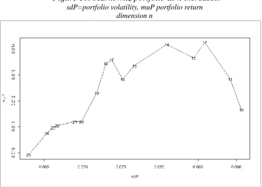
Figure 10 shows the volatility and the return obtained by solving the
Markowitz optimization problem for variation in the expected return Rp;T+1
and the dimension n of the portfolio (n = 10, 11,…, nmax), where nmax = 25
is the maximum number of shares with positive predicted returns. The portfolio risk tends to decrease as n increases.
A dimension n=12 would give the maximum return 0.01423 but with a high risk of 0.0859.
Figure 10: Markowitz portfolio as n increases: sdP=portfolio volatility, muP portfolio return
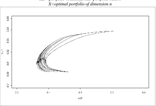
Figure 11 shows the efficient frontiers obtained by solving the Markowitz
optimization problem for variation in the expected return Rp;T+1 and the
dimension n of the portfolio (n = 10, 11,…, nmax), where nmax = 25 is the
maximum number of shares with positive predicted returns.
Figure 11: Frontiers of Markowitz portfolio as n increases: sdP=portfolio volatility, muP portfolio return
X=optimal portfolio of dimension n
In overall terms, the portfolio risk tends to decrease as n increases. The optimal risk from a risk-averse standpoint (i.e. the least of all those calculated) corresponds to n = 25. This point is located closer to the origin of the axes and marked in figure 2 as X. This portfolio has a monthly average return of 0.00993, a monthly standard deviation of 0.0630 and a Sharpe index 0.15771. A portfolio is therefore selected of n = 25 shares with the optimal allocations shown in Table 6.
Table 6: Optimal weights n=25 id op. w 4 0,06 7 0,03 14 0,02 28 0,04 32 0,01 34 0,05 38 0,03 44 0,02 45 0,06 49 0,05 54 0 57 0,04 60 0,02 63 0,06 65 0,08 85 0,04 104 0,03 109 0,02 113 0,04 117 0,06 130 0,04 142 0,07 147 0,03 156 0,03 159 0,09
The selection for the portfolio of n = 25 shares with the optimal allocations is also shown in Figure 12. It can be seen that the allocation is quite diversified over the stocks.
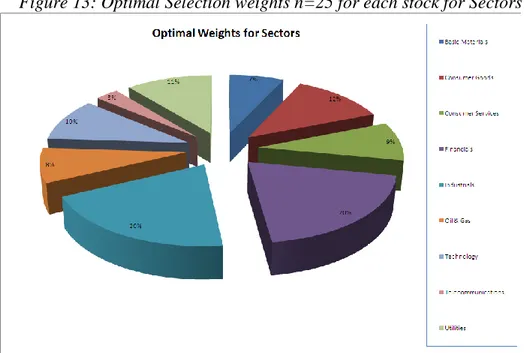
The optimal selection for the portfolio made up of n = 25 shares for each industrial sector is shown in Figure 13. It can be seen that the allocation is quite diversified over the stocks with a prevalence for the industrial (20%) and financial (20%) sectors.
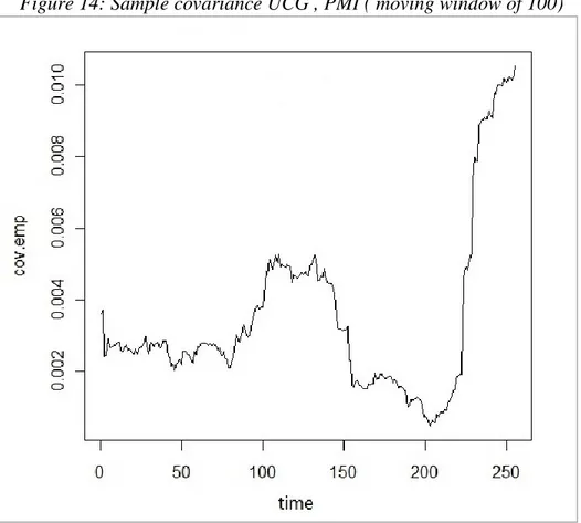
The empirical evidence of time-varying covariance can be seen, for example, by considering two stocks as in figures 14 and 15. Figure 14 shows the sample covariance between UCG and PMI using a moving window of 100 observations. This smoothing suggests that covariance changes over time. Figure 15 shows the same covariance estimated with a BEKK model so that it varies each time.
The estimation with equation (30), which is used to calculate the previous portfolio, is shown in Figure 16.
Figure 16: Variance-Covariance estimation with multiple bi-dimensional BEKK at T+1|T
Some elements of the estimated covariance are larger than others and comparable with the variance. Let us call this subset As. Most of the
covariances are instead lower than the ones in As and negligible with
respect to the variance.
This suggests that it would be possible to separate the statistical analysis of the shares belonging to set As from the analysis of those belonging to the
On the basis of minimum AIC, the optimal CVAR lag is 2–9 months. There is thus empirical evidence of market inefficiency, as the past has information to explain the future. Figure 17 shows the empirical distribution of the optimal lags. As prediction is the primary objective, AIC is chosen as the lag criterion because it is asymptotically equivalent to the FPE (Final Prediction Error).
The results of the LR test for all of the shares considered yield a degree of cointegration between 0 and 2. The 9% of instable time series (integrated and cointegrated) are taken into due consideration. Figure 18 shows the empirical distribution of the matrix, defined in (4), in ranks.
Figure 19 shows the empirical distribution of the p values of F statistics
for testing H0 : ah,ij = 0 in equation (1). This is equivalent to verifying the
hypothesis that the model estimated does not exist.
It can be seen that H0 is rejected at a confidence level of 90% in 83% of the
time series. The CVAR model is therefore adequate for most of the cases.
Figure 20 shows the empirical distribution of the p value of the
portmanteau statistics for testing H0: no correlation in the CVAR residuals.
It can be seen that H0 is rejected at a confidence level of 90% in 6% of the
time series. The CVAR model is therefore adequate for most of the cases even though some lags could be added. This is not done here because the prevailing criterion for lag selection is AIC.
Figure 20: p values portmanteau distribution for no correlation in CVAR res
Figure 21 shows the empirical distribution of the p values of the
portmanteau statistics for testing H0: no ARCH in the CVAR residuals.
It can be seen that H0 is rejected at a confidence level of 90% for 79% of
the time series. The CVAR residuals are therefore affected with ARCH effects in the majority of cases and GARCH modelling is required because it can represent this effects.
Figure 21: p values portmanteau distribution for no ARCH in CVAR res