A
A
l
l
m
m
a
a
M
M
a
a
t
t
e
e
r
r
S
S
t
t
u
u
d
d
i
i
o
o
r
r
u
u
m
m
–
–
U
U
n
n
i
i
v
v
e
e
r
r
s
s
i
i
t
t
à
à
d
d
i
i
B
B
o
o
l
l
o
o
g
g
n
n
a
a
DOTTORATO DI RICERCA IN
SCIENZE BIOTECNOLOGICHE E FARMACEUTICHE
Ciclo XXXII
Settore Concorsuale: 03/D1
Settore Scientifico Disciplinare: CHIM/08
Dynamic Docking, Path Analysis and Free Energy Computation in
Protein-Ligand Binding
Presentata da:
Martina Bertazzo
Coordinatore Dottorato
Supervisore
Prof. Maria Laura Bolognesi
Prof. Andrea Cavalli
Co-supervisori
Prof. Matteo Masetti
Dr. Sergio Decherchi
TABLE OF CONTENTS
ABSTRACT ... 3
LIST OF ACRONYMS ... 4
1 INTRODUCTION ... 6
1.1 Molecular Recognition as the basis for drug action ... 6
1.2 Thermodynamics and kinetics of biological complexes ... 7
1.3 Protein-ligand binding models ... 10
1.4 Experimental and computational strategies to characterize protein-ligand interactions ... 12
1.4.1 Experimental methods ... 12
1.4.2 Computational methods ... 14
1.5 Summary of the contribution ... 17
2 THEORETICAL AND METHODOLOGICAL BACKGROUNDS ... 19
2.1 Molecular Dynamics (MD) simulations ... 19
2.2 Estimation of MD-derived observables ... 22
2.3 Enhanced sampling methods ... 24
2.3.1 Potential-Scaled MD (sMD) ... 25
2.3.2 Well-tempered metadynamics ... 26
2.3.3 Steered MD (SMD) ... 29
2.3.4 The MD-Binding Approach ... 29
2.4 Path Collective Variables (PCVs) ... 31
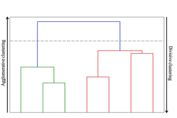
2.5 Analysis of multiple conformations: Cluster Analysis ... 32
2.5.1 Hierarchical algorithms ... 33
2.5.2 Non-hierarchical algorithms ... 34
2.6 Applications of MD-based techniques to the study of the protein-ligand binding process 35 2.6.1 Plain MD ... 35
2.6.2 Enhanced sampling methods relying on CVs ... 37
2.6.3 Enhanced sampling methods based on tempering ... 38
3 ORIGINAL CONTRIBUTIONS ... 40
3.1 Fully Flexible Docking via Reaction-Coordinate-Independent Molecular Dynamics Simulations ... 40
3.1.1 Introduction ... 40
3.1.2 Methods ... 42
3.1.3 Results and discussion ... 49
3.2 Predicting residence time and drug unbinding pathway through sMD ... 60
3.2.1 Introduction ... 60
3.2.2 Methods ... 61
3.2.3 Results and Discussion ... 65
3.2.4 Conclusions ... 71
3.3 A Semi-automatic protocol to identify path collective variables to perform well-tempered metadynamics and to compute the protein-ligand binding potential of mean force. ... 73
3.3.1 Introduction ... 73
3.3.2 Methods ... 75
3.3.3 Results and Discussion ... 80
3.3.4 Conclusion ... 86
4 CONCLUSIONS ... 88
ABSTRACT
Comprehending how drugs interact with biological macromolecules to form a complex with consequent biological response is particularly relevant in drug design to guide a rational design of new active compounds. The establishment and the duration of the protein-ligand binding complex is principally determined by thermodynamics and kinetics of the dynamical process of molecular recognition. Thus, an accurate characterization of the free energy governing the formation of the protein-ligand complex is of fundamental importance to deeply understand each contribution to the establishment of the molecular complex.
Experimental biophysical techniques, such as ITC (Isothermal Titration Calorimetry), NMR (Nuclear Magnetic Resonance) and SPR (Surface Plasmon Resonance) proved to be efficient in characterizing both thermodynamics and kinetics of protein-ligand binding. However, a detailed description of the whole binding process on a mechanistic level, with the characterization of all the metastable states is not possible since only a quantitative estimation is allowed.
Conversely, from the computational point of view, plain molecular dynamics (MD), which has been increasingly considered as the method of choice to investigate the entire dynamic process upon complex formation and to predict the associated thermodynamic and kinetic observables, cannot be applied in a routinely drug discovery pipeline because of the high computational cost. In particular, in order to reconstruct a reliable free energy associated to the protein-ligand binding process, all the configurational space has to be extensively sampled, taking longer than the time commonly available in a usual campaign of drug discovery.
In this context, this PhD thesis wants to address specific aspects of the protein-ligand binding process. In particular, it will deal with dynamic docking, thermodynamics and kinetics of protein-ligand binding by devising respectively three different computational protocols. We developed a dynamic docking protocol based on potential-scaled (sMD) simulations, in which both the protein and the ligand are let completely flexible in order to predict the protein-ligand binding pose within a reasonable computational time (Chapter 3.1). Then, we further investigated the applicability of sMD in describing the kinetic behavior of a series of drug-like molecules and we devised a fully automated method to analyze the unbinding trajectories, detecting common features (Chapter 3.2). Finally, we develop a semi-automated protocol based on path collective variables (PCVs) combined with well-tempered metadynamics (well-tempered MetaD) to estimate free energies along a binding path (Chapter 3.3).
LIST OF ACRONYMS
ITC Isothermal Titration Calorimetry
SPR Surface Plasmon Resonance
NMR Nuclear Magnetic Resonance
HTS High-Throughput Screening
MD Molecular Dynamics
FES Free-Energy Surface
MM-PBSA Molecular Mechanics Poisson-Boltzmann Surface Area MM-GBSA Molecular Mechanics Generalized-Born Surface Area
GPU Graphical Processor Unit
GSK3! Glycogen Synthase Kinase 3! HSP90" Heat Shock Protein 90" PBC Periodic Boundary Conditions
PME Particle-Mesh Ewald
CV Collective Variable
US Umbrella Sampling
SMD Steered Molecular Dynamics
MetaD Metadynamics
REMD Replica Exchange Molecular Dynamics aMD Accelerated Molecular Dynamics McMD Multicanonical Molecular Dynamics
PT Parallel Tempering
sMD Potential-scaled Molecular Dynamics
PES Potential Energy Surface
PCVs Path Collective Variables
MSD Mean Square Deviation
RMSD Root Mean Square Deviation
MSM Markov State Model
HTMD High Throughput Molecular Dynamics SuMD Supervised Molecular Dynamics BS-MetaD Bias-Exchange Metadynamics
RMD Reconnaissance Metadynamics
SITMD Selective Integrated-Tempering-Sampling Molecular Dynamics
ENM Elastic Network Model
COM Center of Mass
RMSIP Root Mean Square Inner Product PCA Principal Component Analysis MDS MultiDimensional Scaling method
1 INTRODUCTION
1.1 Molecular Recognition as the basis for drug action
Molecular recognition refers to process in which macromolecules, such as proteins, bind small molecules through noncovalent interactions to form a binary complex. This mechanism, which regulates several biological processes and plays a central role in disease and homeostasis, deals with two important attributes that describe the protein-ligand interaction: specificity and affinity. Specificity is related to the capability of proteins to prefer those binding partners that are highly specific than those that are less specific, while affinity is related to the strength of the protein-ligand complex.1 Molecular recognition is thus of fundamental importance in the development of drugs,
especially during the lead optimization phase, since affinity and specificity determine whether a molecule has the potential to become a drug.
Traditionally, the activity of drug-like molecules has been expressed in terms of the equilibrium dissociation constant, #$, or by half-maximal inhibitory concentration %&'(, both often performed under closed in vitro conditions. #$ measured in vitro, can be, in certain specific cases, directly correlated to the in vivo efficacy of a ligand. However, most frequently, this relation does not directly hold, particularly when the in vivo efficacy is mostly determined by the duration of the pharmacological effect. Indeed, sometimes the time for which the biological target is occupied by a ligand, commonly referred to as drug target residence time, )*, that corresponds to the inverse of the dissociation rate constant ()* = 1/./00), could be more appropriate to describe the efficacy than binding affinity.2 This aspect recently propelled the need of including the kinetic profiles,
expressed in terms of the association rate constant, ./1, and the dissociation rate constant, ./00, in drug discovery programs, especially during the drug optimization phase.2 It is therefore of the
utmost importance for a deep knowledge of drug action that the processes responsible for the protein-ligand interactions are well characterized mechanistically and quantitatively in energetic terms.3
In the first section of this thesis, a brief introduction about the physiochemical mechanisms that control the protein-ligand association is given. In particular, a general description of the most important concepts related to the molecular recognition, such as binding kinetics and thermodynamics, free-energy, entropy-enthalpy compensation are provided. Then a description of the three existing theories, the lock-and-key, induced fit and conformational selection theories, describing the protein-ligand binding are introduced in order to underline the fundamental importance of considering protein flexibility to study biological processes. The final part of this Introduction section is dedicated to experimental and computational methods applied to investigate the protein-ligand binding mechanism.
1.2 Thermodynamics and kinetics of biological complexes
The first attempt to provide a systematic description for the temperature dependence of equilibrium constants of a reaction was proposed in 1889 by Svante Arrhenius. In particular, according to Arrhenius equation, the rate constant k of a chemical reaction can be calculated as:
. = 34589:67 (1)
Where ;< is the activation energy of the process, = is the temperature, and the pre-exponential term A, is a constant that describes the number of times two molecules collide, and it is characteristic for each chemical reaction since it is a function of the collision radius between two interacting particles and the reduced mass of the system. Despite the Arrhenius equation has been used to determine activation energies for chemical reactions, it can be exploited only to the kinetics of gas reactions in which the transformation to form the product does not involve any intermediate. The transition state theory, as coincidentally formulated in 1935 by Henry Eyring, Meredith Gwynne Evans and Michael Polanyi, was developed to describe more accurately the kinetic behavior of the chemical systems. According to this theory, it is possible to gain insight into rates of reactions by investigating the activated complexes, the so-called transition states. In situations of chemical equilibrium between reactants and activated transition state complexes, the former could convert into products and the kinetic theory could be applied to obtain the rate of this conversion.
According to transition state theory applied to a fully solvated protein-ligand complex, along a single binding path, the dynamics of the transition depends only on the slowest step involved (the one associated to the highest energy). However, reaching an accurate description of the potential energy surface (PES) of the system, especially for the transition states, is far from trivial and, as a result, the absolute reaction rate constants are difficult to obtain.4
It is important to underline that the binding or unbinding kinetics is not defined by only one transition state but different pathways are possible, with different transition states associated, can contribute to the observable ./1 and ./00 values, so understand which transition state, among all the transition pathways, represents the limiting one could become tricky.5 Despite these
considerations, transition state theory is of fundamental importance in describing protein-ligand interactions and in determining thermodynamics quantities such as Gibbs energy of activation, enthalpy and entropy (Figure 1).
In a first order reaction, the noncovalent association between a protein ? and a ligand @ in solution to form the biomolecular complex ?@ can be described as the equilibrium:
? + @ ./1
Where ./1 and ./00 are the kinetics rate constants that account for both the binding and unbinding reaction. The units of ./1 and ./00 are M-1 s-1 and s-1, respectively. At equilibrium this two-state
mechanism is perfectly symmetrical. In particular the binding reaction is balanced by the reverse unbinding reaction according to:
./1[?][@] = ./00[?@] (3)
Where the equilibrium concentration of all the species involved in the reaction are represented by the square brackets. The binding affinity is then described by the dissociation constant #$ (in unit of M):
#$ =[F][G]
[FG] (4)
In this situation, #$ corresponds to the ligand concentration at which half of the receptor binding sites are occupied. #$ is directly associated to the free energy difference between the bound and unbound states, ∆I$. According to equation (3) and equation (4), the thermodynamics constant #$ is linked to the kinetics constants ./1, ./00, as follow:
#$ =KLMM
KLN (5)
Therefore, it is interesting to understand how complexes with the same affinity could have, at least in principle, very different transition states. Indeed, varying the transition state decreases or increases both kinetic rates without altering the energy difference between both the bound and unbound states. This because the rate constants ./1 and ./00 depend on the transition state along the binding pathway that separates the bound and unbound states:
./1//00 =K9O
P 4
∆QLN/LMM‡
S: (6)
According to the above equation, the kinetic constants, ./1, ./00, are proportional to the exponential of the energies of activation of the respective transitions state, ∆I/1//00‡ , through a pre-exponential factor that combines the Boltzmann’s constant .T, the Planck’s constant ℎ , and the absolute temperature =.
Figure 1. Simplified free-energy profile of the protein-ligand complex ?@ formation between a protein ? and a ligand @. TS represents the transition state. The thermodynamics of binding is quantified by the free energy difference between both the bound and unbound states (∆GW), and the kinetics is determined by the
dissociation and the association rate constants, kXY, ./00. These quantities are related to the free-energy
differences between minima and the transition state TS, ∆I/00‡ and ∆I/1‡ , respectively.
As already discussed, much consideration has been given to the impact of including kinetics information in the optimization phase of the drug discovery process, since models based both on kinetic constants and binding affinity can be more reliable.
The protein-ligand binding process in a solvent is an example of thermodynamic system so it is possible to describe the driving forces that dictate the association of the two entities using the laws of thermodynamics. In particular, as any spontaneous process, the establishment of the protein-ligand complex ?@ occurs only when the change in Gibbs free energy, ∆I$, of the system is negative, once the system reaches an equilibrium state at constant pressure and temperature. At the steady state, ∆I$ can also be defined as the variation of the unbound to the bound state of two state functions of the system: enthalpy (Z) and entropy ([) with the following equation:
∆I$= ∆Z − =∆[ (7)
For a binding process, the binding enthalpy, ∆Z, reflects the energy change of the system when the ligand binds to the protein, resulting from the formation of noncovalent interactions between them.6
Change in binding enthalpy is a global propriety of the entire system. This means that the change upon biding involves also contributions from the solvent, in particular the formation of new interactions between the ligand and the protein coincides with the disruption of interactions between ligand and solvent, protein and solvent and a new solvent reorganization near the complex
surface.1 Entropy is a measure of the disorder or randomness of the overall system (including the
ligand, protein and surrounding solvent). ∆[ is a global thermodynamic observable of a system which is positive when the overall degree of freedom of the system increase and, on the contrary, the negative sign indicates decrease in degrees of freedom of the system. The binding entropy, ∆[, is determined by:
∆[ = ∆[]/^_+ ∆[`/10+ ∆[*/a (8)
Where ∆[]/^_ reflects the solvent entropy change in the accessible surface area of the protein and ligand upon complexation; ∆[`/10 represents changes in the conformational entropy reflecting the changes in the conformational degree of freedom of protein and ligand upon binding and ∆[*/a represents the loss of rotational-translational degrees of freedom of protein and ligand upon binding.7
As introduced before, the sign and magnitude of ∆I$ are determined by the variation of entropy and enthalpy. Thus, ∆H and ∆[ can be considered as the driving forces for the protein-ligand binding event. In particular, negative enthalpy change, which is associated with the establishment of new noncovalent interactions between association partners, is accompanied by a negative entropy change caused by the loss of degrees of freedom of protein and ligand. This phenomenon, where variation of ∆I$ is caused by mutual variation in ∆Z and ∆[, is called the entropy-enthalpy compensation.8 Different mechanisms can contribute to the entropy-enthalpy compensation,
including the structural and thermodynamic proprieties of the solvent, the protein flexibility and the molecular structure of the ligand.
1.3 Protein-ligand binding models
The mechanisms underlying biomolecular recognition have been deeply investigated, in order to understand these processes and define new active compounds in a drug discovery context.9–13 Three
different models have been introduced for ligand recognition, the “lock-and-key”,9 “induced fit”11
and “conformational selection”13–16 (Figure 2).
According to the lock-and-key model (Figure 2A), the protein and the ligand are considered rigid and they possess specific complementary shapes that match exactly into one another, like a key into a lock, with almost no change in protein conformation. The binding event is based on the grounds that desolvation of the protein and the ligand during the process leads to changes in entropy contribution. In particular, the collision between the protein and the ligand causes a complete displacement of the water network surrounding the protein and ligand interaction interfaces,
causing a positive enthalpy change, while the release of water increases the solvent entropy. According to this model, that considers the protein as rigid, there is no change in conformational entropy. Therefore, the solvent entropy should be large enough to compensate the positive enthalpy change due to the desolvation process and also the negative entropy caused by the loss of rotational and translational motions of the ligand. The lock-and-key model fails to explain the experimental evidence that a protein is also able to bind to a ligand even in the case where their initial shapes do not fit perfectly.
Conversely, the induced fit model, considering the flexibility of both the interacting binding partners, the ligand and the protein binding site, is able to provide a plausible explanation (Figure 2B). According to induced fit model, during the interaction with the ligand, the protein undergoes a conformational change only in the binding site, neglecting major conformational changes that could involve the whole protein structure. The absence of the initial perfect surface complementary between protein and ligand results in multiple tentative collisions to establish favorable contacts (negative enthalpy change), that should be strong enough to provide the encounter complex enough strength so that induced fit takes place in a reasonable time.1 Particularly, in order to maintain the
stability of the protein-ligand complex, the negative enthalpy change contribution, resulting from the establishment of interactions between protein and ligand should be greater than the sum of the positive enthalpy change resulting from the disruption of the interaction with the solvent, the negative entropy change resulting from reducing the conformational freedoms of the interacting surfaces, ∆[`/10, and the rotational-translational degrees of freedom of the binding partners, ∆[*/a.
Furthermore, the lock-and-key and induced fit models consider the protein, under given experimental conditions, as a single and stable conformation. Instead, most proteins are intrinsically dynamic, and the conformational selection model considers their flexibility (Figure 2C). In accordance with this model, the native state of a protein exists as an ensemble of different conformations, all coexisting in equilibrium with different population distributions, and the ligand binds the one that is more selectively altering the equilibrium toward this state. It is difficult for the conformational selection model to understand which state of the system, entropy or enthalpy, contributes the most to the lowering of the system’s free energy. In particular, it seems like the selective binding of the ligand to a specific conformational state of the protein is dominated by the solvent entropy gain due to the desolvation effect (as occurs in lock-and-key-model), while, the following conformational adjustments of the protein is dominated by the system enthalpy decrease due to the formation of newly interactions between interacting partners.
It is important to underline that, because these three conceptual models for biomolecular recognition have been observed experimentally, they may exist simultaneously or in a sequential
manner, and also that even more complicated mechanisms than those presented here may be possible.17
Figure 2. Schematic illustrations of the three different protein-ligand binding models: the lock-and-key (A),
the induced fit (B), and the conformational selection (C). The protein is represented in blue while the ligand is represented in orange.
1.4 Experimental and computational strategies to characterize
protein-ligand interactions
Several experimental and computational techniques could be used to investigate different aspects of protein-ligand binding. In this regard, isothermal titration calorimetry (ITC), nuclear magnetic resonance (NMR) and surface plasmon resonance (SPR) are briefly introduced in the first part of this paragraph as experimental methods to characterize protein-ligand binding while, in the second part, molecular docking and binding free energy calculations are discussed as theoretical approaches.
1.4.1 Experimental methods
ITC is a biophysical technique that allows a direct estimation of the heat exchange during the complex formation at constant temperature; this is probably the gold standard in determining the energies driving the binding process.18 ITC allows simultaneous determination of binding affinity
change ∆[ in one single experiment. A typical ITC experiment is a three steps procedure. In the first step, the ligand is titrated into a solution containing the biomolecular target of interest. The second step consists in measuring the heat absorbed or released that is associated with the binding event. In particular, the temperature imbalance between the reference and sample cells, due to protein-ligand binding event, is measured and compensated by modulating the feedback power applied to the cell heater. During the last step the primary ITC data, that are the power applied to the sample cell as a function of time, are processed and fit to obtain the binding curve representing the heat of reaction per injection as a function of the ratio of the total ligand concentration to the protein concentration. Finally fitting the binding curve, the binding constant #d = 1/#$, the binding enthalpy ∆Z, and the stoichiometry of the binding event n are obtained. Consequently, knowing the binding constant, the standard Gibbs free energy ∆GW, the binding entropy ∆[ can be derived. The heat exchange revealed by ITC is the total heat effect in the sample cell consequent the ligand addition, including the heat adsorbed or released during the binding event as well as the heat effects due to the dilution of the ligand and protein, the mixing of two different solutions, the different temperature between the sample and references cells, and so on. Therefore, evaluating the heat change due to the contribution of binding only is far from trivial.
NMR spectroscopy is a particularly efficient method exploited to get information about protein-ligand interactions at atomic resolution.19 Several NMR spectroscopy approaches exist to study
protein-ligand complex which can be categorized into two general group: protein observed or ligand observed techniques.
In protein observed methods, a spectrum of protein is obtained, and the ligand is titrated, thus providing information about residues of the protein directly involved in the interaction with the ligand. Conversely, in ligand observed techniques, the spectrum of ligand is obtained, and the protein is added. The overall NMR spectra depends on the lifetime of the protein-ligand complex which is given by the residence time ()*). In particular, for strong complexes the lifetime of the protein-ligand complex is much longer than the difference in chemical shifts between the signals obtained for the unbound and bound form, thus two separate NMR signals are obtained. On the contrary, when weak complexes are involved, the lifetime of the complex is too short to observe the two signals independently and a single NMR signal is obtained.
SPR spectroscopy20 is a popular technique used for the estimation of association and dissociation
rate constants during protein-ligand binding or unbinding events. SPR is an optical-based method that assesses the change in the refractive index near the sensor surface. It is a label-free technique, which is advantageous in comparison with the radioligand binding assays that have been previously used for the biochemical characterization of the formation of specific drug-target complexes. In the
most widespread configuration, the sensor surface is a thin gold film on a glass support, which is positioned on the bottom of the flow cell through which an aqueous solution flow.
The receptor molecules are immobilized on the sensor surface and the ligand (analyte in SPR terminology), is injected into the aqueous solution. As the analyte binds to the immobilized receptor, an increase in the refractive index is observed. Once all the binding sites are occupied, a running buffer without analyte is injected through the flow cell to let the ligand molecules dissociate from the target protein. As the analyte dissociates, a decrease in the refractive index is measured. The time-dependent resonance unit (RU) curve is processed and fitted to determine the association and dissociation rates, ./1 and ./00. The equilibrium dissociation constant #$ is quantified by fitting the resonance unit sinusoidal curve as a function of the analyte concentration. Moreover, the binding enthalpy can be estimated by van’t Hoff analysis.21 It is important to note that by
immobilizing the protein, the conformational and roto-translational entropies may be affected impacting on the evaluation of the association rate constants.
1.4.2 Computational methods
Even if experimental techniques can investigate thermodynamic profiles for a ligand-protein complex, the operations for measuring the binding affinity are laborious, time-consuming, and expensive. In a modern rational drug design campaign, to find a set of lead molecules, high-throughput screening (HTS) of a large library of hundreds or thousands of samples is involved. Thus, it is hardly feasible or even possible to achieve this goal using only experimental methods. The opportunity to predict completely in silico ligand binding modes and to investigate binding processes to identify and optimize new lead candidates motivates the Scientific Community to put great efforts in developing new computational techniques. Molecular docking can predict, for instance, very quickly which ligand fits best into the binding pocket of the protein target and assess the binding affinity of the complex. More accurate predictions of binding affinity could be obtained through molecular dynamics simulations, which take in account all thermodynamically relevant phenomena such as the protein flexibility and explicit inclusion of the solvent.
1.4.2.1 Molecular Docking
Molecular docking is a well-established computational strategy for predicting in silico the binding modes and affinities of molecular recognition events.22 Thank to the constant growth of available
protein structures and to the improvement in computational resources, molecular docking has been proven to be an important methodology for drug discovery campaigns.23 This procedure allows to
compounds that are likely to have an action against the target of interest, thus saving time and costs. However, this computational speed occurs at the cost of accuracy, especially when protein rearrangements are required upon ligand binding.24,25 Indeed, protein flexibility is not treated
extensively; additionally water molecules, which can be crucial for reproducing the specific protein-ligand complexes, are very difficult to treat explicitly. However, thanks to the methodology advances several different software have been developed to include explicit water molecules into docking and virtual screening studies26 such as: GRID,27 HINT,28 Superstar,29 JAWM,30
WaterMap,31 Water PMF32 and Water FLAP.33 Therefore, an accurate evaluation of the
thermodynamic and kinetic quantities is not allowed.
At the time of the earliest implementations of molecular docking, around 1982 when the first molecular docking was reported by Kunts et al.22, both ligand and protein were treated as rigid
bodies but, nowadays, full flexibility of the ligand and partial flexibility of the receptor are implemented by almost all docking programs.34
A typical docking algorithm consists of two main components: the search algorithm and the scoring function. The former component, which can be either stochastic or deterministic, is responsible for searching through different ligand conformations and orientations (poses) within a given target receptor’s binding site. As already introduced, the early docking implementations dealt with a unique rigid conformation of the protein due to limited computational resources. However, proteins are intrinsically dynamic and, most of times, there is a mutual adaption between protein and ligand in order to maximize favorable interactions upon binding.35 In principle, according to
the more recent interpretation of molecular recognition models, the degrees of freedom of protein and ligand should be sampled simultaneously, but this is still too computational demanding, so a number of different strategies were developed to provide a solution.
These can be split into two main groups: single-structure methods or ensemble methods. Single-structure methods are related to the induced-fit model in which only the binding pocket is perturbed by on-the-fly local changes after ligand binding conformational search. Alternatively, in ensemble methods, an ensemble of previously generated conformations is exploited in a series of independent docking procedures mimicking the conformational selection model. Anyway, information provided by induced-fit approaches and multiple protein conformations is difficult to manage and it must be properly used to be effectively exploited.36,37
Scoring functions are approximate mathematical methods used to assess the binding affinity (generally through estimating the strength of noncovalent interactions) in a protein ligand complex. In order to reduce the algorithm’s complexity, since many different physical interactions (including those with the solvent) as well as the entropic effects need to be considered in a reliable estimation of binding free energy, a number of simplifications are introduced at the cost of accuracy.38 The
general classes: the force-field-based, the empirical-based and the knowledge-based (also known as statistical potentials) scoring functions.
In the force-field-based approaches, binding affinities are estimated by using functional forms and parameters, defined as force-fields, derived from experiments and quantum mechanical calculations. In order to reduce the complexity, usually only the enthalpic contribution, mostly due to the strengths of intramolecular noncovalent interactions between interacting partners, is taken into account. The desolvation energies of the ligand and of the protein are sometimes re-estimated using implicit (or continuum) solvation methods such as Molecular Mechanics Poisson-Boltzmann surface area (MM-PBSA)39,40 and the generalized-Born surface area version (MM-GBSA).41,42
Empirical scoring functions are based on the parametrization of different types of interactions, usually via regression methods, as favorable or unfavorable energy terms contributions to the binding affinity.43 The knowledge-based scoring functions assume that statistical observations of
intramolecular close contacts between protein and ligand that occur more frequently than those expected by a random distribution are likely to be energetically favorable and therefore contribute favorably to binding affinity. Thus, these contacts are used to derive the statistical potentials. All these three scoring functions, known as classical scoring functions, assume an additive functional form to represent the linear relationship between the binding affinity and those features that describe the protein-ligand complex. By contrast, Machine learning scoring functions, which use pattern recognition algorithms to discriminate mathematical relationships between empirical observations, do not make suppositions about the form of the functional.44,45
In summary, molecular docking represents a valid method to identify crystallographic binding modes and to select new promising compounds from entire libraries of molecules, especially when protein flexibility does not play a fundamental role in the binding process. Instead, when large rearrangements are involved in the protein-ligand binding process, molecular docking suffers from severe limitations. Moreover, molecular docking does not provide the necessary accuracy to calculate a reliable estimation of binding free energy and it cannot be used to estimate kinetics quantities. In principle, all these problems could be overwhelm by molecular dynamics (MD) simulations and related methods.46
1.4.2.2 Molecular Dynamics (MD) simulations
MD simulations describe the physical evolution of the system in time solving Newton’s equations of motion, immersed in a thermic bath, where forces between the interacting particles and their potential energies are calculated using molecular mechanics force fields. During the last decade, thanks to the advent of faster architectures and development of more specific computation algorithms, MD simulations have become a valid alternative to traditional molecular docking in
drug design since the exploration of the entire protein-ligand process at full atomistic level is allowed, in principle. Moreover, the possibility to investigate the entire protein-ligand binding process could shed light on metastable states sampled by the ligand, protein conformational rearrangements during or consecutive the ligand binding, alternative binding sites, and also the contribution of the water during binding.47 Additionally, provided that simulations of the binding
process are long enough to observe the entire mechanism, from the drug completely solvated water (unbound state) to the formation of protein-ligand complex (bound state), thermodynamics and kinetics observables can be accurately evaluated through the estimation of the free-energy surface (FES) as described in the following section of this thesis (2.2 Estimation of MD-derived observables).46,48 However, multiple binding events have to be observed along the simulation in
order to collect an adequate statistics to correctly calculate thermodynamics and kinetic quantities. This usually require milliseconds simulations making the process too computationally expensive to be routinely used instead of traditional molecular docking methods especially in the first part, when novel compounds have to identified or during the hit-to-lead optimization.
In order to reduce the computational cost required, a number of different enhanced sampling techniques have been developed during the last years. These methods accelerate MD simulations, increasing the probability of observing binding process, by applying biasing forces or altering the potential energy function. Thanks to these techniques combined with the ever-increasing computational power, MD simulations are gaining everyday more attention in drug discovery process, replacing the standard molecular docking with the new concept commonly referred as “dynamic docking”.25,48
1.5 Summary of the contribution
MD has been increasingly considered as a promising computational technique to study protein ligand-binding since the entire mechanism can be investigated and, in principle, the associated thermodynamic and kinetic observables can be estimated. However, due to the significant computational effort involved, the direct application of plain MD to study protein-ligand binding is often not possible or highly inefficient, at least from a drug discovery perspective.
In this contribution, we explored possible different protocols, depending on the specific issue to address, based on enhanced sampling MD simulations to gain insights into thermodynamics and kinetics associated to the protein-ligand binding process.
In particular, three different aspects of protein-ligand binding are considered: prediction of ligand binding mode into the target binding site, estimation of residence time for a congeneric series of
compounds binding to the same biological target and the computation of the FES of the entire mechanism of ligand binding.
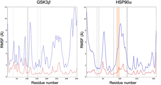
In the first application, a semi-automated protocol based on an enhanced sampling technique, the scaled-potential MD (sMD), is developed in order to predict protein-ligand binding poses. This protocol was validated on its ability to reproduce the crystal binding poses of a set of five different compounds binding two relevant pharmacological targets (the Glycogen Synthase Kinase 3!, GSK3!, and the N-terminal domain of Heat Shock Protein 90", HSP90").
As for the second test case, we exploited sMD to perform a series of unbinding simulations of a series of congeneric compounds, inhibitors of HSP90", in order to prioritize them according to their average computational exit times. Moreover, we devised a protocol based on dimensionality reduction and clustering analysis to qualitatively compare pathway followed by the ligands during unbinding simulations.
Finally, in the last test case, we devised a semi-automated strategy to compute a guess path along with the FES of the whole protein-ligand binding process. To achieve this, we took advantage of a machine learning algorithm introduced by Ferrarotti et al,49 known as principal path to identify a
binding path from pre-existing MD-binding simulations. In addition, we reconstructed the FES exploiting the well-known well-tempered Metadynamics algorithm.
2 THEORETICAL AND METHODOLOGICAL
BACKGROUNDS
During the last decades, MD simulations have been optimized properly in order to capture accurately the full protein-ligand binding process in agreement with experimental results. This is due to increasing computer power, the advent of graphical processor unit (GPU) architectures, and MD software that can efficiently run on these innovative infrastructures.50 As already discussed in
Introduction, in pioneering studies by Buch et al.51 , Shan et al.52 and Dror et al.53, several
spontaneous protein-ligand binding events reproducing the complexes resolved by X-ray crystallography, were observed. However, as it was previously discussed, several different trajectories are needed to obtain adequate statistics and to sample exhaustively the conformational space. This makes the whole process computationally demanding and not frequently affordable, especially in fast-paced drug discovery, when MD simulations are used for kinetic prediction of ligands with long residence time.46 However, powerful alternatives to the plain MD simulations
have been developed in order to accelerate the observations of rare events on affordable timescales.54 Most of these approaches, usually referred as “enhanced sampling methods”, can
provide also the statistical weights of the sampled configuration, allowing the reconstruction of the thermodynamics of the system consistent with the one obtained by a plain MD simulation. In this section, we provide some theoretical background on methods and combination thereof we employed to study protein-ligand binding process and related thermodynamics and kinetics proprieties of biologically relevant systems.
2.1 Molecular Dynamics (MD) simulations
Molecular dynamics, MD, is a computational technique aimed at studying the time-dependent evolution of a molecular system, under the action of the forces generated by a potential that provides opportune approximations of the physics and chemistry under investigation. This is obtained by solving the second-order differential equations represented by Newton’s second law:
ef()) = ifjf()) = −kl(m(a))km
n(a) (9)
Where ef()) is the force acting on ith atom of mass mp, at time t. jf()) is the acceleration and x(t) represents a configuration of the system described by three-dimensional coordinates of the N interacting atoms at time t. Commonly, in computational drug discovery, molecule’s atoms are treated as a sphere particles according to molecular mechanics principle. This is possible through
contribution to the system dynamics is associated to nuclear motions, which are considerably heavier than electrons in term of mass. This allows to average out the electronic contribution in Schr edinger’s wave function equation that describes the system. The result is that an empirical potential energy function is introduced q(r())) that represents the Force Field (FF):
q = ∑ Kt,n u (vf− v/) u+ ∑ Kw,n u ("f− "(,f) u+ ∑ x∑ ln8 u y1 + cos (}fK∙ •fK − Ä K a/*]f/1] f <1Å^Ç] f d/1$] f •(,fK)ÉÑ + ∑ ÖfÜáà*â,nä *näã åu − à*â,nä *näã ç é + ∑ ènèä êëíâíì*nä î<f*] f,Ü î<f*] f,Ü (10)
The FF accounts for bonded and non-bonded contributions. In equation (10)the first three terms represent bonded terms describing variations in potential energies as a function of bond stretching, bending and torsion among atoms directly involved in bonding relationships. Bond stretching and bending, represented by summation over bond lengths (l) and angles (") respectively, are both described by harmonic potentials with reference values v( and "( and force constants of .^ and .ï. Torsions of dihedral angles are described by a cosine series of M terms, and other parameters are additionally considered that take in account the periodicity. In particular, describes the multiplicity for the kth term of the series, •(,fK is the corresponding phase angle, and qfK is the energy barrier. Non-bonded terms describe forces acting among atoms that are not directly bound and consist of van der Waals and Coulomb interactions (fourth and fifth term in equation (10) respectively). These forces vary with the inverse power of the distance between considered atoms ñfÜ. In particular, van der Waals interactions are generally described by a 12-6 Lennard-Jones potential, where εpò defines the depth of the energy well, whereas ñ(,fÜ is the minimum energy distance that equals the sum of the van der Waals radii of the two interacting atoms considered. The last term in equation (10) describes the electrostatic energy that is defined by the Coulomb potential. ôf and ôÜ are the partial charges of the pair of considered atoms, Ö( is the permittivity of free space and, finally, Ö* is the dielectric constant (1 in vacuum). The empirical determination of reference values for bond lengths, angles, dihedral together with the different degree of accuracy used to describe the non-bonded interactions limits the applicability of the FF. However, multiple FF with constantly increasing accuracy are now available, so one can always take in account the FF best fitting to the specific considered molecular system. In a normal MD simulation, given a certain FF and potential q(r())), it is possible to derive the acceleration over the atoms with respect to positions x at time t. Even if a classical FF speeds up calculations compared to quantum mechanics (QM), equation (10) still it requires integration over time. Thus, to simulate biological macromolecules it is necessary to split the integration of the equation of motion into discrete time intervals, known as time-steps (δt), where forces are assumed to be constant. As an example of an integrator, the velocity-Verlet is one of the most widely adopted algorithm in MD simulations. The Velocity-Verlet integrator calculates positions at time () + ú)) through the following equation:
rf() + ú)) = rf()) + ùf())ú) +å
ujf()) (11)
Where rf()), ùf()) are the coordinates and velocities at time t respectively, accelerations jf()) are calculated taking the first derivative of the potential energy with respect to positions with opposite sign as shown in equation (11). Velocities are then calculated according to equation:
ùf() + ú)) = ùf()) +åu[jf()) + jf() + ú))]ú) (12)
The accuracy of integrators heavily depends on the value of the chosen time-step, that must be chosen small enough to track the dynamics of the system.
Only a “small” δt guarantees reliable forces over time and consequently, continuous trajectories. Ideally, the value of the time-step should be comparable to the time scale of the fastest motion among those that are being studied. For example, stretching and bending of bonds involving hydrogen atoms are subjected to very fast motions so a correct value of time-step should be 0.1 fs. This time step is very small and a strategy to increase it is to constrain the fastest degrees of freedom subjected to very fast motions thanks to ad-hoc algorithms (i.e., stretching and bending of bonds involving the hydrogen atoms).56 In this way, it is possible to neglect these motions and thus
consider a time-step 10 times larger, heavily reducing the computational cost. Other strategies are possible: for example, implementing a protocol to repartition the hydrogens mass over adjacently bound heavy atoms, allowing a time step of 4 fs.57,58 Alternatively these masses are not considered
at all and replaced with virtual sites without mass,58 whose positions are updated relatively to heavy
atoms at each step.
An important aspect that any numerical integrator must satisfy when used in an MD simulation, is the preservation of the energy conservation law. In particular, the integrator must keep the Hamiltonian of the system constant, given by the sum of the potential and kinetic energy. According to the following equation:
Z(r, û) = q(r) + #(û) (13)
the Hamiltonian Z(r, û) provides the total energy of the system and depends upon coordinates (x) and momenta (p). From these considerations, because the macroscopic variables that define the statistical NVE ensemble are considered constant, MD naturally follows the motion of a microscopic isolated system, without exchanging energy with the surroundings. Most of the MD simulations are performed within the canonical ensemble, where the number of particles (N), volume (V) and temperature (T) are conserved, or within the isothermal-isobaric ensemble, where N, V and pressure (P) are conserved. Constant temperature is maintained through a thermostat.59
immersed in a thermostatic bath. Constant pressure is controlled by the so-called barostat algorithms,60,61 that is by opportunely scaling the system volume. In order to limit the finite size
effects due to the use of a simulation box, periodic boundary conditions (PBC) are also commonly used in MD simulations. With the employment of PBC conditions, the system is placed in a unit cell that is replicated in different directions resulting in a periodic lattice of identical subunits. In this way, molecules of the system that are close to the edge interact with the atoms of the neighboring box. In order to limit the computational cost of the non-bonded terms calculations, a spherical cut-off with a radius usually at least 11 Angstrom has to be used. In particular, the forces are divided into short- and long-range contributions depending on the distance value as below or over the above mentioned threshold.
The long-ranged electrostatic interactions, because they decay as ñ5å, are usually calculated over the a lattice through particle-mesh Ewald (PME) method.62 While short-range electrostatics is
computed in the real-space, a grid-based approach is used in the reciprocal space to calculate long-range electrostatic taking advantage of fast Fourier transform.62
Generally, MD simulation setup consists of three important steps: minimization, equilibration and production. During the minimization step, the initial structure of the system is relaxed to the nearest local minimum (potential energy).61 During the equilibration step, the system is brought at
physiological temperature and pressure conditions. The initial velocities are assigned to the atoms according to a Maxwell-Boltzmann probability distribution at the desired temperature. This step should be gentle enough to avoid artifacts in the protein structure, so generally, it is a good practice to run few steps in the NVT ensemble, in the first heating steps. Once the temperature reaches an acceptable value (e.g. 300 K), a switch to the NPT ensemble is necessary to relax the system. By use of these methods, MD simulations on systems of relevant pharmaceutical interest can be performed from the microsecond to millisecond time scale in order to observe events such as drug binding to its target and to estimate the kinetics and free energy associated with protein ligand binding.
2.2 Estimation of MD-derived observables
According to statistical mechanics principles it is possible to quantitively estimate important thermodynamics observables computed from MD runs, such as internal energy, pressure and heat capacity. Among these, as already discussed in the Introduction, the key thermodynamic quantity in drug discovery is the protein-ligand standard binding free energy,46 ∆I
$°, defined as the free energy difference between the unbound and bound states.63 ∆I
$° can be directly compared to the experimental dissociation constant KW through the following equation:
∆I$° = .
T=v} †°£¢°§ (14)
Where &° is a constant defining the standard concentration (1 M by convention) that makes the argument of the logarithm dimensionless. 64 Because the standard binding free energy depends on
the dissociation equilibrium constant #$ and the reference value of &°, this conventional concentration must be properly considered to compare computational free-energy estimation with experimental data.64 Together with other quantities related to entropy, free-energy is the
thermodynamic observable whose estimation suffers the most from the limitations and underlying approximations of the sampling. Because of the probability of visiting microstates in the canonical ensemble is proportional to the Boltzmann factor according to:
û(r) ∝ 45l(m)/(K9O) (15)
It is evident that thigh-in-energy configurations are much less frequently sampled than low-energy states. In addition, if barriers larger than .T= units need to be crossed, the sampling of the configurational space will be severely limited, which is a prerequisite to achieve reliable energy estimate. For this reason, moving across different states, separated by significant free-energy barriers, can be viewed as a rare event relative to the time scales accessible to plain MD simulations. Equation (15) can be expressed as a function of the probability rate between bound and unbound states as:
∆I$° = −.
T=v} †îî¶LßN¢(m)
ßN¶LßN¢(m)§ + .T=v} †
£¶L®
£° § (16)
Where ûd/©1$(r) and û©1d/©1$(r) are the probability of finding the protein in the bound or unbound states, respectively. The second term is a correction term to obtain the standard binding free energy. This term considers as well as the reference concentration of the standard state, C° and the concentration of the interacting species included in the simulation box &d/m. The MD approach, together with Monte Carlo methods, are the most accepted techniques to generate a Boltzmann distributed set of configurations, finding application in studying biomolecular systems. However, assessing free energy as a probability ratio according to equation (16) is far from trivial, since many re-crossing events between the bound and unbound states, separated by energy barriers larger than .T= units, are required to achieve proper statistical confidence. For plain MD simulation, this is even harder since it is already pretty rare to observe a single binding event in a reasonable computational time.
As it was already widely discussed in Introduction chapter, the main advantage of MD-based methods is the possibility of characterizing the mechanistic steps of the entire protein-ligand binding process.
In particular, provided that adequate sampling is obtained, kinetic observables such as the association and dissociation constants (./1 and ./00) can also be determined by using equations (5-6).
During the last decade, kinetics received increasing attention in the drug discovery field, following the perspective article of Copeland published in 20062 where the concept of residence time define
as the reciprocal of the ./00 is thoroughly discussed:
)* = Kå
LMM (17)
His discussion starts from the evidence that t´ is related to the in vivo biological effects triggered by the ligand. In other words, the efficiency of a drug is explicated only when the drug is bound to its physiological target, whose cellular function is consequently modified.65,66 Thus, from a
pharmaceutically standpoint, accurately predicting the )* can be more important than the determining the equilibrium constant to predict the final in vivo drug efficacy. Therefore, optimizing )* via rational design is of fundamental importance for computational drug discovery. However, plain MD simulations are not appropriate to recover transition rates for drugs; this is due to the long timescales involved in the dissociation of protein-ligand complexes, which can last from millisecond to minutes or more.
2.3 Enhanced sampling methods
Thanks to improvements in hardware and software, it is now possible to perform long MD simulations able to observe in detail the full protein-ligand binding process, at least in some cases. However, due to the huge time scale needed to adequately sample the configurational space involving the binding event, it is not possible to routinely exploit plain MD in the drug discovery process, making the plain MD binding more like academic exercise. Indeed, most of the times, simulating the whole process of ligand binding to its target requires the exploration of a large number of degrees of freedom, and also the ligand may spend a lot of time in irrelevant regions in the bulk solvent before finding the way to the binding site. As result, the system gets trapped in a local minimum of the FES, without being able to overcome the energy barrier and explore other regions, including that associate with the absolute minimum corresponding to the protein-ligand crystallographic complex.
To overcome this limitation, a number of strategies, the so-called “enhanced sampling methods”, have been developed.46,67 As suggested by the name, they improve the exploration of the
configurational space.67 Broadly speaking, these methods usually fall in two general categories. On
one side, one has methods that rely on collective variables (CVs) biasing. The main advantage of using these strategies is that the sampling is enhanced toward the event of interest by biasing the MD simulations along chosen CVs, that are functions of atomic coordinates. Among these methods, the most well-known are umbrella sampling68 (US), steered MD69 (SMD), and metadynamics70
(MetaD). On the other side, one has tempering methods, in which sampling is enhanced along all of the degrees of freedom of the system. Replica exchange MD71 (REMD), accelerated MD72
(aMD), multicanonical MD73 (McMD), Parallel tempering (PT),71 and potential-scaled MD74,75
(sMD) belong to this second class.
In this work, we took advantage of both classes of enhanced sampling methods so, in the following, a brief description of the theory behind the employed techniques is provided.
2.3.1 Potential-Scaled MD (sMD)
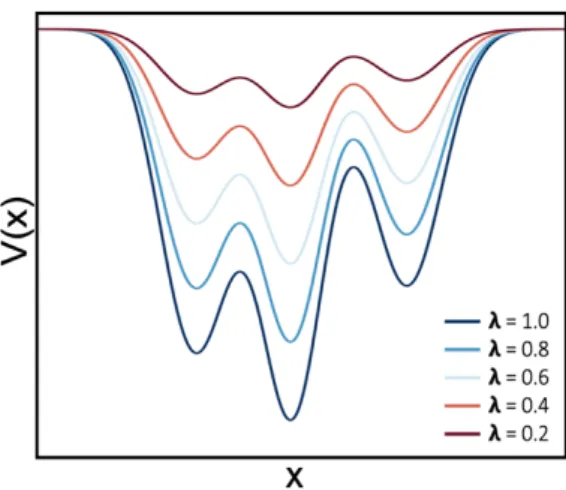
sMD belongs to the non-CV based class of methods.74,75 In this method the PES of the system is
scaled by a factor λ that belongs to the interval (0,1]. When
λ equals to 1, then the PES corresponds to that obtained from a plain MD. As one goes to lower values of λ, approaching the 0 value, the energy profile is increasingly smoothed. In Figure 3 it is depicted the effect of λ on the PES. As a result, the energy barriers between different states are lowered and thus transitions between them are facilitated. This behavior is the analogous to sampling at high temperatures. Under sMD conditions, the canonical probability distribution for a given state of the system is modified to:
û∗(r) = 45Æl(m)/K9O (18)
Where V(x) is the potential energy along a reaction coordinate r, .T is the Boltzmann constant and
Figure 3. Effects of the scaling factor in the PES of the system. As more aggressive λ values are applied, the potential energy profile increasingly smoothed.
In this implementation from Sinko et al., a population-based reweighting scheme was proposed to reconstruct the canonical distribution of populations:
û(r) = û∗(r)å/Æ (19)
In principle it is possible to consider other reweighting schemes, including for instance an energy term. However, it was shown that the population-based strategy is more accurate, as energetic terms are subjected to larger energy fluctuations that introduce large errors.74
2.3.2 Well-tempered metadynamics
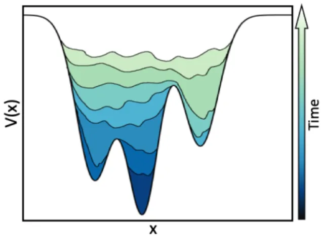
MetaD is a well-known enhanced sampling method for studying rare events.70 In MetaD the
sampling is enhanced by adding a history-dependent bias potential constructed by depositing Gaussian kernels on selected degrees of freedom or CVs, that essentially describe slow degrees of freedom of the system. The bias potential added through MetaD is expressed by means of the following function: q±(≤(r), )) = ≥ ∑ exp ∂−à](m)5]†m∑a ∏π§ã∫ uªº∫ Ω a a∏ æ ø Q,uøQ (20)
where, w is the height of the Gaussian distributions, ¿] is the width of the Gaussian potentials, and ¡± is the time frequency at which Gaussian potentials are deposited along the CVs of a microscopic coordinate x of the system, s(x). These three parameters determine the accuracy and efficiency of
the free energy reconstruction. If the Gaussians are large, the FES will be explored at a fast pace, but the reconstructed profile will be affected by large errors. Instead, if the Gaussian are small or are deposited infrequently, the reconstruction will be more accurate, but it will take a longer time. The bias potential fills the minima in the FES, allowing the system to efficiently explore the space defined by the CVs. Figure 5 reports an example how MetaD acts with a one-dimensional bias potential.
Figure 5. Pictorial representation of the MetaD method. The bias is gradually deposited at increasing time
intervals τ along a r. Assuming that a simulation starts from the deepest basin, the gradual filling due to Gaussian deposition allows crossing the barriers and visiting the second deepest basin. The less profound basin is sampled after the other two basins are filled and the system is able to cross the barrier separating from them. Once all of the relevant minima have been visited, the system is free to sample along the entire reaction coordinate. At this point, minus the total bias accumulated gives the free energy.
In MetaD it is assumed that for a sufficiently long simulation, the system is able to freely diffuse in the CV space. One can reconstruct the free energy √(≤(r)) in such CV space as:
lim
a→«q±(≤(r), )) = −√∑≤(r)π + & (21)
Where C is an irrelevant additive constant. The main drawbacks of using MetaD are related to assessing the convergence of the simulation and choosing the CVs to bias.76 As for the first one,
once all the basins are visited, and while the simulation keeps running, the bias continues being deposited. This has the effect of overfilling the underlying FES and encouraging the system to visit high-energy regions of the CVs space. Thus, for a reliable FES estimate, the simulation should be stopped as soon as the system starts diffusing in the CVs space. A solution to this problem is provided by well-tempered MetaD.77 While in standard MetaD Gaussians of constant height w are
time. As a result, the overfilling mentioned above is less pronounced. Now, the Gaussian height becomes a function of the simulation time, according to:
≥()) = ≥(45lQ(](m),a)/K9∆O (22)
Where w( is the initial Gaussian height, q±(≤(r), )) is the total bias deposited at time and ∆T is the range of the temperature at which the CVs are sampled. Each time the system is brought inside a new basin, the initial Gaussian height ≥( is restored and the simulation time-dependent scaling of the hills restarted. As the result, the bias potential tends to smoothly converge in the long time limit. Particularly important is the choice of the entity of decrease in Gaussian height per time unit. w should not become too small before a basin is completely filled, otherwise the system would remain stuck inside the basin with no possibility to overcame barriers. This can be controlled by setting for the simulation a specific parameter, the bias factor, defined as:
= OÀ ÃOO (23)
Where ∆= is the upper limit of the temperature range to which the sampling of the CVs is confined. Thus, in the long-time limit, the total bias potential smoothly converges without fully compensating the underlying free energy as reported:
q±∑≤(r)π = −OÀ∆O∆O √∑≤(r)π + & (24)
The second drawback that is encountered when MetaD is employed is the identification of an appropriate set of CVs. As already discussed, all of the slow degrees of freedom of the system should to be included by the CVs. Otherwise, the simulation will not converge, and the system will remain stuck at a certain position until the rare event involving the hidden CV eventually takes place. It is for this reason that choosing a proper set of CVs is far from trivial and knowledge about the system under study is required. In order to reduce the possibility of neglecting relevant degrees of freedom, several strategies can be applied. Among those relying on the use of CVs, one is using bias-exchange MetaD78 in which multiple replicas of the system are simulated in parallel, and a
different CV is biased in each replica. Another approach, specifically devised to manage particularly complex reaction pathways, is the use of path collective variable CVs (PCVs) .79
2.3.3 Steered MD (SMD)
In SMD simulations, a time-dependent external force is applied to a specific set of CVs in order to facilitate the sampling of the event of interest, which usually is achieved by MD simulation in not affordable computational time. In other words, SMD operates by pulling one or more CVs to guide the system from an initial configuration to a final one. In particular, an harmonic time dependent potential Õ(r, )) acting on a CV s(r) is added to the standard Hamiltonian:
Õ(r, )) = K
u[≤(r) − ≤(()) − ù)]
u (25)
Where s( is the value of the CV at time 0, t is the time, and k is the strength of the external force applied. The value of the applied constraint force F is thus:
√()) = −.[≤(r) − ≤(()) − ù)] (26)
And finally, the external work ∆Œ performed on the system is derived from the F(t) by integrating the power along the time of the entire process:
∆Œ = ù ∫aMnN7t√())–)
aâ (27)
Since ∆W is the cumulative change of the Hamiltonian in time and it related also to the change in energy of the system, it is potentially possible to calculate the free energy by guiding the system out of equilibrium between two states of interest by using methods based on the Jarkzynski equality.80–82
2.3.4 The MD-Binding Approach
As briefly introduced, the MD-Binding approach is here exploited to generate plausible protein-ligand binding trajectories at a reasonable computational cost. The MD-binding approach is a novel method, introduced by Spitaleri et al. in 201883 and available in BiKi Life Sciences,84. In this
method an artificial electrostatic bias between the interacting partners (the ligand and a set of residues of the binding site) is introduced in order to guide the ligand to the binding site preventing the ligand to spend a lot of time in the bulk solvent. This idea comes from the well-known fact for which electrostatic interactions play a central role in the context of molecular recognition.85
The attractive external electrostatic bias acts between a subset of the residues of the binding site and the ligand with a functional form: