Associative memory design using support vector machines

(1)

Associative Memory Design Using

Support Vector Machines

Daniele Casali, Giovanni Costantini, Renzo Perfetti, and Elisa Ricci

Abstract—The relation existing between support vector ma-chines (SVMs) and recurrent associative memories is investigated. The design of associative memories based on the generalized brain-state-in-a-box (GBSB) neural model is formulated as a set of independent classification tasks which can be efficiently solved by standard software packages for SVM learning. Some properties of the networks designed in this way are evidenced, like the fact that surprisingly they follow a generalized Hebb’s law. The per-formance of the SVM approach is compared to existing methods with nonsymmetric connections, by some design examples.

Index Terms—Associative memories, brain-state-in-a-box neural model, support vector machines (SVMs).

I. INTRODUCTION

S

INCE the seminal paper of Hopfield [1], a lot of synthesis methods have been proposed for the design of associative memories (AMs) based on single-layer recurrent neural net-works. The problem consists in the storage of a given set of prototype patterns as asymptotically stable states of a recurrent neural network [2]. A review of some methods for AM design can be found in [3]. In this paper, we adopt the generalized brain-state-in-a-box (GBSB) neural model introduced by Hui and Zak [4]. This model was analysed by several authors and its usefulness for AM design is known [5]–[7]. In particular, we consider the design of GBSB neural networks with nonsym-metric connection weights. This design problem was addressed in [5], where the weights are computed using the pseudoinverse of a matrix built with the desired prototype patterns. Moreover, in [5] a method to determine the bias vector is suggested in order to reduce the number of spurious stable states. Chan and Zak [7], inspired by a previous work [8], proposed a “designer” neural network capable of synthesizing in real time the connec-tion weights of the GBSB model. Chan and Zak reformulated the design of the AM as a constrained optimization problem; then mapped the design problem onto an analog circuit con-sisting of two interconnected subnetworks. The first subnetwork implements the inequality constraints, giving penalty voltages when constraints are violated. The second subnetwork is made of integrators whose outputs represent the connection weights of the AM.

Manuscript received May 24, 2005; revised October 27, 2005.

D. Casali and G. Costantini are with the Department of Electronic Engi-neering, University of Rome “Tor Vergata,” 00100 Rome, Italy (e-mail: daniele. casali@uniroma2.it; costantini@uniroma2.it).

R. Perfetti and E. Ricci are with the Department of Electronic and Informa-tion Engineering, University of Perugia, I-06125 Perugia, Italy (e-mail: per-fetti@diei.unipg.it; elisa.ricci@diei.unipg.it).

Digital Object Identifier 10.1109/TNN.2006.877539

Over the past few years, support vector machines (SVMs) have aroused the interest of many researchers as an attractive alternative to multilayer feedforward neural networks for data classification and regression [9]. The basic formulation of SVM learning for classification minimizes the norm of a weight vector that satisfies a set of linear inequality constraints. This optimiza-tion problem can easily be adapted to incorporate the condioptimiza-tions for asymptotic stability of the states of a recurrent neural net-work. So, it seems useful to exploit the relation between these two paradigms in order to take advantage of some peculiar prop-erties of SVMs: The “optimal” margin of separation, the ro-bustness of the solution, the availability of efficient computa-tional tools. In fact, SVM learning can be recast as a convex quadratic optimization problem without nonglobal solutions; it can be solved by standard routines for quadratic programming (QP) or, in the case of large amounts of data, by some fast spe-cialized solvers.

The paper is organized as follows. In Section II, we briefly review linear SVMs. In Section III, we examine the relation existing between the design of a recurrent associative memory based on the GBSB model and support vector machines and propose a new design method. In Section IV we compare the proposed approach to existing techniques, through some design examples and simulation results. Finally, in Section V some con-clusions are given.

II. SUPPORTVECTORMACHINES

Let represent the training examples

for the classification problem; each vector belongs to

the class . Assuming linearly separable classes,

there exists a separating hyperplane such that

(1) The distance between the separating hyperplane and the closest data points is the margin of separation. The goal of a SVM is to maximize this margin. We can rescale the weights and the bias so that the constraints (1) can be rewritten as [10]

(2) As a consequence, the margin of separation is and the maximization of the margin is equivalent to the minimization of the Euclidean norm of the weight vector .1_{The corresponding}

weights and bias represent the optimal separating hyperplane

1_{For convenience, we consider the margin between the closest data points and}

the separating hyperplane(1=kwk) instead of the usual margin of separation between classes(2=kwk).

(2)

1166 IEEE TRANSACTIONS ON NEURAL NETWORKS, VOL. 17, NO. 5, SEPTEMBER 2006

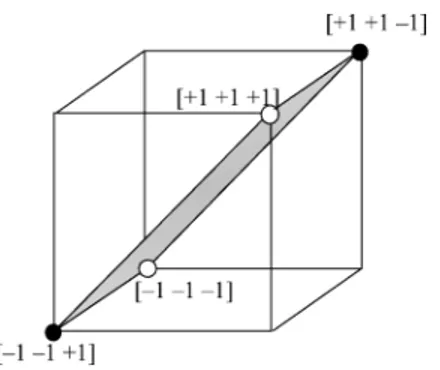
Fig. 1. Optimal separating hyperplane corresponding to the SVM solution. The SVs lie on the dashed lines.

(Fig. 1). The data points for which the constraints (2) are satisfied with the equality sign are called support vectors. Intro-ducing the Lagrange multipliers , the minimization of under constraints (2) can be recast in the following dual form [10]: Find the minimum of

(3)

subject to the linear constraints

(4) (5) Solving this QP problem, we obtain the optimum Lagrange multipliers , one for each data point. Using the Lagrange mul-tipliers we can compute the optimum weight vector as fol-lows:

(6)

Only the Lagrange multipliers corresponding to support vectors are greater than zero, so the optimum weights depend uniquely on the support vectors (SVs).

For an SV , it is

from which the optimum bias can be computed. In practice, it is better to average the values obtained by considering the set of all support vectors

(7)

where expression (6) has been used.

SVM formulation can be extended to the case of nonsepa-rable classes, introducing the slack variables ; optimal class separation can be obtained by

(8) (9a) (9b) In this case, the margin of separation is said to be soft. The constant is user-defined and controls the tradeoff be-tween the maximization of the margin and the minimization of classification errors on the training set. The dual formulation of the QP is the same as (3)–(5) with the only difference in the bound constraints, which now become:

(10) In this case, for the optimum Lagrange multipliers we have:

for support vectors for points

correctly classified with for points with

(are misclassified if ). In the soft margin case (7) still holds, but the average is taken over all such that

(generalized support vectors).

Finally, the threshold could be chosen a priori; in this case, the SVM can be trained by finding the minimum of

(11)

subject to the bound constraints

With respect to the general formulation, the equality constraint (4) disappears and it is easier to find the solution. From the optimum Lagrange multipliers, we obtain the weight vector using (6). Note that even if the classes are linearly separable, it is not guaranteed that they can be separated by the hyperplane with the threshold chosen a priori.

III. SVM DESIGN OFGBSB NEURALNETWORKS Let consider the generalized brain-state-in-a-box (GBSB) neural model described by the following difference equation2_:

(12) is the state vector;

is the number of neurons; is the weight

matrix assumed nonsymmetric; is the bias vector; is

2_{We use the same symbol for the gain}_{in (12) and the Lagrange multipliers}

introduced in Section II, complying with the literature on GBSB networks and on SVMs.

(3)

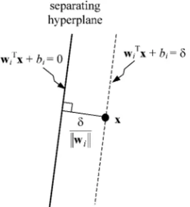
Fig. 2. Three bipolar patterns to be stored in theAM(x = [+1 + 1 0 1]; x = [01 + 1 + 1]; x = [+1 0 1 + 1]) and corresponding reduced vectors in < . The optimal separating hyperplane is shown.

a scalar; is a vector valued function, whose th component is defined as

if if

if

Let . The design of a bipolar associative

memory, based on model (12), can be formulated as follows. Synthesis Problem

Find the connection matrix and bias vector such that

1) a given set of bipolar vectors are stored as

asymptotically stable equilibrium states of system (12); 2) the basins of attraction of the desired equilibria are as large

as possible;

3) the number of not desired (spurious) stable equilibria and the number of oscillatory solutions are as small as possible. Several analysis results are available for GBSB neural net-works. In the following, we review only the most significant of them (the proofs can be found in [6] in the case ; the ex-tension to the present case is straightforward).

a) If for , only the vertices of

can be asymptotically stable equilibria of system (12). b) is an asymptotically stable equilibrium point of

system (12) if and only if

(13)

c) Assume that is an asymptotically stable equi-librium point of system (12). Then, no equiequi-librium point

exists at Hamming distance one from if , for

.

d) Let denote an asymptotically stable equilibrium

point of (12). Let differ from in the

compo-nents . If

(14)

for at least one integer then is not an

equilibrium point.

Constraints (13) represent existence and stability conditions for a given binary equilibrium point . We can design the as-sociative memory by solving (13) with respect to the weights and bias for a given set of bipolar equilibrium points . From properties and it follows that a zero-diagonal connec-tion matrix guarantees the absence of equilibria with nonbinary components, and the absence of equilibria at Hamming distance one from the desired patterns. Taking into account the stability conditions (13) and the zero-diagonal constraint, the synthesis problem for the th neuron can be recast as follows: Find and

such that

(15)

where is equal to with the th entry eliminated

and is the th row of matrix with the th entry

eliminated.

Comparing expressions (1) and (15), the design of the th neuron can be interpreted as a classification problem with

training set given by , where each

reduced vector is void of the component and belongs

to the class represented by . The synthesis

problem can be solved by a set of independent SVMs, where , computes the weight vector and bias for th neuron. The method is illustrated in Fig. 2 in the

(4)

Fig. 3. Reduced vectors in< which are not linearly separable.

three-dimensional case. The reduced vectors live in . In this simple example all three classification problems admit the same margin and all patterns are support vectors for each machine.

A similar viewpoint was adopted by Liu and Lu [11] to design a continuous-time AM by perceptrons trained by Rosenblatt’s algorithm. Using SVMs we have a maximization of the margin of separation.

Some useful relations can be found between the properties of SVMs in Section II and the design of model (12).

Property 1: Given vectors , they can be stored as asymptotically stable states of system (12) with a zero-diag-onal if and only if, for every , the corresponding reduced vectors are linearly separable in , where the classes are determined according to the th element of the desired patterns. In particular, any two vectors must differ in at least two components.

Proof: The design constraints (15) can be interpreted as finding a separating hyperplane in ; so the given set of patterns admits a solution if and only if the reduced vectors are linearly separable. Moreover, if two prototypes differ in only one component, say the th, the corresponding reduced vec-tors are identical but belong to different classes. In this case, we cannot separate them.

Property 1 is illustrated by an example. Consider the fol-lowing four patterns in

, which differ in at least two positions. Deleting the last component we obtain the coplanar vectors

shown in Fig. 3, which cannot be linearly separated. Exploiting the geometrical properties introduced by Cover [12], we can say that bipolar vectors with components can be stored with a zero-diagonal , apart from pathological cases (the re-duced vectors lie on an hyperplane in ).

In general, there are no simple criteria to predict the linear separability of the given patterns. However, using SVMs this condition can be simply checked. It is sufficient to solve the

QP with a very large value for : If for every the

given patterns are linearly separable. If at least one saturates, linear separation is not possible; in this last case, we can store a subset of the given patterns using the soft margin approach, as explained in Section IV.

Property 2: The weights of the GBSB neural network com-puted using SVMs follow a generalized Hebb’s law.

Proof: Using (6) with we have the following expression for the weights:

(16) where is the Lagrange multiplier corresponding to the th neuron and the th prototype vector. Expression (16) corre-sponds to the Hebb’s law where each product is multiplied by a real constant . Note that a subset of the Lagrange multipliers will be zero (corresponding to non-support vectors), hence not all the products will be present in (16).

Often the design of model (12) is formulated as follows [6],

[7]: Find such that

(17) where is called margin of stability. Since the weight vector can be rescaled to obtain any value for , a limitation or nor-malization of the weights is required in this formulation (e.g., ). Increasing we generally obtain less spurious stable states with larger basins of attraction. This property can be justified exploiting property of the GBSB model. Assume is a stable equilibrium point, and a random bipolar pattern with the constraint that it differs from in th compo-nent. Assuming , condition (14) can be rewritten as fol-lows:

(18)

where are random variables with values 0, and

. From th condition (13), we have

Hence, (18) becomes

(19) Let us define as the probability that (19) is true

where .

Assume are identically distributed independent

random variables, with zero mean and variance . If is large the random variable becomes normally distributed with zero mean and variance

(5)

Fig. 4. Relation between margin of stability and distance from the separating hyperplane.

Thus, we can write

(20) where denotes the error function. Increasing the ratio , the probability that points different from the desired patterns are unstable will increase; this fact favours larger basins of attraction improving the error correction ability. Expression (20) has a simple geometrical interpretation from

the classification viewpoint. The ratio

rep-resents the distance between and the th separating hyper-plane [10]; thus, is the distance between the th sep-arating hyperplane and the closest point (the margin of separa-tion) (Fig. 4). Using SVMs we minimize s.t.

(21)

Hence, we can state the following property.

Property 3: The SVM solution of the synthesis problem cor-responds to the maximum margin of separation with normalized (unitary) stability margin and minimum weight vector norm.

Remark 1: Using (21) we can easily take into account the effects of parameter quantizations. Assume the weight vector is affected by a rounding error ; in order to preserve the stability of condition (13) becomes

i.e.

Using the worst case approach and taking into account (21), we have

Assume that the weights are represented in digital form with bits, the previous condition becomes

The required number of bits to represent the weights is easily obtained

It is worth noting that this number depends only on the memory size and not on the stored patterns.

Remark 2: A second application of (21) is a preselection of the bias . Using SVMs, as explained above, some of the nega-tives of the stored patterns could be stable states (attractors) of the AM. To avoid this problem, the values can be computed as follows. The vector cannot be a stable state

if , for at least one neuron i. Assume

that is an SV for the th SVM, hence

(22)

Replacing with in (22) gives

To destabilize , it must be

hence it is sufficient that if or if

. We suggest the following expression for the bias:

(23) where is a small positive number. With this bias value will be unstable for neuron if

(24) Using (23) the sign of is selected according to the majority of or in position . In this way, we maximize the number of prototypes whose negatives are destabilized. This method does not guarantee that all the negatives are unstable, since it may happen that is an SV but condition (24) is not fulfilled. However, as evidenced by computer experiments, if we use

SVMs to store vectors, each corresponds to a

sup-port vector for most of the machines. So the probability is high that the negative is destabilized for some . Note that expression (23) is in accordance with the method suggested in [5], [7] to bias the trajectory toward one of the desired patterns.

Remark 3: No convergence results are known for model (12) with nonsymmetric matrix . However, the simulation results show that there is a strict relation between the value of in (12) and the magnitude of the weights. If we increase the magnitude of the weights, a correspondingly lower value of should be used in order to have a convergent dynamics for most initial conditions. This behavior is well known for symmetric

(6)

weight matrices; in this case convergence is guaranteed if

where represents the minimum

real eigenvalue of ; since the diagonal elements of are zero, is negative and its magnitude increases with the norm of . Using SVMs, we obtain the minimum norm weight vector satisfying the constraints, for every ; this property allows a larger for a convergent behaviour.

As concerns the practical implementation of the proposed de-sign method, we can use one of the computationally efficient packages available to solve the SVM learning problem, e.g., [13] and Libsvm [14]. In particular, Libsvm, based on Platt’s sequential minimal optimization (SMO) [15], can suc-cessfully handle classification problems with large amounts of data points – . An evaluation of the run time for the SMO algorithm can be found in [15], where some benchmark problems are solved using a 266-MHz Pentium II processor. For linear SVMs, as those considered in this paper, the computa-tion time is of the order of few seconds for problems with less than 5000 data points. Moreover, the computation time scales

between and with the number of data points.

Fi-nally, also some specialized digital hardware has been realized [16].

IV. EXPERIMENTALRESULTS

In this section, we present some design examples and sim-ulation results in order to compare the SVM design with two existing methods: The perceptron learning algorithm [11] and the designer neural network [7]. Among the many existing tech-niques for AM design, we have chosen these for three reasons: They give nonsymmetric matrices, as the present method; they are based on a constraint satisfaction formulation of the synthesis problem, as the present method; their performance is good as concerns capacity and error correction ability.

In all the experiments presented here, SVM training was car-ried out using [13] with a Matlab interface. The run time was negligible since (the number of desired patterns) is quite small. In Examples 1 and 2 the desired patterns are lin-early separable; the SVM solution was obtained using

and the values of the Lagrange multipliers were comprised be-tween 0 and 2. In Example 3 we considered different values for . As concerns the simulation of (12), in all cases the value was used, both for sake of comparison with [7] and because the networks synthesized by the perceptron learning al-gorithm often oscillate for larger values of .

Example 1: In this example, we compare the SVM solution with the design obtained using a perceptron trained by Rosen-blatt’s algorithm [11]. With this algorithm we must select a learning rate which affects the performance of the designed AM. We tried different values for ; the margins of separation

are comparable for ; for the margin can

be very small for some patterns, worsening the error correction ability. So, in the following, we present only the results obtained with . This choice presents the additional advantage of in-teger connection weights [11].

For this test, ten training sets were randomly generated; each set is composed of patterns with size

. The minimum Hamming distance between patterns is two. For each set, we found the weight matrix and bias vector

TABLE I

EXAMPLE1: BASINS OFATTRACTION

TABLE II

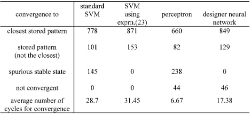
EXAMPLE1: CONVERGENCETEST FOR1024 INITIALSTATES

using the SVMs and the perceptron learning algorithm. Both methods always stored all the five vectors as asymptotically stable states. The average number of spurious stable states was 4 with the SVMs and 5.7 with the perceptron learning algorithm. Then we simulated the dynamic behavior of the GBSB network starting from initial states with Hamming distance from each of the stored prototype vectors. In Table I the results are sum-marized; they are based on ensemble averages over ten training sets. The first row represents the total number of vectors at Ham-ming distance from a stored pattern, given by . The re-maining rows represent the average number of initial states at Hamming distance from one of the stored patterns , con-verging to .

To gain a deeper insight into the behavior of the designed as-sociative memory, we simulated the dynamic evolution starting from all the 1024 bipolar initial states. Then we counted: The number of initial states converging to the closest stored pattern (in Hamming sense); the number of initial states converging to one of the stored patterns but not to the closest one; the number of initial states converging to binary spurious states and, finally, those corresponding to oscillatory solutions (convergence is not guaranteed since is nonsymmetric). These results are shown in Table II. Using SVMs, we obtain less trajectories converging to spurious stable states or not converging at all.

We examined also the capacity measure proposed in [18], based on the concept of recall accuracy (RA) for a given Ham-ming radius . represents the percentage of initial states

at Hamming distance from a stored pattern,

converging to it. For example, in Table I corresponds

to ; since in there are ten vectors with

from a given prototype, the recall accuracy is 99% with the

SVM and 84% with the perceptron. The value

(7)

at , the recall accuracy is 86% with the SVM and 58% with the perceptron. For sake of comparison we consider the re-sults in [17], based on the Ho–Kashyap method [18]: They are

% for and % for

and .

Example 2: Here, we consider a specific design example and compare four different design strategies: SVM standard, SVM with fixed threshold according to (23), perceptron, and the de-signer neural network of Chan and Zak. Let us consider the five patterns with shown at the bottom of the page, to be stored in the associative memory (it is the same example con-sidered in [6] and [7]).

The weight matrix and bias vector are given in (25), as shown at the bottom of the page. All the prototype vectors are stored, along with five spurious states. The same problem

was solved computing the bias by (23) with . In

this case, all the vectors were stored, with no spurious states. The weight matrix and bias vector are given in (26), as shown at the bottom of the page. Then we solved the design problem using the perceptron learning algorithm, with

: all the prototypes were stored, with seven spurious stable states. The solution is shown in (27)

(27a)

(27b) The designer neural network stores the desired vectors without spurious states (W and b in [7, p. 366]).

(25a)

(25b)

(26a)

(8)

TABLE III

EXAMPLE2: BASINS OFATTRACTION—STANDARDSVM

TABLE IV

EXAMPLE2: BASINS OFATTRACTION—SVM WITHBIASGIVEN BY(23)

TABLE V

EXAMPLE2: BASINS OFATTRACTION—PERCEPTRON

TABLE VI

EXAMPLE2: BASINS OFATTRACTION—DESIGNERNEURALNETWORK

Then, we simulated the dynamic behaviour of the GBSB net-work starting from the initial states with Hamming distance 1 , from each of the stored prototype vectors. The re-sults are shown in Tables III–VI, where the entry at intersec-tion of row and column represents the number of initial states at Hamming distance from converging to . Fi-nally, we simulated the dynamic evolution starting from all the 1024 bipolar initial states. These results are shown in Table VII. From the simulation results, we see that standard SVMs give larger basins of attraction and less spurious states with respect to the perceptron learning algorithm. Using SVMs with the bias computed by (23) we obtain results comparable to those of Chan and Zak [7]. As concerns the convergence speed, the data in Table VII confirm the comments in Remark 3 of Section III.

The networks synthesized using SVMs have a minimum norm weight vector; as a consequence the dynamic evolution is slower but the chance of oscillation is rare.

An important advantage of the proposed approach is that stan-dard software routines for SVMs can be used without the need for special-purpose analog circuits, as those proposed in [7], [8]. Finally, there are no design parameters to be tuned. This is a major difference with respect to both the perceptron, where the learning rate can influence the results, and to the designer neural network, where some circuit parameters must be selected (input voltage source, slope of the piecewise-linear amplifiers, stability margin).

Example 3: In this example, we consider vectors and try to store them in the AM. Even when a solution to the problem does not exist, using SVMs we can store a subset of the given prototype vectors, trading off the number of successfully stored patterns and their recall accuracy. This is possible by using the soft margin constraints (10). Varying the penalty parameter we can find several solutions with different stored patterns and margin of separation. To verify this property, we consider the following 12 vectors of size

(28)

The minimum Hamming distance between patterns is two. We computed the weight matrix and bias vector using several values of (the same is used for each SVM). In Table VIII, some design examples are summarized. They correspond to the largest number of stored patterns; for the values of not shown in Table VIII we obtained less than seven stored vectors out of twelve. Table VIII shows: The number of successfully stored patterns, the RA for , the number of spurious stable states. The value denotes the positive infinity in Matlab; it corresponds to unbounded values for the Lagrange multipliers, as in (5).

Note that the twelve vectors can simultaneously be stored as stable states, i.e., they can be linearly separated by each neuron. This is obtained by using . However this solution corre-sponds to the minimum recall accuracy. Note that RA decreases with . This behaviour can easily be explained observing the QP (8) and (9). Larger values of correspond to SVM solu-tions with reduced margin of separation, i.e., smaller attraction basins.

(9)

TABLE VII

EXAMPLE2: CONVERGENCETEST FOR1024 INITIALSTATES

TABLE VIII EXAMPLE3: VECTORS(28)

TABLE IX EXAMPLE3: VECTORS(29)

As a further example, we consider the following 12 vectors

of size :

(29) The minimum Hamming distance is two. In this case the twelve vectors cannot be simultaneously stored in the AM. At most ten vectors can be stored, with . The results for some values of are summarized in Table IX.

V. COMMENTS ANDCONCLUSIONS

We showed how the design of a recurrent associative memory can be recast as a classification problem and efficiently solved using a pool of SVMs. We pointed out some properties of the

associative memories designed in this way, as the generalized Hebb’s law. The proposed approach presents some interesting features. First of all, if the design problem admits a solution, the proposed approach gives the “optimal” one, i.e., that with the largest margin of separation. As a consequence of the maxi-mization of the margin, the recall accuracy of the stored patterns compares well with existing techniques for associative memory design. Moreover, the SVM solution allows a simple method to control the effect of parameter quantization and to avoid, with high probability, the storage of the negatives of the desired pat-terns. Further, the minimization of weight vector norm, implicit in the SVM solution, helps to obtain a convergent dynamic be-haviour in the recall phase, even if the connection matrix is non-symmetric. Another practical advantage of the proposed method is the absence of design parameters, at least in the usual case when a given set of (linearly separable) patterns must be stored. However, the SVM approach gives a further benefit: It allows to tradeoff capacity and recall accuracy in a simple way, by varying the design parameter .

REFERENCES

[1] J. J. Hopfield, “Neural networks and physical systems with emergent collective computational abilities,” in Proc. Natl. Acad. Sci., 1982, vol. 79, pp. 2554–2558.

[2] J. M. Zurada, Introduction to Artificial Neural Systems. St. Paul, MN: West, 1992.

[3] A. N. Michel and J. A. Farrell, “Associative memories via artificial neural networks,” IEEE Control Syst. Mag., vol. 10, no. 3, pp. 6–17, Apr. 1990.

[4] S. Hui and S. H. Zak, “Dynamical analysis of the brain-state-in-a-box (BSB) neural models,” IEEE Trans. Neural Netw., vol. 3, no. 1, pp. 86–100, Jan. 1992.

[5] W. E. Lillo, D. C. Miller, S. Hui, and S. H. Zak, “Synthesis of brain-state-in-a-box (BSB) based associative memories,” IEEE Trans. Neural Netw., vol. 5, no. 5, pp. 730–737, Sep. 1994.

[6] R. Perfetti, “A synthesis procedure for brain-state-in-a-box neural net-works,” IEEE Trans. Neural Netw., vol. 6, no. 5, pp. 1071–1080, Sep. 1995.

[7] H. Y. Chan and S. H. Zak, “On neural networks that design neural associative memories,” IEEE Trans. Neural Netw., vol. 8, no. 2, pp. 360–372, Mar. 1997.

[8] R. Perfetti, “A neural network to design neural networks,” IEEE Trans. Circuits Syst., vol. 38, no. 9, pp. 1099–1103, Sep. 1991.

[9] C. J. C. Burges, “A tutorial on support vector machines for pattern recognition,” in Data Mining and Knowledge Discovery. Norwell, MA: Kluwer, 1998, vol. 2, pp. 121–167.

[10] S. Haykin, Neural Networks: A Comprehensive Foundation, 2nd ed. Upper Saddle River, NJ: Prentice-Hall, 1999.

[11] D. Liu and Z. Lu, “A new synthesis approach for feedback neural net-works based on the perceptron training algorithm,” IEEE Trans. Neural Netw., vol. 8, no. 6, pp. 1468–1482, Nov. 1997.

(10)

[12] T. M. Cover, “Geometrical and statistical properties of systems of linear inequalities with applications in pattern recognition,” IEEE Trans. Electron. Comput., vol. EC-14, no. 3, pp. 326–334, Jun. 1965. [13] T. Joachims, “Making large scale SVM learning practical,” in Advances

in Kernel Methods-Support Vector Learning, B. Scholkopf, C. J. C. Burges, and A. J. Smola, Eds. Cambridge, MA: MIT Press, 1999, pp. 169–184 [Online]. Available: http://svmlight.joachims.org/ [14] C.-C. Chang and C.-J. Lin, LIBSVM—A library for support vector

ma-chines [Online]. Available: http://www.csie.ntu.edu.tw/~cjlin/libsvm/ [15] J. C. Platt, “Fast training of support vector machines using

sequen-tial minimal optimization,” in Advances in Kernel Methods—Support Vector Learning, B. Scholkopf, C. Burges, and A. J. Smola, Eds. Cambridge, MA: MIT Press, 1999, pp. 185–208.

[16] R. Genov and G. Cauwenberghs, “Kerneltron: Support vector machine in silicon,” IEEE Trans. Neural Netw., vol. 14, no. 5, pp. 1426–1434, Sep. 2003.

[17] M. H. Hassoun and A. M. Youssef, “Associative neural memory capacity and dynamics,” in Proc. Int. J. Conf. Neural Networks, San Diego, CA, 1990, vol. 1, pp. 736–769.

[18] M. H. Hassoun and A. M. Youssef, “High performance recording al-gorithm for Hopfield model associative memories,” Opt. Eng., vol. 28, no. 1, pp. 46–54, 1989.

Daniele Casali was born in Italy in 1974. He

re-ceived the M.S. degree in electronic engineering and the Ph.D. degree in sensory and learning systems, both from the University of Rome “Tor Vergata,” Italy, in 2000 and 2004, respectively.

Currently, he is a Postdoctoral Research Assistant at the University of Rome, and has teaching assign-ments at the Faculties of Engineering and Science at the same university. His research interests include neural networks, image, and audio signal processing.

Giovanni Costantini was born in Italy in 1965. He

received the electronic engineering Laurea degree from the University of Rome “La Sapienza,” Italy, and the Ph.D. degree in telecommunication and microelectronics from the University of Rome “Tor Vergata,” Italy, in 1991 and 1999, respectively. He also graduated in piano and electronic music from the Music Conservatory, Italy.

Currently, he is an Assistant Professor at the Uni-versity of Rome, “Tor Vergata.” His primary research interests are in the fields of neural networks, pattern recognition, algorithms, and systems for audio and musical signal processing.

Renzo Perfetti was born in Italy in 1958. He

re-ceived the Laurea degree (with honors) in electronic engineering from the University of Ancona, Italy, and the Ph.D. degree in information and commu-nication engineering from the University of Rome, “La Sapienza,” Italy, in 1982 and 1992, respectively. From 1983 to 1987, he was with the radar division of Selenia, Rome, Italy, where he worked on radar systems design and simulation. From 1987 to 1992, he was with the radiocommunication division of Fon-dazione Bordoni, Rome, Italy. In 1992, he joined the Department of Electronic and Information Engineering of the University of Pe-rugia, Italy, where he is currently a Full Professor of electrical engineering. His current research interests include artificial neural networks, pattern recognition, machine learning, and digital signal processing.

Elisa Ricci received the M.S. degree in electronic

engineering from the University of Perugia, Italy, in 2003. She is currently working toward the Ph.D. de-gree in the Department of Electronic and Information Engineering, University of Perugia.

Her research interests include machine learning, neural networks, and image processing.