Fault detection, diagnosis and active fault tolerant control for a satellite attitude control system

A

M

S

-

U

B

ARCES

-

A

R

C

E

S

I

C

T

E.

D

C

D

T

’I

C

XXVII

Settore Concorsuale di afferenza: 09/G1 Settore Scientifico disciplinare: ING-INF/04

F

D

,

D

A

F

T

C

S

A

C

S

Tesi di dottorato presentata da

Pietro Baldi

Coordinatore di dottorato Relatore

Prof. Claudio Fiegna Prof. Paolo Castaldi

i

Abstract

Modern control systems are becoming more and more complex and control algorithms more and more sophisticated. Consequently, Fault Detection and Diagnosis (FDD) and Fault Tolerant Control (FTC) have gained central importance over the past decades, due to the increasing requirements of availability, cost efficiency, reliability and operating safety.

This thesis deals with the FDD and FTC problems in a spacecraft Attitude Determination and Control System (ADCS). Firstly, the detailed nonlinear models of the spacecraft attitude dynamics and kinematics are described, along with the dynamic models of the actuators and main external disturbance sources. The considered ADCS is composed of an array of four redundant reaction wheels. A set of sensors provides satellite angular velocity, attitude and flywheel spin rate information. Then, general overviews of the Fault Detection and Isolation (FDI), Fault Estimation (FE) and Fault Tolerant Control (FTC) problems are presented, and the design and implementation of a novel diagnosis system is described. The system consists of a FDI module composed of properly organized model-based residual filters, exploiting the available input and output information for the detection and localization of an occurred fault. A proper fault mapping procedure and the nonlinear geometric approach are exploited to design residual filters explicitly decoupled from the external aerodynamic disturbance and sensitive to specific sets of faults. The subsequent use of suitable adaptive FE algorithms, based on the exploitation of radial basis function neural networks, allows to obtain accurate fault estimations.

Finally, this estimation is actively exploited in a FTC scheme to achieve a suitable fault accommodation and guarantee the desired control performances. A standard sliding mode controller is implemented for attitude stabilization and control. Several simulation results are given to highlight the performances of the overall designed system in case of different types of faults affecting the ADCS actuators and sensors.

iii

Acknowledgments

Firstly, at the end of these three years, I wish to express my utmost gratitude and appreciation to my Ph.D. tutor, Prof. Paolo Castaldi, for his academic support and guidance, valuable suggestions and insightful criticism, and for his friendship, patience, constant spur and encouragement during these years.

Secondly, I wish to thanks Prof. Silvio Simani, from the Department of Engineering of the University of Ferrara, and Ing. Nicola Mimmo, from the Department of Electrical, Electronic and Information Engineering of the University of Bologna, for their friendship, helpful comments and contributions to the realization of this thesis.

Moreover, I would like to thank also all the other my colleagues at the laboratories of the Aerospace Engineering faculty in Forlì for their friendship and support during this experience, in particular Prof. Matteo Zanzi, Ing. Antonio Ghetti and Ing. Alessandro Mirri.

Part of this work has been developed while I was visiting the Department of Electrical Engineering of the Technical University of Denmark in Kogens-Lingby (DK). I want to express my sincere thanks to Prof. Mogens Blanke, who was my supervisor during my stay and gave me valuable suggestions. I wish also to thank, beside the staff of the Department, all the people of the Automation and Control Group who made my stay there pleasant and profitable.

Finally, a very special thanks to my parents and relatives for their unconditioned love and continuous support and encouragement in persevering in my research activity, and without whom this work would have been much harder to carry out.

v

Contents

1 Introduction ... 1

1.1 Fault Diagnosis and Fault Tolerant Control ... 1

1.2 Thesis Contributions ... 3

1.3 Thesis Outline ... 5

2 Spacecraft Attitude Dynamics ... 7

2.1 Reference Frames ... 7

2.1.1 Inertial Reference Frame F ... 7_i 2.1.2 Orbital Reference Frame F ... 8_o 2.1.3 Body Reference Frame F ... 8_b 2.1.4 Principal Axis of Inertia ... 9

2.2 Attitude Representations ... 9 2.2.1 Rotation Matrix ... 10 2.2.2 Euler Angles ... 12 2.2.3 Unit Quaternion... 13 2.3 Angular Velocity ... 16 2.4 Equations of Motion... 17

2.4.1 Spacecraft Inertia Matrix ... 17

2.4.2 Dynamic Equations of Motion ... 18

2.4.3 Kinematic Equations of Motion ... 20

2.5 Environmental Disturbance Torques ... 21

2.5.1 Gravity-Gradient Torque... 22

2.5.2 Aerodynamic Torque ... 25

2.5.3 Ignored Torques ... 27

2.6 Attitude Determination and Control System ... 27

2.6.1 Reaction Wheel ... 28

2.6.2 Star Tracker ... 31

2.6.3 Rate Gyro ... 34

3 Model-based Fault Detection and Isolation ... 37

3.1 General Overview ... 37

3.2 Residual Generators for Model-based FDI ... 41

3.3 Fault Isolability and Structured Residual Set ... 44

3.4 Fault Classification ... 45

3.5 Modelling of Faults for the Design of the FDI System... 50

3.5.1 Modelling of Actuator Faults ... 51

3.5.2 Modelling of Sensor Faults ... 51

3.6 Nonlinear Geometric Approach ... 53

3.7 Residual Generator Design ... 59

4 FDI Implementation in the Satellite ADCS ... 63

4.1 Mathematical Fault Inputs Associated to Physical Faults ... 63

4.2 Design of Aerodynamic Decoupled Residual Generators for FDI ... 74

4.3 Supervisor Decision Logic for Fault Isolation ... 84

4.4 Simulation Results ... 87

4.4.1 Considered fault scenarios: ... 87

4.4.2 Detection and Isolation of Faults in the Satellite ACS ... 90

4.4.3 Detection and Isolation of Faults in the Satellite ADS ... 98

5 Fault Detection and Diagnosis ... 109

5.1 General Overview ... 109

5.2 Fault Diagnosis Based on NLGA and Neural Networks ... 111

5.2.1 Radial Basis Function Neural Networks ... 111

vi

6 FDD Implementation in the Satellite ADCS ... 117

6.1 Design of Adaptive RBF-NN Filters for Fault Estimation in the Satellite ACS ... 117

6.2 Design of Adaptive RBF-NN Filters for Fault Estimation in the Satellite ADS ... 120

6.3 Simulation Results ... 123

6.3.1 Estimation of Faults in the Satellite ACS ... 123

6.3.2 Estimation of Faults in the Satellite ADS ... 136

7 Fault Tolerant Control ... 143

7.1 General Overview ... 143

7.2 Control Reconfiguration and Fault Accommodation ... 147

7.3 Reconfiguration Mechanism ... 149

8 FTC Implementation in the Satellite ADCS ... 151

8.1 Sliding Mode Control... 151

8.1.1 Sliding Surface Design... 153

8.1.2 Control Law Design ... 153

8.1.3 Chattering Avoidance and Control Input Saturation... 154

8.1.4 Controller Stability in Nominal Condition... 155

8.2 Simulation Results ... 156

8.2.1 Controller Reconfiguration after Actuator Failure... 156

8.2.2 Fault Accommodation after Actuator and Sensor Faults in the Satellite ACS ... 158

8.2.3 Fault Accommodation after Sensor Faults in the Satellite ADS ... 170

9 Conclusion... 179

10 Publications... 181

vii

List of Figures

Figure 2.1 - Earth-centred inertial reference frame. ... 8

Figure 2.2 - Local Vertical Local Horizontal (LVLH) orbital reference frame. ... 8

Figure 2.3 - Earth centred inertial, orbital and body reference frames. ... 9

Figure 2.4 - Comparison of Environmental Torques (adapted from Hughes 1986). ... 22

Figure 2.5 – Tetrahedral configuration of the satellite reaction wheels... 30

Figure 3.1 - Topological illustration of fault diagnosis functional relationships (Sun 2013). ... 38

Figure 3.2 - Comparison between FDI hardware redundancy and open-loop analytical (software) redundancy concepts (Sun 2013). ... 39

Figure 3.3 - Classification of explicit and quantitative model-based FDI/FDD methods (Shi 2013). ... 40

Figure 3.4 - Schematic description of model-based approach to FDI (Sun 2013). ... 41

Figure 3.5 - Redundant signal structure in residual generation. ... 42

Figure 3.6 - Fault diagnosis and control loop. ... 43

Figure 3.7 - Structured dedicated residual set for three distinct faults. ... 44

Figure 3.8 - Structured generalized residual set for three distinct faults. ... 45

Figure 3.9 - Actuator fault, sensor fault and component faults (Sun 2013). ... 46

Figure 3.10 - Abrupt fault, incipient fault and intermittent fault (Sun 2013). ... 47

Figure 3.11 - Additive fault and multiplicative fault (Sun 2013). ... 48

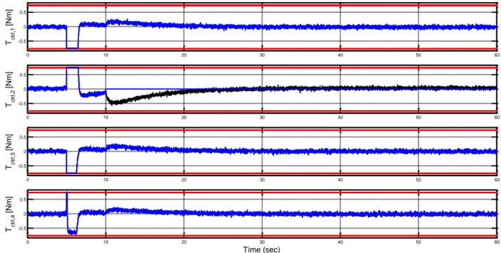
Figure 4.1 - Fault scenario n.1: local residuals of RB1 sensitive to fault inputs associated to physical actuator and flywheel spin rate sensor faults in case of step fault on the control input T_ctrl,2. ... 90

Figure 4.2 - Fault scenario n.1: global residuals of RB2 not sensitive to any fault input associated to physical actuator faults in case of step fault on the control input T_ctrl,2. ... 91

Figure 4.3 - Fault scenario n.2: local residuals of RB1 sensitive to fault inputs associated to physical actuator and flywheel spin rate sensor faults in case of sinusoidal fault on the control input T_ctrl,2. . 91

Figure 4.4 - Fault scenario n.2: global residuals of RB2 not sensitive to any fault input associated to physical actuator faults in case of sinusoidal fault on the control input T_ctrl,2. ... 92

Figure 4.5 - Fault scenario n.3: local residuals of RB1 sensitive to fault inputs associated to physical actuator and flywheel spin rate sensor faults in case of rectangular pulse fault on the control input ,2 ctrl T . ... 92

Figure 4.6 - Fault scenario n.3: global residuals of RB2 not sensitive to any fault input associated to physical actuator faults in case of rectangular pulse fault on the control input T_ctrl,2. ... 93

Figure 4.7 - Fault scenario n.4: local residuals of RB1 sensitive to fault inputs associated to physical actuator and flywheel spin rate sensor faults in case of ramp fault on the control input T_ctrl,2. ... 93

Figure 4.8 - Fault scenario n.4: global residuals of RB2 not sensitive to any fault input associated to physical actuator faults in case of ramp fault on the control input T_ctrl,2. ... 94

Figure 4.9 - Fault scenario n.5: local residuals of RB1 sensitive to fault inputs associated to physical actuator faults and corresponding flywheel spin rate sensor faults in case of failure of the second actuator. ... 94

Figure 4.10 - Fault scenario n.5: global residuals of RB2 not sensitive to any fault input associated to physical actuator faults in case of failure of the second actuator. ... 95

Figure 4.11 - Fault scenario n.6: local residuals of RB1 sensitive to fault inputs associated to physical actuator faults and corresponding flywheel spin rate sensor faults in case of step fault on the sensor output _,3 measured w  . ... 96

Figure 4.12 - Fault scenario n.6: global residuals of RB2 not sensitive to any fault input associated to physical actuator faults in case of step fault on the sensor output _,3 measured w  . ... 96

viii

Figure 4.13 - Fault scenario n.7: local residuals of RB1 sensitive to fault inputs associated to

physical actuator faults and corresponding flywheel spin rate sensor faults in case of sinusoidal fault on the sensor output _,3

measured w

 . ... 97 Figure 4.14 - Fault scenario n.7: global residuals of RB2 not sensitive to any fault input associated to physical actuator faults in case of sinusoidal fault on the sensor output _,3

measured w

 . ... 97 Figure 4.15 - Fault scenario n.8: local residuals of RB1 sensitive to fault inputs associated to

physical actuator faults and corresponding flywheel spin rate sensor faults in case of failure of the sensor measuring _w,3. ... 98 Figure 4.16 - Fault scenario n.8: global residuals of RB2 not sensitive to any fault input associated to physical actuator torque faults. In this case, all the global residuals exceed the selected thresholds in case of failure of the sensor measuring _w,3. ... 98 Figure 4.17 - Fault scenario n.9: residuals of RB3, sensitive to fault inputs associated to the physical faults affecting the sensors measuring _{x i,} and _{y i,} , in case of step fault on the sensor output

,measured x i

 . ... 99 Figure 4.18 - Fault scenario n.9: residuals of RB3, sensitive to fault inputs associated to the physical faults affecting the sensors measuring _{x i,} and _{z i,} , in case of step fault on the sensor output

,measured x i

 . ... 100 Figure 4.19 - Fault scenario n.9: residuals of RB3, sensitive to fault inputs associated to the physical faults affecting the sensors measuring _{y i,} and _{z i,} , in case of step fault on the sensor output

,measured x i

 . ... 100 Figure 4.20 - Fault scenario n.9: residuals of RB4, sensitive to fault inputs associated to the physical faults affecting the sensors measuring _{x i,} and _{y i,} , in case of step fault on the sensor output

,measured x i

 . ... 101 Figure 4.21 - Fault scenario n.9: residuals of RB4, sensitive to fault inputs associated to the physical faults affecting the sensors measuring _{x i,} and _{z i,} , in case of step fault on the sensor output

,measured x i

 . ... 101 Figure 4.22 - Fault scenario n.9: residuals of RB4, sensitive to fault inputs associated to the physical faults affecting the sensors measuring _{y i,} and _{z i,} , in case of step fault on the sensor output

,measured x i

 . ... 102 Figure 4.23 - Fault scenario n.10: residuals of RB4, sensitive to fault inputs associated to the

physical faults affecting the sensors measuring _{x i,} and _{y i,} , in case of lock-in-place fault on the sensor output _,

measured x i

 . ... 102 Figure 4.24 - Fault scenario n.10: residuals of RB3, sensitive to fault inputs associated to the

physical faults affecting the sensors measuring _{x i,} and _{z i,} , in case of lock-in-place fault on the sensor output _,

measured x i

 . ... 103 Figure 4.25 - Fault scenario n.10: residuals of RB3, sensitive to fault inputs associated to the

physical faults affecting the sensors measuring _{y i,} and _{z i,} , in case of lock-in-place fault on the sensor output _,

measured x i

 . ... 103 Figure 4.26 - Fault scenario n.11: residuals of RB3, sensitive to fault inputs associated to the

physical faults affecting the sensors measuring _{x i,} and _{y i,} , in case of loss-of-effectiveness fault on the sensor output _,

measured x i

ix Figure 4.27 - Fault scenario n.11: residuals of RB3, sensitive to fault inputs associated to the

physical faults affecting the sensors measuring _{x i,} and _{z i,} , in case of loss-of-effectiveness fault on the sensor output _,

measured x i

 . ... 104

Figure 4.28 - Fault scenario n.11: residuals of RB3, sensitive to fault inputs associated to the physical faults affecting the sensors measuring _{y i,} and _{z i,} , in case of loss-of-effectiveness fault on the sensor output _, measured x i  . ... 105

Figure 4.29 - Fault scenario n.12: residuals of RB3, sensitive to fault inputs associated to the physical faults on the sensor measuring _{x i,}, _{y i,} and q_star1, in case of fault on the first measured attitude quaternion vector. ... 106

Figure 4.30 - Fault scenario n.12: residuals of RB3, sensitive to fault inputs associated to the physical faults on the sensor measuring _{x i,}, _{z i,} and q_star1, in case of fault on the first measured attitude quaternion vector. ... 106

Figure 4.31 - Fault scenario n.12: residuals of RB3, sensitive to fault inputs associated to the physical faults on the sensor measuring _{y i,} , _{z i,} and q_star1, in case of fault on the first measured attitude quaternion vector. ... 107

Figure 4.32 - Fault scenario n.12: residuals of RB4, sensitive to fault inputs associated to the physical faults on the sensor measuring _{x i,}, _{y i,} and q_star2, in case of fault on the first measured attitude quaternion vector. ... 107

Figure 4.33 - Fault scenario n.12: residuals of RB4, sensitive to fault inputs associated to the physical faults on the sensor measuring _{x i,}, _{z i,} and q_star2, in case of fault on the first measured attitude quaternion vector. ... 108

Figure 4.34 - Fault scenario n.12: residuals of RB4, sensitive to fault inputs associated to the physical faults on the sensor measuring _{y i,} , _{z i,} and q_star2, in case of fault on the first measured attitude quaternion vector. ... 108

Figure 5.1 - Schematic description of model-based FDD method (Sun 2013). ... 110

Figure 5.2 - Observer-based FDI/FDD schemes (Sun 2013). ... 111

Figure 5.3 - Schematic representation of RBF neural network... 112

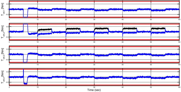
Figure 6.1 - Fault scenario n.1: commanded (black) and actuated (blue) control inputs T and _c T_ctrl in case of step fault on the control input T_ctrl,2. ... 124

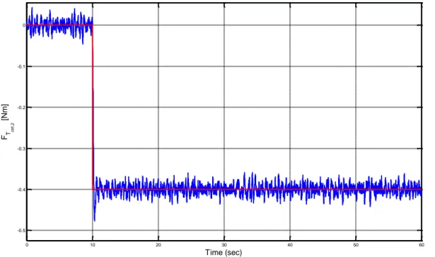
Figure 6.2 - Fault scenario n.1: true (red) and estimated (blue) step fault on the control input T_ctrl,2. ... 124

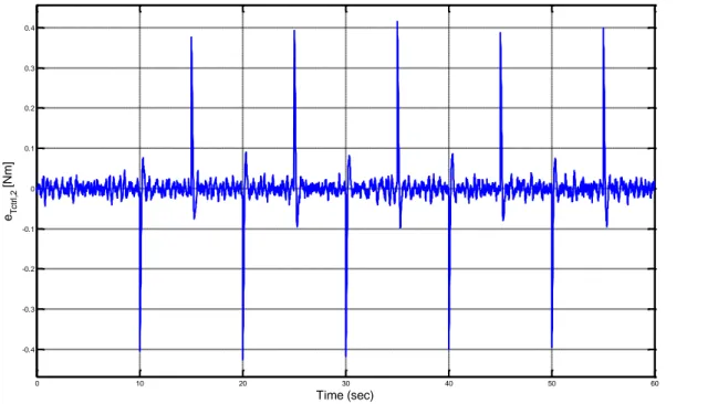
Figure 6.3 - Fault scenario n.1: estimation error for the step fault on the control input T_ctrl,2. ... 125

Figure 6.4 - Fault scenario n.2: commanded (black) and actuated (blue) control inputs T and _c T_ctrl in case of sinusoidal fault on the control input T_ctrl,2. ... 126

Figure 6.5 - Fault scenario n.2: true (red) and estimated (blue) sinusoidal fault on the control input ,2 ctrl T . ... 126

Figure 6.6 - Fault scenario n.2: estimation error for the sinusoidal fault on the control input T_ctrl,2. ... 127

Figure 6.7 - Fault scenario n.3: commanded (black) and actuated (blue) control inputs T and _c T_ctrl in case of rectangular pulse fault on the control input T_ctrl,2. ... 127

Figure 6.8 - Fault scenario n.3: true (red) and estimated (blue) rectangular pulse fault on the control input T_ctrl,2. ... 128

Figure 6.9 - Fault scenario n.3: estimation error for the rectangular pulse fault on the control input ,2 ctrl T . ... 128

x

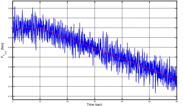
Figure 6.10 - Fault scenario n.4: commanded (black) and actuated (blue) control inputs T and _c T_ctrl in case of ramp fault on the control input T_ctrl,2. ... 129 Figure 6.11 - Fault scenario n.4: true (red) and estimated (blue) ramp fault on the control input

,2

ctrl

T . ... 129 Figure 6.12 - Fault scenario n.4: estimation error for the ramp fault on the control input T_ctrl,2. .... 130 Figure 6.13 - Fault scenario n.5: commanded (black) and actuated (blue) control inputs T and _c T_ctrl in case of failure of the actuator providing the control input T_ctrl,2. ... 130 Figure 6.14 - Fault scenario n.5: true (red) and estimated (blue) fault corresponding to the failure of the actuator providing the control input T_ctrl,2. ... 131 Figure 6.15 - Fault scenario n.5: estimation error of the fault corresponding to the failure of the actuator providing the control input T_ctrl,2. ... 131 Figure 6.16 - Fault scenario n.6: true (black) and measured (blue) flywheel spin rates _w in case of step fault on the sensor output _,3

measured w

 ... 132 Figure 6.17 - Fault scenario n.6: true (red) and estimated (blue) step fault on the sensor output

,3measured w

 . ... 132 Figure 6.18 - Fault scenario n.6: estimation error for the step fault on the sensor output _,3

measured w

 .133

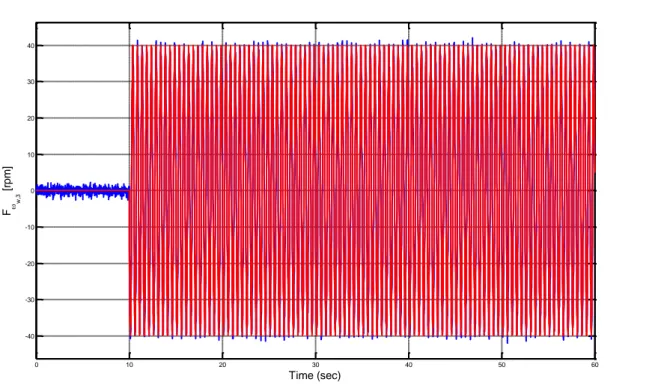
Figure 6.19 - Fault scenario n.7: true (black) and measured (blue) flywheel spin rates _w in case of sinusoidal fault on the sensor output _,3

measured w

 . ... 133 Figure 6.20 - Fault scenario n.7: true (red) and estimated (blue) sinusoidal fault on the sensor output

,3measured w

 . ... 134 Figure 6.21 - Fault scenario n.7: estimation error for the sinusoidal fault on the sensor output

,3measured w

 . ... 134 Figure 6.22 - Fault scenario n.8: true (black) and measured (blue) flywheel spin rates _w in case of failure of the sensor measuring _w,3. ... 135 Figure 6.23 - Fault scenario n.8: true (red) and estimated (blue) fault corresponding to the failure of the sensor measuring _w,3. ... 135 Figure 6.24 - Fault scenario n.8: estimation error of the fault corresponding to the failure of the sensor measuring _,3

measured w

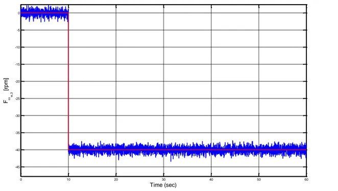
 . ... 136 Figure 6.25 - Fault scenario n.9: true (black) and measured (blue) satellite angular velocity  in case of step fault on the sensor output _,

measured x i

 . ... 137 Figure 6.26 - Fault scenario n.9: true (red) and estimated (blue) step fault on the sensor output

,measured x i

 . ... 137 Figure 6.27 - Fault scenario n.9: estimation error for the step fault on the sensor output _,

measured x i

 . 138

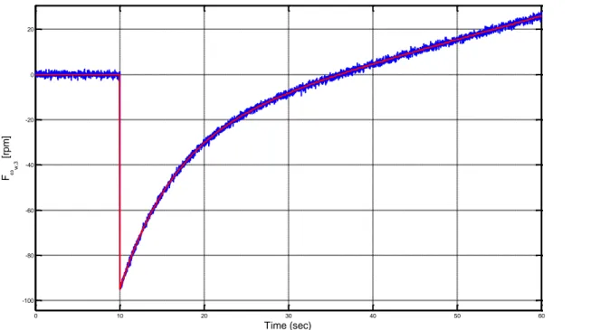
Figure 6.28 - Fault scenario n.10: true (black) and measured (blue) satellite angular velocity  in case of lock-in-place fault on the sensor output _,

measured x i

 . ... 138 Figure 6.29 - Fault scenario n.10: true (red) and estimated (blue) lock-in-place fault on the sensor output _,

measured x i

 . ... 139 Figure 6.30 - Fault scenario n.10: estimation error for the lock-in-place fault on the sensor output

,measured x i

 . ... 139 Figure 6.31 - Fault scenario n.11: true (black) and measured (blue) satellite angular velocity  in case of loss-of-effectiveness fault on the sensor output _,

measured x i

 . ... 140 Figure 6.32 - Fault scenario n.11: true (red) and estimated (blue) loss-of-effectiveness fault on the sensor output _,

measured x i

xi Figure 6.33 - Fault scenario n.11: estimation error for the loss-of-effectiveness fault on the sensor output _,

measured x i

 . ... 141

Figure 6.34 - Fault scenario n.12: true (black) and measured (blue) attitude quaternion vector q_star1 in case of fault on the first attitude sensor output. ... 141

Figure 6.35 - Fault scenario n.12: true (red) and estimated (blue) additive fault vector associated to the physical fault on the sensor measuring the attitude quaternion vector q_star1. ... 142

Figure 6.36 - Fault scenario n.12: estimation error of the additive fault vector associated to the physical fault on the sensor measuring the attitude quaternion vector q_star1. ... 142

Figure 7.1 - Classification of the main regions of operation, based on FTC requirements (Blanke et al. 2006). ... 144

Figure 7.2 - Architecture of an active fault tolerant control (Blanke et al. 2006). ... 146

Figure 7.3 - Schematic structure of AFTC systems (Sun 2013). ... 146

Figure 7.4 - Classification of control reconfiguration methods (Lunze and Richter 2008). ... 147

Figure 7.5 - Control reconfiguration (Blanke et al. 2006). ... 148

Figure 7.6 - Fault accommodation (Blanke et al. 2006). ... 149

Figure 8.1 - Error phase-plane for different gain values (Ibrahim et al. 2012). ... 154

Figure 8.2 - Fault scenario n.5: commanded (black) and actuated (blue) control inputs T and _c T_ctrl in case of failure of the actuator providing the control input T_ctrl,2. ... 157

Figure 8.3 - Fault scenario n.5: commanded (black) and actuated (blue) control inputs T and _c T_ctrl in case of failure of the actuator providing the control input T_ctrl,2. The second line is excluded from the control allocation. ... 158

Figure 8.4 - Fault scenario n.5: local residuals of RB1 in case of failure of the actuator providing the control input T_ctrl,2 and subsequent control reallocation. ... 158

Figure 8.5 - Fault scenario n.1: commanded (black) and actuated (blue) control inputs T and _c T_ctrl in case of step fault on the control input T_ctrl,2 and without fault accommodation. ... 159

Figure 8.6 - Fault scenario n.1: faulty (black) and accommodated (blue) actuated control inputs T_ctrl in case of step fault on the control input T_ctrl,2 and with fault accommodation. ... 159

Figure 8.7 – Fault scenario n.1: Euler angles evolution in case of step fault on the control input ,2 ctrl T and without fault accommodation. ... 160

Figure 8.8 – Fault scenario n.1: Euler angles evolution in case of step fault on the control input ,2 ctrl T and with fault accommodation. ... 160

Figure 8.9 - Fault scenario n.1: local residuals of RB1 in case of step fault on the attitude control input T_ctrl,2 and subsequent fault accommodation. ... 161

Figure 8.10 - Fault scenario n.2: commanded (black) and actuated (blue) control inputs T and _c T_ctrl in case of sinusoidal fault on the control input T_ctrl,2 and without fault accommodation. ... 161

Figure 8.11 - Fault scenario n.2: faulty (black) and accommodated (blue) actuated control inputs ctrl T in case of sinusoidal fault on the control input T_ctrl,2 and with fault accommodation. ... 162

Figure 8.12 - Fault scenario n.2: local residuals of RB1 in case of sinusoidal fault on the attitude control input T_ctrl,2 and subsequent fault accommodation. ... 162

Figure 8.13 - Fault scenario n.3: commanded (black) and actuated (blue) control inputs T and _c T_ctrl in case of rectangular pulse fault on the control input T_ctrl,2 and without fault accommodation. .... 163

Figure 8.14 - Fault scenario n.3: faulty (black) and accommodated (blue) actuated control inputs ctrl T in case of rectangular pulse fault on the control input T_ctrl,2 and with fault accommodation. . 163

Figure 8.15 - Fault scenario n.3: local residuals of RB1 in case of rectangular pulse fault on the attitude control input T_ctrl,2 and subsequent fault accommodation. ... 164

xii

Figure 8.16 - Fault scenario n.4: commanded (black) and actuated (blue) control inputs T and _c T_ctrl in case of ramp fault on the control input T_ctrl,2 and without fault accommodation. ... 164 Figure 8.17 - Fault scenario n.4: faulty (black) and accommodated (blue) actuated control inputs

ctrl

T in case of ramp fault on the control input T_ctrl,2 and with fault accommodation. ... 165 Figure 8.18 - Fault scenario n.4: local residuals of RB1 in case of ramp fault on the attitude control input T_ctrl,2 and subsequent fault accommodation. ... 165 Figure 8.19 - Fault scenario n.6: true (black) and measured (blue) flywheel spin rates _w in case of step fault on the sensor output _,3

measured w

 and without fault accommodation. ... 166 Figure 8.20 - Fault scenario n.6: true (black) and measured (blue) flywheel spin rates _w in case of step fault on the sensor output _,3

measured w

 and with fault accommodation. ... 166 Figure 8.21 - Fault scenario n.6: local residuals of RB1 in case of step fault on the sensor output

,3measured w

 and subsequent fault accommodation. ... 167 Figure 8.22 - Fault scenario n.7: true (black) and measured (blue) flywheel spin rates _w in case of sinusoidal fault on the sensor output _,3

measured w

 and without fault accommodation. ... 167 Figure 8.23 - Fault scenario n.7: true (black) and measured (blue) flywheel spin rates _w in case of sinusoidal fault on the sensor output _,3

measured w

 and with fault accommodation. ... 168 Figure 8.24 - Fault scenario n.7: local residuals of RB1 in case of sinusoidal fault on the sensor output _,3

measured w

 and subsequent fault accommodation. ... 168 Figure 8.25 - Fault scenario n.8: true (black) and measured (blue) flywheel spin rates _w in case of failure of the sensor providing the measurement of _w,3 and without fault accommodation. ... 169 Figure 8.26 - Fault scenario n.8: true (black) and measured (blue) flywheel spin rates _w in case of failure of the sensor providing the measurement of _w,3 and with fault accommodation. ... 169 Figure 8.27 - Fault scenario n.8: local residuals of RB1 in case of failure of the sensor providing the measurement of _w,3 and subsequent fault accommodation... 170 Figure 8.28 - Fault scenario n.9: true (black) and measured (blue) satellite angular velocity  in case of step fault on the sensor output _,

measured x i

 and without fault accommodation. ... 170 Figure 8.29 - Fault scenario n.9: true (black) and measured (blue) satellite angular velocity  in case of step fault on the sensor output _,

measured x i

 and with fault accommodation. ... 171 Figure 8.30 - Fault scenario n.9: residuals of RB3, sensitive to fault inputs associated to the physical faults ... 171 Figure 8.31 - Fault scenario n.9: residuals of RB3, sensitive to fault inputs associated to the physical faults ... 172 Figure 8.32 - Fault scenario n.10: true (black) and measured (blue) satellite angular velocity  in case of lock-in-place fault on the sensor output _,

measured x i

 and without fault accommodation. ... 172 Figure 8.33 - Fault scenario n.10: true (black) and measured (blue) satellite angular velocity  in case of lock-in-place fault on the sensor output _,

measured x i

 and with fault accommodation. ... 173 Figure 8.34 - Fault scenario n.10: residuals of RB3, sensitive to fault inputs associated to the

physical faults ... 173 Figure 8.35 - Fault scenario n.10: residuals of RB3, sensitive to fault inputs associated to the

physical faults ... 174 Figure 8.36 - Fault scenario n.11: true (black) and measured (blue) satellite angular velocity  in case of loss-of-effectiveness fault on the sensor output _,

measured x i

 and without fault accommodation. ... 174

xiii Figure 8.37 - Fault scenario n.11: true (black) and measured (blue) satellite angular velocity  in case of loss-of-effectiveness fault on the sensor output _,

measured x i

 and with fault accommodation. .. 175 Figure 8.38 - Fault scenario n.11: residuals of RB3, sensitive to fault inputs associated to the

physical faults ... 175 Figure 8.39 - Fault scenario n.11: residuals of RB3, sensitive to fault inputs associated to the

physical faults ... 176 Figure 8.40 - Fault scenario n.12: true (black) and measured (blue) attitude quaternion vector q_star1

in case of fault on the sensor output and without fault accommodation. ... 176 Figure 8.41 - Fault scenario n.12: true (black) and measured (blue) attitude quaternion vector q_star1

in case of fault on the sensor output and with fault accommodation. ... 177 Figure 8.42 - Fault scenario n.12: first triad of residuals of RB3 in case of fault on the sensor

measuring q_star1 and subsequent fault accommodation. ... 177 Figure 8.43 - Fault scenario n.12: second triad of residuals of RB3 in case of fault on the sensor measuring q_star1 and subsequent fault accommodation. ... 178 Figure 8.44 - Fault scenario n.12: last triad of residuals of RB3 in case of fault on the sensor

xv

List of Tables

Table 2.1 - Comparison of attitude representations. ... 10

Table 2.2 - Physical properties of Earth (Wertz 1978). ... 24

Table 2.3 - Upper atmosphere of the Earth (Wertz 1978). ... 26

Table 4.1 - Residual matrix/isolation logic from physical faults to residuals. ... 75

Table 4.2 - Defined NLGA scalar variables ... 84

1

1 I

NTRODUCTION

This chapter introduces the central themes this thesis deals with. First, the general aspects of fault diagnosis and fault tolerant control are introduced. Then, the main contributions and the organization of this thesis are outlined.

1.1 Fault Diagnosis and Fault Tolerant Control

Modern control systems are becoming more and more complex and control algorithms more and more sophisticated. Consequently, the requirements of availability, cost efficiency, reliability, operating safety and environmental protection are of major importance, not only for safety-critical systems, but also for many other advanced systems. For safety-critical systems, the consequences of faults can be extremely serious in terms of human mortality, environmental impact and economic loss. Therefore, there is a growing need for online supervision and fault diagnosis to increase the reliability of such safety-critical systems. Early indications concerning which faults are developing can help to avoid system breakdown, mission abortion and catastrophes. For systems which are not safety-critical, online fault diagnosis techniques can be used to improve system and cost efficiency, maintainability, availability and reliability.

Since the early days of the development of automatic supervisory control, very significant attention to these safety and security issues were paid by academic researchers (Clark et al. 1975; Patton et al. 1989). This is especially the case in aeronautics and astronautics, which have stringent requirements on stability, performance and reliability. Heavy demands can be placed on an automatic system to help to avoid repetition of tragedies and/or critical economic loss.

The causes leading to undesired system behaviours or unusual sensing behaviours are called faults, which are conceptually defined as unpermitted deviations of at least one characteristic property or parameter of the system from the acceptable/usual/standard operating conditions, as according to Isermann and Ballé (1997). As a consequence of each fault occurring during operations, failure is defined as the complete breakdown of a system component or function. It describes the situation that the system no longer performs the required function (Isermann and Ballé 1997). Faults occurring in actuators, sensors or other system components may lead to unsatisfactory performance or, even worse, instability. The monitoring system takes the responsibility of detecting and diagnosing unanticipated behaviours. This supervisory system is the so-called Fault Detection Isolation/Diagnosis (FDI/FDD) system. FDI/FDD systems should not only provide alarms when a malfunction occurs in the supervised system, but should also provide a classification and identification of the erroneous behaviour occurring during the entire system operation. Moreover, the FDI/FDD systems should provide information and reports to prevent further loss of system function. Generally speaking, FDD goes slightly further than FDI by including the possibility of estimating the effect of the fault and/or diagnosing the effect or severity of the fault. Hence, the term FDD also covers the capability of isolating or locating a fault. Subsequently, the operators/automatic control systems should be informed of the fault situations and proper actions should be taken to avoid total system breakdown and catastrophe (Patton et al. 1989). Hence, a reliable and affordable fault diagnosis system is very critical from safety and sustainability perspective and plays a significantly important role in many applications (Chen and Patton 1999). The traditional fault diagnosis approach localises the faults by making use of hardware redundancy (all system components are replicated, including actuators, sensors, computers to measure and/or control a particular variable). The location of a fault can be inferred using a majority voting scheme, where three or more redundant lanes of system hardware are used to provide the same function. However, the cost, complexity and volume of many modern system devices make the hardware

redundancy approach much less applicable in terms of maintenance and operational costs, weight restriction or even in terms of strictly regulated ecological requirements.

An alternative to the use of redundant hardware is to develop systems that have analytical redundancy or functional redundancy based on the use of model-based information. Analytical redundancy effectively transforms the hardware redundancy into realisable software estimation problems. Redundant or additional/repeated estimates of the measured signals are used to derive estimates of other variables of the system without the use of additional measurement sensors (Chen and Patton 1999). The only required information for the model-based FDI/FDD approach is the availability of a valid system model and the use of the measured inputs and outputs of the system being monitored. However, in order to achieve reliability and robustness, special methods must be used to ensure that the estimated variables are faithful replicas of the measured quantities. The expected outcomes from the model-based FDI/FDD approach are multiple symptoms (residuals or fault estimation signals) indicating the differences between nominal and faulty system status in a timely manner.

Therefore, the increasing demands for system safety, reliability, maintainability and survivability in many application fields, including aeronautics and aerospace, has motivated and accelerated the development of different types of FDI/FDD approaches, and in particular several model-based strategies (Gertler 1998; Chen and Patton 1999; Blanke et al. 2006; Simani et al. 2003; Edwards et al. 2010; Isermann 2005, 2011; Ding 2013). In particular, the exploitation of model-based approaches is often strongly necessary for aeronautical and aerospace applications, in particular due to lack of space, cost and weight limitations in small aircrafts and spacecrafts, which make hard to implement multiple hardware redundancies.

Additionally, these increasing demands from the supervised system for safety, reliability, availability, maintainability, survivability and sustainability motives also to develop Fault Tolerant Control (FTC) schemes with the capability of tolerating system malfunctions preventing loss of life, mitigating against hazards, and avoiding economic loss, etc. FTC is also expected to maintain desirable and robust performance and stability properties in the case of malfunctions in actuators, sensors or other system components (Patton 1997a, 1997b; Blanke et al. 2006).

As a consequence, FDI/FDD information are certainly important in FTC, e.g. when the control system is reconfigured only subsequently to the detection of an occurred fault. If the location, fault onset time and severity of the fault are determined, from either an FDI residual signal or using estimates of a fault, then appropriate action can be taken to switch or reconfigure the control system either using on-line or off-line computed control laws corresponding to various potential fault scenarios. When the FTC system makes use of fault information for reconfiguration this is known as Active FTC (AFTC), whilst the alternative Passive FTC (PFTC) methods do not require fault diagnosis information and are thus based mainly on robust control ideas (Patton 1997a, 1997b). AFTC schemes are used to trigger specific control actions in real-time (based on fault information) to prevent plant damage as a consequence of malfunctions and ensure system availability and sustainability based on the use of redundancy (in either analytical or hardware forms). AFTC can also be used to ensure that the control system performance is not degraded when there is a loss of efficiency in closed-loop system components, i.e. corresponding to minor or incipient fault conditions (Patton 1997a, 1997b).

Hence, in an AFTC mechanism, sufficient real-time fault information is required to accommodate to the effects of faults by a reconfiguration mechanism. The AFTC performance is strongly affected by the degree to which accurate fault information is available. Whilst residual-based FDI methods can provide a high degree of fault information accuracy, a preferable approach is to use on-line Fault Estimation (FE) signals that are designed to robustly reconstruct the time-variation of each occurred fault. The reconfiguration scheme in this case may use the FE signal to compensate for the fault in the closed-loop system. The more precisely the fault information is provided by on-line FE, the more successfully the AFTC system performs (Patton 1997a, 1997b; Zhang and Jiang 2008).

1INTRODUCTION 3

1.2 Thesis Contributions

In the context of aerospace applications, this thesis deals with the FDI, FDD and FTC problems for a spacecraft attitude control application, in particular focusing on fault tolerant control and diagnosis of possible faults affecting the actuators and sensors of an Attitude Determination and Control System (ADCS) of a Low Earth Orbit (LEO) satellite. This dissertation aims to summarize and extend the results previously shown in (Baldi et al. 2010a, 2010b, 2012, 2013, 2014b, 2015). Differently from (Baldi et al. 2010a, 2010b, 2012, 2013, 2014b), this thesis extends the problem of fault diagnosis also to sensor faults, in addition to actuator faults only.

A novel fault diagnosis and fault tolerant control scheme is developed for the detection, isolation, estimation and accommodation of possible faults affecting the control torques provided by reaction wheel actuators, flywheel spin rate measurements, attitude and angular velocity measurements provided by the sensors of the satellite ADCS. The proposed diagnosis scheme is based on the exploitation of a Fault Detection and Diagnosis (FDD) system which is composed of a Fault detection and Isolation (FDI) module and a Fault Estimation (FE) module.

For simplicity, the overall ADCS can be considered to be composed by two parts: the Attitude Control System (ACS), consisting of the actuators and their dedicated flywheel spin rate sensors, and the Attitude Determination System (ADS), consisting of the satellite attitude and angular velocity sensors.

In particular, the satellite ACS considered in this thesis is assumed to be composed of an array of four (redundant) reaction wheel actuators generating reaction torques for attitude control on the three axes of the satellite, and embedding also the actuator sensors measuring the flywheel spin rates. The four reaction wheels are arranged in a tetrahedral configuration. In practice, this configuration allows having an overall three-axis zero momentum bias even if the wheels run with a momentum bias. Moreover, the presence of a fourth redundant actuator allows to maintain the complete attitude controllability also in case of failure of one actuator. The overall ADCS is completed by the ADS, which is assumed to be composed of two star sensors and three rate gyro sensors for the determination of the spacecraft attitude and angular velocity, respectively.

The designed FDI module is composed of a set of scalar model-based residual generators, which are organized in four independent banks of filters working in parallel, each of them specifically dedicated to the detection and isolation of possible faults affecting specific sets of components of the ADCS. The first two banks are specifically exploited for the detection and isolation of faults occurred in the actuators and their actuator sensors, i.e. in the actuator subsystems of the ACS. The other two banks are specifically exploited for the detection and isolation of faults occurred in the attitude and angular velocity sensors of the spacecraft, i.e. in the ADS.

Moreover, considering the first couple of banks of residual filters for the detection and isolation of faults in the actuators and their actuator sensors, the first bank, called Residual Bank n.1 (RB1), will be referred from now on also as local. This is done because the designed local residual filters are based on the dynamic equations of the actuators, and thus rely only on local measurements of the spin rates of the actuator flywheels. Now, it is worth observing that the internal electrical models of actuators and sensors have been neglected in this thesis, i.e. no fault diagnosis is performed using local electrical measurements of current or voltage or other types of direct internal checks in the supervised system components. Only sensor measurements, which are intended and exploited for the overall attitude control purpose, are assumed to be available to the diagnosis system. The second bank of residual filters, called Residual Bank n.2 (RB2), will be referred from now on also as global. This is done because the designed global residual filters are based on both the dynamic and kinematic equations of the spacecraft model and the dynamic equations of the actuators, and thus rely also on global measurements of the spacecraft attitude and angular velocity in addition to the local flywheel spin rate measurements. These global residual filters result to be explicitly decoupled from the aerodynamic disturbance thanks to the application of the NonLinear Geometric Approach (NLGA) formally developed by De Persis and Isidori (2000, 2001). Due to the aerodynamic disturbance uncertainty in Low Earth Orbit satellites, this disturbance decoupling allows to obtain better diagnosis performances. In fact, it is unnecessary to take account of the uncertainty of

knowledge of the aerodynamic disturbance parameters in the selection of the residual thresholds, allowing the detection of smaller faults, and hence subsequently achieving better control performances. On the other hand, the design procedure of the local residual filters do not need to exploit the NLGA for disturbance decoupling since the exploited actuator dynamic equations, do not include exogenous disturbance uncertainties to be decoupled. The application of the NLGA is immediate and straightforward.

The general procedure proposed by Mattone and De Luca (2006b) is used for modelling of the spin rate sensor faults in order to obtain a new spacecraft nonlinear dynamic model, which is affine with respect to both the actuator and sensor faults and suitable to the application of the NLGA.

Considering the second couple of banks, called Residual Bank n.3 (RB3) and Residual Bank n.4 (RB4) respectively, they are specifically exploited to detect and isolate faults occurred in the ADS, i.e. in the satellite attitude and angular velocity sensors. The design procedure of these residual filters again exploits the NLGA in order to obtain scalar residual filters sensitive only to possible faults affecting specific sets of sensors for fault isolation purpose. However, also in this case, the design procedure do not need to exploit the NLGA for disturbance decoupling since the exploited kinematic equations of the spacecraft model do not include exogenous disturbance uncertainties to be decoupled. The designed filters in these two banks are based on the same mathematical model equations, but each of them is fed by the same set of angular velocity measurements and a different attitude quaternion measurement vector provided by one of the two attitude sensors included in the ADS. The exploitation of a double redundancy of the attitude sensors is required since, in general, it would not be possible to distinguish between faults on an angular velocity sensor or attitude sensor with only a single attitude measurement available.

The overall detection and isolation procedure for the considered actuator and sensor faults is carried out by exploiting a cross-check of all the generated residuals, by means of a proper decision logic and residual comparison scheme. In this context, the joint use the four banks of residual filters in the FDI system allows riding over the limitations of each bank of residual filters for the detection and isolation of faults in the supervised subsystems.

In fact, for example, a FDI module effectively exploiting only the designed local filters of RB1 is not sufficient in order to guarantee the accurate detection and isolation of faults affecting the flywheel spin rate sensors or attitude control actuators.

A FDI module exploiting only these local residual filters would be not able to discern if an occurred fault is affecting the actuated control torque or the corresponding flywheel spin rate sensor of a specific actuator subsystem (i.e. the system composed by the actuator itself and its corresponding flywheel spin rate sensor). In fact, the designed local residual filters can only isolate the generic faulty actuator subsystem, without specify which type of fault has occurred. The identification of the fault type can be achieved only by exploiting also the global filters of RB2.

The overall FDD system is completed by a Fault Estimation (FE) module, which consists of a bank of adaptive observers exploited to obtain accurate and quick fault estimates. This bank of adaptive observers is based on a Radial Basis Function Neural Network (RBF-NN) (Buhmann 2003; Wang et al. 2011; Baldi et al. 2013, 2014a, 2015; Castaldi et al. 2014). The on-line learning capability of the Radial Basis Function Neural Network allows obtaining accurate adaptive estimates of the occurred faults. Moreover, the use of a Radial Basis Function Neural Network allows designing generalized fault estimation adaptive observers which do not need any a priori information about the fault internal model. The outputs of the fault estimation module (i.e. the fault estimates) are enabled once a fault is correctly detected and isolated by the previously designed FDI module. However, it is worth noting that all the fault estimation adaptive observers are active from the beginning of the simulation, and only the output of a specific estimation filter is enabled once a fault has been detected and correctly isolated, with the assumption of a single fault occurring at a time. In this way, no inconsistent fault estimates are provided by the FDD system.

Finally, an Active Fault Tolerant Control (AFTC) system is realized by implementing a fault tolerant strategy, based on the information from the FDI/FDD system.

In case of actuator faults, a fault accommodation scheme is exploited for soft faults, when the faulty actuator is yet operative but with a degraded performance, by exploiting the fault estimation

1INTRODUCTION 5

information from the FE module. On the contrary, a control reconfiguration scheme is used in case of hard actuator faults (i.e. total actuator failures), by excluding the effects of the faulted actuator in the system by exploiting the actuator redundancy and using the control inputs of the other actuators appropriately to maintain the complete attitude controllability. In this way, a Fault Detection, Isolation and Recovery (FDIR) scheme is realized, without directly exploiting any fault estimation information from the FE module. In case of sensor faults, a fault accommodation scheme is used by directly exploiting the fault estimation information from the FE module.

The performances of the proposed fault diagnosis and fault tolerant control strategies have been evaluated when applied to a detailed nonlinear spacecraft attitude model taking account also of measurement noise, and exogenous disturbance signals. In particular, these exogenous disturbance terms are represented by aerodynamic and gravitational disturbances. However, as the gravitational disturbance model is almost perfectly known, the FDI robustness is achieved by exploiting an explicit disturbance decoupling method, based on the NLGA, applied only to the aerodynamic force term. This term represents the main source of uncertainty in the satellite dynamic model, mainly due to the lack of knowledge of the accurate values of air density and satellite drag coefficient. The quick and accurate detection, isolation and estimation of faults affecting both the attitude control actuators, the flywheel spin rate sensors and attitude and angular velocity sensors of the spacecraft results to be a key point in order to guarantee the desired attitude control performances through the subsequent fault accommodation in the proposed AFTC schemes. Several simulation results are given for different fault scenarios for both the actuators and sensors. The obtained results highlight that the proposed diagnosis scheme can deal with the most significant, generic types of faults.

1.3 Thesis Outline

The thesis is organised as follows. Chapter 2 provides a description of the nonlinear dynamic and kinematic models of a rigid spacecraft and of the considered external disturbance models. A description of the main reference frames and notations for attitude representation is also provided, and the actuators and sensors implemented in the considered spacecraft ADCS are described.

Chapter 3 provides an overview of the FDI problem, together with the general description of the

residual generation method and fault detection and isolation scheme. The sensor and actuator fault modelling method and NLGA for affine nonlinear systems, which are exploited for disturbance decoupling and fault detection, isolation and estimation, are illustrated.

Chapter 4 illustrates the design and practical implementation of a complete FDI system for the

spacecraft ADCS, consisting in four banks of residual generators decoupled from the external aerodynamic disturbance torque acting on the satellite, designed by exploiting the NLGA and the used fault modelling method. Moreover, the fault detection and isolation procedure, based on the cross-check of the provided diagnostic signals, is described along with the corresponding decision logic. Simulation results for FDI are given in case of sensor and actuator fault occurrence. It is highlighted how different types of faults can be accurately and promptly detected and isolated.

Chapter 5 provides an overview of the FDD problem, together with a general description of the

design method of the adaptive fault estimation filters for sensor and actuator faults. A description of the RBF-NN exploited by the estimation filters is also provided, along with the corresponding adaptive laws of the neural network output layer weights.

Chapter 6 illustrates the design and practical implementation of the fault estimation filters of a

complete FDD system for the considered spacecraft ADCS. The design of adaptive fault estimation filters based on the NLGA and RBF-NN and decoupled from the external aerodynamic disturbance torque is illustrated. Simulation results for FDD are given in case of sensor and actuator fault occurrence. It is highlighted how different types of faults can be accurately and promptly estimated.

Chapter 7 provides an overview of the FTC problem, together with a general description of the

Chapter 8 illustrates the practical implementation of different FTC schemes in the considered

spacecraft ADCS. The implementation of a SMC is illustrated. Although this control method results to be in general robust to model uncertainties, external disturbances and even faults on the control inputs, essentially consisting in a PFTC in these cases, the exploitation of AFTC approaches allows to obtain better performances during transient phases and in case of sensor faults. Simulation results for FTC are given in case of sensor and actuator fault occurrence, in order to highlight the system capability to recover from faults and/or enhance its performances. Finally, concluding remarks are drawn in Chapter 9.

7

2 S

PACECRAFT

A

TTITUDE

D

YNAMICS

In general, the way that a spacecraft moves is described using orbit dynamics, which determines the position of the body along the orbital path, as well as attitude dynamics, which determines its orientation. In particular, since this thesis deals with the diagnosis of faults affecting the Attitude Determination and Control System (ADCS) of a spacecraft, this chapter focuses exclusively on the equations describing the attitude dynamics and kinematics of a rigid body. Attitude dynamics describes the orientation of a body in an orbit and can be explained using rotations. In addition, frames of reference and attitude rotations are discussed, along with environmental disturbance torques. This chapter concludes with information on the attitude determination and control system considered in the performed simulations.

2.1 Reference Frames

When examining attitude dynamics, it is important to describe the reference frames being used to give a basis for the rotations. Three main reference frames, or coordinate systems, are used in this thesis to describe the orientation, or attitude, of a spacecraft in orbit. These are F , _i F and _o F , the _b inertial, orbital, and body reference frames respectively (Wertz 1978; Wertz and Larson 1999). The formal definitions of these coordinate systems are given in the following subsections.

2.1.1 Inertial Reference Frame F _i

The inertial reference frame is a fixed non-spinning frame that is commonly used for attitude applications. Usually, the x direction points from the focus of the orbit to the vernal equinox ♈, _i the z direction is in the orbital angular velocity direction, and _i y is perpendicular to _i x and _i z . _i Vernal equinox is the point where the ecliptic crosses the Earth equator going from South to North on the first day of spring (i.e. the line from Earth's origin through the Sun on the first day of spring). Since a circular and equatorial Low Earth Orbit (LEO) is considered in this thesis, an Earth-Centred Inertial (ECI) coordinate system is used, in particular the geocentric equatorial coordinate system, which is a right-handed orthogonal coordinate system with origin located in the centre of the Earth, as shown in Fig. 2.1. In this reference frame, the z axis points through the geographic North Pole, _i or the axis of rotation of the Earth. The x axis is in the direction of the vernal equinox ♈, and the _i

i

y direction is right-handed orthogonal. The Earth rotates with respect to the ECI coordinate system. It is common to use the geocentric equatorial coordinate system as the inertial reference frame for spacecraft control. The inertial frame is used as the reference to measure the attitude of the satellite with respect to the fixed stars.

i

x -axis pointing in the vernal equinox direction; i

z -axis pointing upwards from the origin through the geographical North Pole; i

Figure 2.1 - Earth-centred inertial reference frame.

2.1.2 Orbital Reference Frame F _o

The orbital reference frame is a right-handed orthogonal coordinate system with origin located at the centre of mass of the spacecraft, and the motion of the frame depends on the current position of the satellite in orbit. In this thesis, the satellite is assumed to move along an equatorial and circular orbit. The orbital reference frame is also referred to as Local Vertical Local Horizontal (LVLH) frame. This reference frame is non-inertial because of orbital acceleration and the rotation of the frame with respect to the ECI reference frame. The z axis of the orbital frame is in the direction _o from the spacecraft to the Earth centre (nadir pointing), y is the direction opposite to the normal of _o the orbital plane, and x is perpendicular to _o y and _o z . Fig. 2.2 shows how the LVLH orbital frame _o is generally defined. In circular orbits, x corresponds to the direction of the spacecraft velocity _o along the orbital path. The three directions x , _o y , and _o z are also known as the roll, pitch, and yaw _o axes, respectively. The local orbital frame is used as the instantaneous reference to express the attitude of the satellite with respect to the Earth.

o

x -axis pointing in the direction of motion, tangential to the orbit; o

z -axis pointing to the centre of the Earth (nadir; o

y -axis completing the right-hand system.

Figure 2.2 - Local Vertical Local Horizontal (LVLH) orbital reference frame.

2.1.3 Body Reference Frame F _b

Similarly to the orbital reference frame, the body reference frame has its origin at the centre of mass of the spacecraft. This right-handed orthogonal frame is fixed in the rotating body, and therefore is non-inertial. The relative orientation between the inertial or orbital frame and the body frame is the basis of attitude dynamics and control. The body reference frame is assumed to be aligned with the

2SPACECRAFT ATTITUDE DYNAMICS 9

orbital reference frame in the nadir pointing condition of the satellite. Measurements taken by instruments on-board the satellite are often taken with respect to the body frame. Fig. 2.3 shows a comparison of the inertial, orbital and body frames.

b

x -axis pointing from the back to the front; b

z -axis pointing from the top to the bottom; b

y -axis completing the right hand system.

Figure 2.3 - Earth centred inertial, orbital and body reference frames.

2.1.4 Principal Axis of Inertia

Principal axes are a specific case of body-fixed reference frame. This right-handed orthogonal coordinate system has its origin at the centre of mass of the spacecraft, and it is oriented such that the moment of inertia tensor of the spacecraft is diagonal, whose nonzero elements are known as the principal moments of inertia. In particular, this is the body-fixed coordinate system actually exploited in this thesis for the description of the spacecraft attitude dynamics.

2.2 Attitude Representations

In aerospace applications, the term attitude refers to the orientation of a body-fixed orthogonal coordinate system with respect to another reference frame. The rotation matrix, Euler angles and quaternions are three different ways to represent the spacecraft attitude (Kaplan 1976; Wertz 1978; Hughes 1986; Sidi 1997; Egeland and Gravdahl 2002; Tewari 2007; Wie 2008).

It is worth noting that the attitude can be described mathematically with a minimum of three independent parameters for a rigid body. However, the usage of only three parameters may result in singularities. Hence, depending on the applications, parameterizations with more than three elements are also considered. However, even if the number of parameters are more than three, the number of independent parameters are still three in all the representations, others being related through constraint equation. The following Tab. 2.1 offers a comparison of Euler angles, quaternions and rotation matrix, which are the primarily used attitude representations, along with the their main advantages and disadvantages. Other representations exist, apart from the ones listed below, such as Euler axis-angle, Gibbs vector and Rodriguez parameters.

Notation Advantages Disadvantages Direction Cosine Matrix

(DCM) R No singularities, ease of considering successive rotations 6 redundant parameters Quaternion q̅=[q1,q2,q3,q4]T No singularities, ease of considering successive rotations 1 redundant parameter Euler angles Θ=[φ,θ,ψ]T No redundant parameters, physical interpretation Singularities, trigonometric functions

Table 2.1 - Comparison of attitude representations.

The three attitude representations listed above are related to each other. Proper equations relating the three different parameterizations and detailed comparisons can be found in Kaplan (1976), Wertz (1978), Hughes (1986), Sidi (1997), Egeland and Gravdahl (2002), Tewari (2007) and Wie (2008).

2.2.1 Rotation Matrix

The rotation matrix, also referred to as Direction Cosine Matrix (DCM), is a non-minimal description of the rigid body's orientation with only three degrees of freedom. The rotation matrix can be interpreted in three different ways: as a coordinate transformation matrix mapping a vector represented in one coordinate frame to another frame, as a rotation of a vector within the same frame and finally as a description of the mutual orientation between two frames. Hence, the attitude of a rigid body with respect to a reference frame can be described by a matrix R representing the

relative orientation between the two frames (Kaplan 1976; Wertz 1978; Hughes 1986; Sidi 1997; Egeland and Gravdahl 2002; Tewari 2007; Wie 2008).

The generic direction cosine matrix R is a transformation matrix which is composed of the b_a

direction cosine values between the initial coordinate system F and the target coordinate system _a b

F , and describes the rotation from F to _a F . Considering the base vectors of _b F given by the unit _a vectors x , _a y , _a z and the base vectors of _a F given by the unit vectors _b x , _b y , _b z , the direction _b cosine matrix is defined as

cos ( , ) cos ( , ) cos ( , )

cos ( , ) cos ( , ) cos ( , )

cos ( , ) cos ( , ) cos ( , )

a b a b a b a b a b a b b a a b a b a b a b a b a b a b a b a b a b a b a b x x y x z x x x y x z x x y y y z y x y y y z y x z y z z z x z y z z z          _{  }             R    

This rotation matrix is an element in a special orthogonal group of order three SO(3):





(3), (3) | , is orthogonal and det( ) 1

SO SO 

   

R R R R R

This means that rotation matrices have some useful properties:

1 3 det( ) 1 T T T       R R R RR R R I R

Since the dynamic model of the spacecraft incorporates several different coordinate frames, a way to convert a vector from one frame to another is needed. Exploiting the rotation matrix, the