Optimal joint path computation and resource allocation policies in EPC networks

(1)

Department of Information Engineering

Master of Science in Computer Engineering

Optimal Joint Path Computation and Resource

Allocation Policies in EPC Networks

Author:

Antonino Caruso

Relators: Dr. Eng. Giovanni Stea Prof. Eng. Enzo Mingozzi Eng. Antonio Virdis

(2)

(3)

Chapter 1 Introduction

Mobile communications have become an everyday commodity. In the last decades, they have evolved from being an expensive technology for a few selected individuals to todays ubiquitous systems used by a majority of the world’s population. The task of developing mobile technologies has also changed, from being a national or regional concern to becoming an increasingly complex task undertaken by global standard-developing organizations such as the 3rd Generation Partnership Project (3GPP) [11] and involving thousand of people. Such rapid growth of data hungry mobile devices and services has led3GPPto introduce an Internet Protocol (IP) based flatter network architecture called Evolved Packet System (EPS)(2.1). It is designed aiming to optimize packet switched services, high data rates and low packet delivery delays. It includes a Long Term Evolution (LTE) or the Evolved Universal Terrestrial Access Network (E-UTRAN) (introduced in 3GPP Release 8) as access part of the EPS and an entirely IP based network which is the Evolved Packet Core (EPC). 3GPP

(6)

is specifying solutions for IP flow mobility, which enable data flows being routed between a mobile terminal and the internet through the EPC and the LTE (2.1). Even in theEPC, as in all networks, resource are limited and the operator must deal with that in saturation condition. The optimization aspects, like resource allocation, load balancing and so on, are all of interest even in networks like theEPC. For this purpose within this thesis some optimization algorithms were developed to allow the flows to be routed within the EPS in di↵erent condition of load, until reaching the saturation. In addition, in order to get some results, some topologies likely theEPC networks were modelled and simulated. In the remainder of this thesis a more specific overview of the EPS is provided in Background section. In the Contribution section a specific and detailed overview of the related work will be explained. Then in the Evaluation section, the result of our work will be shown. The thesis ends with the Conclusion section, where future work of this thesis will be shown.

(7)

Chapter 2 Background

2.1 Evolved Packet System

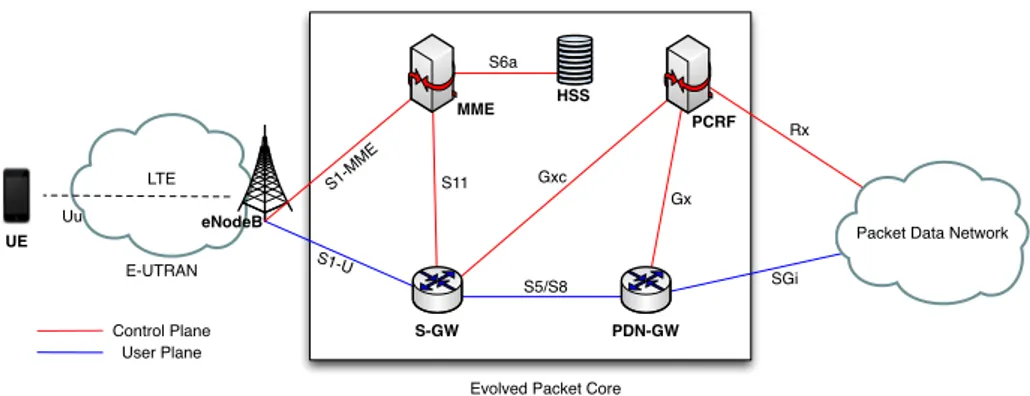
As said before, theEPSis the new network system architecture for enabling data flow to be routed between a mobile terminal and the internet, and vice versa. It includes support for 3GPP radio access technologies (LTE, GSM and WCDMA/HSPA) as well as support for non-3GPP access technologies, the common core of such system is the IPbased network architecture and it is called EPC. The elements related to theEPS are:

• User Equipment (UE): is any device (smart-phone, tablet, notebook or what-ever) that allow the end-user to communicate.

• enhanced NodeB (eNodeB): is the base station to which theUEis connected, it is responsible to manage the radio communication and forward packet to/from the UE.

(8)

• Mobility Management Unit (MME): this device controls the high-level opera-tion of the mobile. It has the ability to track the UEs as they move between cells, and provides bearer management control function to establish the bearer paths that the mobile user will use.

• Serving Gateway (S-GW): routes and forward user data packets, it is an anchor for the UE, means that every flow from/to UE must traverse it. Furthermore it must be selected considering to minimize the probability of changing it when the user change area and eNodeB.

• Packet Data Network Gateway (PDN-GW): it is the EPC’s point of attach to one or more Packet Data Network (PDN). It is assigned to a mobile when it first switches on, to give it always-on connectivity to a default packet data network.

• Home Subscriber Server (HSS): is a central database that contains information about all the network operators subscribers.

As we can see in figure 2.1, all theUEs are connected to a base station eNodeB. The base station is connected to at least one MME over the S1-MME logical interface for the control plane signals. While for the user data payload generated by the UE the eNodeB forward these packets to the S-GW over the S1-U interface. The S-GW forward these data packets to the PDN-GW over the S5 or S8 interface. The first is referred to a communication that is between two gateway of the same Internet Service Provider (ISP), while the second is for the communication where one of the gateway is not in the same ISP’s network. The MME is connected to the HSS over the S6a

(9)

interface. While the SGi interface is used by the PDN-GWto communicate with the external networks PDN. The Uu is the radio interface used for the communication between the UE and the eNodeB. The Policy and Charging Rules Function (PCRF) contains policy control decision and flow-based charging control functionalities. It communicate with the PDN-GW and the S-GW via the Gx and the Gxc interface respectively. The external application servers send and receive service information, for example resource requirementes,IP flow parameters and so on, to thePCRF via the Rx interface.

E-UTRAN LTE

UE

Evolved Packet Core Control Plane User Plane eNodeB S1-MME S1-U S5/S8 S6a SGi Uu HSS MME PCRF

Packet Data Network Gx

Gxc

Rx

S-GW PDN-GW

S11

Figure 2.1: Evolved Packet System

As we can see in 2.1 in the EPC was decided to divide the user plane and the control plane to allow independent scaling for both. The control plane is represented by communication in red, while the data plane is represented by the blue communica-tion. The reason of such choice is that control data signalling tends to scale with the number of users, while user data volumes may scale more dependent on new services and applications.

(10)

2.1.1 Bearer

Data that flows from theUE and the Internet and vice versa, may transport Audio, Video, Gaming etc. For this reason a particular Quality of Service (QoS) must be guaranteed for each on of them. Mobile operator is enabled to use some QoS mecha-nism to privilege treatment of certain users data flows, and at high level the Bearer is a fundamental element related toQoS in theEPS. A Bearer is identified as a virtual path, that flows from the UE to the PDN-GW and vice versa, where all packet that belongs to it experience the same treatment.

E-UTRAN LTE

UE

Evolved Packet Core Control Plane User Plane eNodeB S1-MME S1-U S5/S8 S6a SGi Uu HSS MME PCRF

Packet Data Network Gx Gxc Rx S-GW PDN-GW Radio-Bearer EPS-Bearer S5/S8-Bearer S1-Be arer S11

Figure 2.2: Evolved Packet System Bearer

Since bearer is a virtual path it is mapped into a GPRS Tunnelling Protocol (GTP) Tunnel. This protocol is divided inGTP-U andGTP-C, the former is used for carrying data packet and the latter is for signalling. With this protocol is possible to set up, modify and tear down EPS bearers [9]. The GTP-U protocol carries out a mapping between the S1 and S5/S8 bearers and the fixed network’s transport protocols, by associating each bearer with a bi-directional GTP-U tunnel. In turn, each tunnel is

(11)

associated with two Tunnel Endpoint Identifier (TEID), one for the uplink and one for the downlink. These identifiers are set up using GTP-C signalling messages, and are stored by the network elements 2.3.

UE eNodeB Serving GW PDN GW L1 L2 IP UDP GTP-U PHY MAC RLC PDCP IP UDP/TCP App PHY MAC RLC PDCP L1 L2 IP UDP GTP-U L1 L2 IP UDP GTP-U L1 L2 IP Uu S1-U S5/S8 TEID=17 TEID=5 Radio bearer

Radio bearer TEID=5 TEID=17

Figure 2.3: Protocol Stack

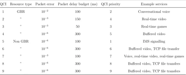
Two important parameter associated to each and every bearer are the following: • Quality of Service Class Identifier (QCI)

• Allocation and Rentention Priority (ARP)

The QCI determines what user plane treatment the IP packets transported on a given bearer should receive, while the ARP specifies the control plane treatment a bearer should receive, this is usually used by the network to decide whether a bearer establishment/modification can be accepted or needs to be rejected due to resource limitations, furthermore it can also be used to decide which existing bearers must be pre-empted during resource limitations. The QCI is an 8-bit number acting as a pointer that refers to a table which defines the same quantities as shown in table 2.1.

(12)

QCI Resource type Packet error Packet delay budget (ms) QCI priority Example services 1 GBR 10 2 ₁₀₀ ₂ _{Conversational voice}

2 ” 10 3 ₁₅₀ ₄ _{Real-time video}

3 ” 10 3 ₅₀ ₃ _{Real-time games}

4 ” 10 6 ₃₀₀ ₅ _{Bu↵ered video}

5 Non GBR 10 6 ₁₀₀ ₁ _{IMS signalling}

6 ” 10 6 ₃₀₀ ₆ _{Bu↵ered video, TCP file transfer}

7 ” 10 3 ₁₀₀ ₇ _{Voice, real-time video, real-time games}

8 ” 10 6 ₃₀₀ ₈ _{Bu↵ered video, TCP file transfers}

9 ” 10 6 ₃₀₀ ₉ _{Bu↵ered video, TCP file transfers}

Table 2.1: QCI table

• Resource Type: indicate whether a bearer has a guaranteed bit rate or not. • Packet delay budget: define an upper bound for the delay that packets sent to

a mobile should experiment.

• QCIpriority: concern with the scheduling process (scheduling weights, admis-sion thresholds,etc.).

• Packet error or loss rate.

The ARP parameter is used to specify the control plane treatment packet a bearer should receive. Furthermore, it is used in resource limitation conditions, in order to decide whether a bearer establishment can be accepted or not. It contains the following parameters:

• priority level is defined as an unsigned 32, is used in situation of resource limita-tion when a bearer could be established or modified only by pre-empting other bearers with lower priority levels.

(13)

• pre-emption capability indicate that a bearer is allowed, or not, to get resources that where assigned to lower priority bearer.

• pre-emption vulnerability specify that a bearer could be pre-empted, or not, by other higher priority bearer.

2.1.2 Gateways Selection

The selection of the gateways is a procedure performed by the MME and is used to select S-GW as well as PDN-GW.

• TheS-GWis selected byMMEat initial attach, this selection is typically based on network topology, the location of theUEwithin the network. Then the best S-GW is selected from a list of ”candidates” that comes out by a procedure called Straightforward Name Authority Pointer (S-NAPTR).

• ThePDN-GWis selected byMMEwhenUEattempts to create a newPDN con-nection or during the initial attach. Usually theUE provides some information like the Access Point Name (APN), or if no such info is provided, theMMEwill use information locate in theHSS.Having those information theMME perform theS-NAPTRprocedure that output a ”candidate” list ofPDN-GW. Then one of those is chosen.

The network that connect those two gateways could have any topology, then, when a S5/S8 Bearer is to be established between an S-GW and aPDN-GW a check must be done to verify that the network has all the needed resources that allow the bearer

(14)

to guarantee its QoS. The purpose of the thesis is to develop some optimization algorithms that allow a flow to be routed and in case of resource limitation the algorithms check if the flow could be routed by pre-empt lower priority flows, otherwise the flow is rejected. The algorithms will be tested in di↵erent load conditions.

2.2 Traffic Engineering

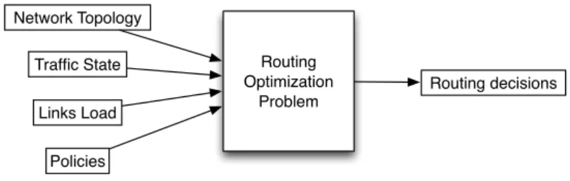
The performance evaluation and performance optimization of operational IP networks are defined as Internet traffic engineering [13]. Reliable network operations is one of the important objective function of the Internet traffic engineering. Then, an important task of the Internet traffic engineering is to control and optimize the routing functions. By correctly managing the traffic through the network and the capacities of the links, the optimization aspects of the traffic engineering can be achieved. This process of managing is not one time goal, but it is continuous and iterative. The traffic engineering, to perform the control of the network, needs to take into account the following information:

• network topology • traffic state • links load • policies

These information are used as input of a optimization routing problem which output will be used to update the routing state 2.4. The routing optimization problem is

(15)

Routing Optimization Problem Network Topology Traffic State Links Load Policies Routing decisions

Figure 2.4: Routing Optimization Problem

mathematically formulated by modelling the network as a directed graph G=(N,A), where N is the set of nodes and A is the set of arcs. Nodes represent the routers, while arcs represent links. Traffic state carry on the information of flows present in the network. Links load represent the residual capacity of links of the network. Then the goal of the optimization problem is to set routes for the demands by finding the optimal path that minimize or maximize a given objective function.

2.3 Related Work

Most of the works related to the EPSare concerned with Selective IP Traffic O✏oad (SIPTO) [6]. For example, in [5] the ”local traffic o✏oad” is used to address non optimal traffic routing in mobile contents distribution and delivery. Other works, instead, deal with an optimal gateway selection [7], to avoid unbalanced load on gateways that will lead to QoS degradation for the users. Work in [1] tackle the problem of routing a flow in a network, under some QoS constraints, but [1] lacks of the concept of priority of flows and thus the pre-emption, and furthermore the networks simulated do not have a structure EPS like. Then we can say that the

(16)

literature lacks of works that take into account at the same time:

• problem of routing a flow under some QoS constraints. • concept of pre-emption.

(17)

Chapter 3 Contribution

3.1 Routing Optimization Algorithms

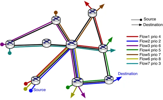
As said in the previous chapter, the purpose of the thesis is to develop some opti-mization algorithms. This algorithms take in input one flow at time and check if is possible to route it, from source to sink, while meeting its constraints. If the flow could not be routed it is not rejected because inEPCeach bearer has the ARPlevel, thus it can do pre-emption/s on other bearers which have lower ARP levels if and only if the resource released allow the flow to be routed, otherwise pre-emption/s will not happen. It is important to specify that when routing a flow and pre-emptions must be performed, than in the subset of lower priority flows the algorithm choose to remove the minimum number of flows and the ones with the lowest priority are preferred. In the simple network in3.1, consider all flows with 80Mbps rate and each link with a capacity of 200Mbps. When the flow #2 must be routed, from Source to

(18)

Destination, resource limitation on the network deny the flow to be routed. Then the flow is not rejected because with pre-emptions it could be routed. In this example the path chosen by flow #2 could be di↵erent, based on the optimization algorithm. Considering the path shown in figure 3.1, the pre-emption will be done over flow #6. It is the minimum number of flows that allow the flow #2 to be routed and between all lower priority flows it is the lowest.

Source Destination Flow1 prio 4 Flow2 prio 2 Flow3 prio 6 Flow4 prio 5 Flow5 prio 7 Flow6 prio 8 Source Destination Flow7 prio 3

Figure 3.1: Pre-emption Example

As said, the behaviour of the three optimization algorithms is di↵erent. The following is a detailed description for each one of them.

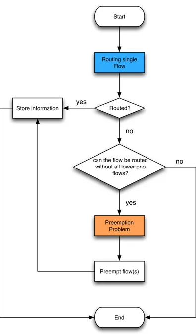
Algorithm 1 (3.2) When a flow has to be routed the algorithm check if it is possible to route it, if is not possible another try is done, but this time the computation is

(19)

done by removing all the lower priority flows that traverse the network, then if a path that meets the QoS constraints exist, a pre-emption problem is set up to minimize the number flows that must be pre-empted, otherwise the flow is rejected. In this optimization algorithm the QoS comes first than the pre-emption. When pre-emptions must be done in order to allow the flow to be routed, it first search for a path that satisfy the QoS constraints and then try to reduce the number of flows to pre-empt on that given path.

(20)

Start

Routing single Flow

Routed?

Store information yes

no

can the flow be routed without all lower prio

flows? yes Preemption Problem Preempt flow(s) End no

Figure 3.2: Optimization Problem 1

Algorithm 2 (3.3) When a flow has to be routed the algorithm check if it is possible to route it and, if is not possible, another try is done, but this time the

(21)

computation is done step by step. The priority ’P’ is set up to the lowest and then all the flows with this priority will be removed, then if the flow could be routed a problem is set up to minimize the number of flow to remove. Otherwise the priority ’P’ is incremented by a unit and then all flows with a priority equal than ’P’ are removed (in addition to the flows that were previously removed the step before) and then if the flow could be routed a pre-emption problem is set up. The procedure continue until the priority ’P’ is one unit less the priority of the flow the must be routed, if no path is found during these steps the flow will be rejected. Even in this optimization algorithm, when pre-emptions must be done, first search for a path that satisfy the QoS constraints and then try to reduce the number of flows to pre-empt on that given path. Di↵erent than the algorithm OP11 (3.2) there is a time overhead due to the level-by-level searching of the set of flows to pre-empt that allow the flow to be routed.

(22)

Start

Routed?

Store information yes

no

can the flow be routed without X prio flows??

yes Preempt flow(s) End X = Lowest Priority Increment X priority is X = Y yes no no Routing single Flow of Y priority Preemption Problem

(23)

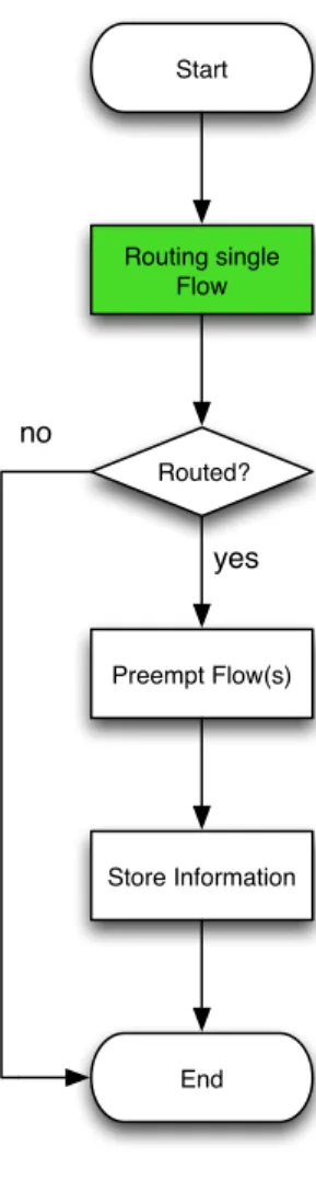
Algorithm 3 (3.4) When a flow has to be routed the algorithm set up a problem that check if it is possible to route it in the network by choosing the path that at the same time meets the QoS constraints and minimize the number of pre-emptions, otherwise the flow cannot be routed and it is rejected. In this optimization algorithm, whether pre-emptions must be done or not, the search for a path is done by considering jointly QoS constraints and pre-emptions.

Start Routing single Flow Routed? Preempt Flow(s) Store Information End yes no

(24)

3.2 Mathematical Formulations

Routing a flow with a given rate ⇢ and burst , from a source to a destination within a end-to-end delay, in a network, is a routing optimization problem. The network is modelled as a directed graph G = (N,A), where N is the set of nodes, corresponding to the routers in the network, and A is the set of directed arcs, corresponding to the links in the network. To solve this problem it was used a tool for path computation [1] that set and solve a routing optimization problem, of which will be shown only the objective function and some constraints of interest.

min X

(i,j)2A

fi,j⇤ ri,j

3.1: Base Objective Function

X (j,i)2BS(i) xj,i X (i,j)2F S(i) xi,j = 8 > > > > > > < > > > > > > : 1 if i = s 1 if i = d 0 otherwise ⇢_{⇤ x}ij  rij  cij ⇤ xij (i, j)2 A

3.2: Flow Conservation Constraint

• xi,j is a binary variable that indicate whether link (i,j) belongs to the path.

• ri,j is a variable that represents the rate allocated to the link (i,j).

(25)

• ci,j is a variable that represent the capacity of the link (i,j).

First constraint is for the flow conservation, the second, instead, is the rates con-straint, so each rate allocated must be bounded within ⇢ and the capacity of the link the rate is being allocated. This type of routing optimization problem takes in input the network with the all information related and return, if the flow could be routed, the path that the flow will follow and the rates allocated to the flow in the links of the path. The routing optimization problem partially shown above is the blue one process in the routing optimization algorithms represented in figures 3.2 and 3.3. In both of the routing optimization algorithms 3.2 and 3.3, there is another process coloured as orange. This routing optimization problem is set up when pre-emption must be done in order to allow the flow to be routed. Consider that the path of the flows was previously chosen and then in that path the goal of the problem is to minimize the number of flows to pre-empt. The problem is shown as follows:

min X

(i,j)2A

pk⇤ ak

3.3: Pre-emption Problem Objective Function

rij + X m2HP F lows rm_ij + X n2LP F lows rn_ij X k2LP F lows r_ijk ⇤ ak  wij (i, j)2 P ath 3.4: Pre-emption Constraint

(26)

• ai is a binary variable that indicate whether a flow must be pre-empted or not.

• HPFlows is the set of higher priority flows • LPFlows is the set of lower priority flows

• ri,j is a variable that represents the rate allocated to the link (i,j)

• ci,j is a variable that represent the capacity of the link (i,j)

• pk is the weight assigned to the flows in relations of their priorities.

Last one routing optimization problem is used in the routing optimization algo-rithms shown in 3.4. Rather than the other algorithms in this one there is only one process representing a routing optimization problem. The objective function is com-posed by two distinct parts, the first concerns with the rate allocations while the second is relative to the pre-emptions. The overall goal of this problem is to minimize the rate allocation and minimize the pre-emptions, if any, to do in order to allow the flow to be routed. In this case the in the moment of routing a flow the problem consider the path that guarantee the QoS needed by the flow and that minimize the pre-emptions, or not to do them at all. Objective function and some constrains are shown below: min X (i,j)2A fi,j ⇤ ri,j + w⇤ X k2F lows pk⇤ ak

(27)

⇢_{⇤ x}ij  rij  (wij

X

k2HigherP riorityflows

r_ijk)_{⇤ x}ij (i, j)2 A

3.6: Rate Constraint Optimization Problem 3

rij + X m2HP F lows rm_ij + X n2LP F lows rn_ij X l2LP F lows r_ijl _{⇤ a}l  wij (i, j)2 P ath

3.7: Pre-emption Constraint Optimization Problem 3

• ai is a binary variable that indicate whether a flow must be pre-empted or not.

• w is the weight assigned to the second part of the objective function, in order to make it more or less incisive in the choosing of the path.

• pk is the weight assigned to the flows in relations of their priorities.

• xi,j is a binary variable that indicate whether link (i,j) belongs to the path.

• ri,j is a variable that represents the rate allocated to the link (i,j)

• fi,j is a weight for the rates in the objective function.

• ci,j is a variable that represent the capacity of the link (i,j)

• HPFlows is the set of higher priority flows • LPFlows is the set of lower priority flows

(28)

In the rate constraint 3.6 we specify that the rate allocated to the flow at each link of the path must be bounded within ⇢ that is the minimum rate, and the capacity of the link. This one must be considered as the total capacity less the rates of higher priority flows (they cannot be pre-empted). With the second constraint3.7 if for the pre-emption.

3.3 CPLEX

To solve all problems previously shown the tool used is provided by International Business Machines (IBM), it is the IBM ILOG CPLEX Optimization Studio [2]. This software allows the user to set up a problem, solve it and get the results. IBM [2] o↵ers a number of interfaces for building and deploying optimization applications using all of the IBM ILOG CPLEX Optimizers:

3.3.1 What is CPLEX

IBM ILOG CPLEX Optimization Studio and the embedded IBM ILOG CPLEX CP Optimizer constraint programming engine provide serialized keywords and syntax for modelling detailed scheduling problems. It o↵ers C, C++, Java, .NET, and Python libraries that solve Linear Programming (LP) and related problems. Specifically, it solves linearly or quadratically constrained optimization problems where the objective to be optimized can be expressed as a linear function or a convex quadratic function. CPLEX comes in these forms to meet a wide range of users needs:

(29)

• The CPLEX Interactive Optimizer: is a command-line interactive program, provided in executable, ready-to-use form. It can read the problem interactively or from a file, issue the ”optimize” command to solve the problem, and then deliver the solution interactively or into a file.

• Concert Technology: is a set of libraries developed for three di↵erent lan-guage, C++, Java and .Net. Concert Technology can be used to model, write customized optimization algorithms (based on the provided ones) and embed the created models and algorithms into an application

• The CPLEX Callable Library: is a matrix-oriented library with a C pro-gramming language interface for the ILOG CPLEX Optimizer. This interface provides all the features of the Callable Library without the need to manage lengths of arrays, allocation of memory and freeing of memory.With this library the programmer can embed ILOG CPLEX Optimizer optimizers in applications written in C, Visual Basic, FORTRAN, CPP and so on.

(30)

3.3.2 Callable Library Component

In this thesis the CPLEX Callable Library was used, it allows developers to effi-ciently embed IBM ILOG optimization technology directly in the applications. A comprehensive set of routines is included for defining, solving, analysing, querying and creating reports for optimization problems and solutions. The structure of this library is shown in figure 3.5. The Callable Library itself contains routines divided into several categories:

• problem modification routines let the user define a problem and change it after its creation.

• optimization routines enable the user to optimize a problem and generate re-sults.

• utility routines handle application programming issues.

• problem query routines access information about a problem after you have cre-ated it.

• file reading and writing routines move information from the file system of oper-ating system into user application, or from user application into the file system.

• parameter routines enable the user to query, set, or modify parameter values maintained by CPLEX.

(31)

User Written Application

CPLEX Callable Library

CPLEX Internals

Figure 3.5: CPLEX Callable Library

3.3.3 Example of use

Here are some lines of code that specify how to set up a problem, solve it and get the results. Begin with the setting up of the CPLEX environment:

env = CPXopenCPLEX(& s t a t u s ) ;

l p = CPXcreateprob ( env , &s t a t u s , " CPLEX_PROBLEM_NAME " ) ; CPXchgobjsen ( env , lp , CPX MIN) ;

Listing 3.1: CPLEX set up

With the CPXopenCPLEX we initialize the environment that will host the CPLEX problem. The CPXcreateprob routine specifies to create an empty CPLEX problem, and then with the CPXchgobjsen routine we specify the type of objective function, i.e. min.

(32)

int i , s t a t u s , c c n t = n u m v a r i a b l e s ;

double _{⇤ obj , ⇤ lb , ⇤ub ;}

char _{⇤⇤vnames = 0 , ⇤ ctype ;}

o b j = new double [ c c n t ] ; l b = new double [ c c n t ] ; ub = new double [ c c n t ] ; c t y p e = new char [ c c n t ] ;

vnames = new char_{⇤ [ ccnt ] ;}

f o r ( i = 0 ; i < c c n t ; i ++) vnames [ i ] = new char [ 1 0 ] ;

f o r ( i = 0 ; i < n u m v a r i a b l e s ; i ++) _{ l b [ i ] = 0 ; ub [ i ] = 1 ; o b j [ i ] = 1 ; c t y p e [ i ] = ’B’ ; s p r i n t f ( vnames [ i ] , " name_ %d" , i ) ; }

s t a t u s = CPXnewcols ( env , lp , ccnt , obj , lb , ub , ctype , vnames ) ;

Listing 3.2: add CPLEX columns

Now we have just specified to CPLEX which variables we want in our problem and: • Lower bound and Upper bound of each variable.

• Which ones go in the objective function and their relative coefficients. • Name for each variable.

• Type of each variables (i.e. ’B’ stands for binary).

We are almost done with the set up of the problem. Now we have to specify the con-strains of our problem, the following lines of code represent how to add one constraint

(33)

to the CPLEX problem:

r c n t = 1 ;

rmatbeg = new int [ 1 ] ; r h s = new double [ 1 ] ; s e n s e = new char [ 1 ] ; rmatbeg [ 0 ] = 0 ; s e n s e [ 0 ] = ’G’ ;

n z c n t = n u m o f n o n z e r o c o e f f ; rmatind = new int [ n z c n t ] ; rmatval = new double [ n z c n t ] ;

f o r ( int f l o w = 0 ; f l o w < n u m o f n o n z e r o c o e f f ; f l o w++) { rmatind [ f l o w ] = i n d e x o f t h e v a r i a b l e ; rmatval [ f l o w ] = c o e f f i c i e n t o f t h e v a r i a b l e ; } r h s [ 0 ] = 0 . 0 ; s t a t u s = CPXaddrows ( env , lp , 0 , r c n t , nzcnt , rhs , s e n s e , rmatbeg , rmatind , rmatval , NULL, NULL) ;

Listing 3.3: add constraint

With the routine CPXaddrows all the constraints are stored sequentially in the arrays rmatbeg, rmatind, rmatval.

• rmatbeg specify where each row begin.

• rmatind specify the column index of the variables which go in the constraints. • rmatval specify the coefficient for each variables specified in rmatind.

• rcnt is an integer that indicates the number of new rows to be added to the constraint matrix.

(34)

• nzcnt is an integer that indicates the number of non-zero coefficient to be added to the constraint matrix.

• rhs is an array that contain the right hand side coefficient of each constraint. • sense is an array that specifies the type of constraint (G is , L is , E is =). In the code shown above we added only one constraints. We have set the rows counter to 1. Problem set up, now we have to solve it and get the results:

s t a t u s = CPXmipopt ( env , l p ) ;

double ⇤ x = new double [ nu m vari ables ] ;

s t a t u s = CPXgetx ( env , lp , x , 0 , n u m v a r i a b l e s 1) ;

Listing 3.4: solve and get results

Our problem was a mixed integer then we used the CPXmipopt routine to solve it. After solving the problem we get the result array with the CPXgetx routine.

(35)

3.4 Network Topologies

No information known about the actual network topologies between theS-GWs and the PDN-GWs have led us to generate some own topologies. We referred to real topologies provided by The Internet Topology Zoo [3] and then we processed those topologies to make them more likely theEPSnetworks. The first part of parsing was done according of the set-up in [1] where the Fast Network Simulation Setup (FNSS) tool was used [4], in this part the delays and the capacities to the links of the networks were assigned. Then, having a network topology modelled as a graph, the second part of the parsing took place as follows:

• seletc the PDN-GWs • select the S-GWs

• Adding nodes to the topology, acting as eNodeBs attached to the S-GWs • Flows generation (source,destination,deadline)

In the PDN-GWs selections a scan of every node is done and only the nodes with the max incoming degree are selected to be a PDN-GW. Then the remaining nodes are scanned and each node could be selected as an S-GW with a probability that is inversely proportional to the out-coming degree of the node itself (3.8). Furthermore, to ensure that the S-GWs are as much as possible distant from the PDN-GWs, the S-GWs are selected to be at least two hop distance form the nearest PDN-GW.

(36)

pnodei =

1 degreenodei

3.8: S-GW selection probability

Clearly if the degree is 1 the node is selected as an S-GW for sure. Last topology phase was to attach theeNodeB to theS-GWs, with an uplink and a downlink. The figure3.6 show the graphical result of what just said.

(37)

Last node added to the network topologies is the so called Super Node [3.7]. Somehow it represents the Internet that each flow, originated by a UE, is trying to reach. It is directly connected to all thePDN-GW. These links have a null delay and infinite capacity. Having said that, from the routing perspective the choice of one or anotherPDN-GW, in order to reach it, is driven only by the network load. With this trick we are implicitly balancing network load.

EPC PDN-GW PDN-GW PDN-GW Super Node ,0 ,0 ,0 (capacity,delay)

Figure 3.7: Super Node

3.5 Flow generations

The flows generation consist of several phases and the info related to the flows are the following:

• Source. • Destination. • Rate.

(38)

• Burst. • Deadline.

Considering that the source of each flow is the UE, but we have not considered the radio bearer in this thesis, we have set the eNodeBs as the source of each flow. The destination was, instead, the Packet Data Network, represented by the Super Node. The Super Node, as said before, have allowed us to balance the load on the network. Flows generated were uniformly distributed on the eNodeBs present in the network. Rates ⇢ were uniformly generated within a range of values [80, 160]M bps. The burst was fixed and its value was = 3⇤ MT U. The deadline was generated within a interval defined by an upper bound and a lower bound. The upper bound was defined as the max delay that a packet could experience traversing the path from source to destination. In the same path from source to destination the minimum delay experienced is the lower bound. The path from source to destination was calculated using the Dijkstra’s algorithm [10]. Then we calculated the delay from source to destination by using the shortest path given by Dijkstra. In every single link we calculated the delay in two di↵erent ways, one is referred to the upper bound and one for the lower bound:

delaylbi,j =

capacityi,j

delayubi,j =

⇢ 3.9: Delay calculation

In figure 3.8 the algorithm starts from node 1 and choose the next node on a distance base in order to reach the destination with the minimum hop. The delay is

(39)

step by step cumulated and at the end of the algorithm we have calculated the lower bound and upper bound as shown in 3.10:

Source

Destination

capacity(i,j)

j i

Figure 3.8: Deadline Calculation in Shortest Path

lowerbound = X

(linki,j2P athcapacityi,j

upperbound = X

(linki,j)2P ath ⇢

3.10: Upper and lower bound formula

Clearly, delay requests smaller than the lower bound cannot be met, while requests higher than the upper bound are more likely to make the delay constraint redundant. For the random generation we used the rand() function of C++ Standard Library. It returns a pseudo-random integral number in the range between 0 and RANDMAX. Then we generate a delta (3.11) bounded in the interval [0, U pperbound Lowerbound] and then we sum it to the lower bound delay.

(40)

delta = rand()

RAN DM AX ⇤ (Upperbound Lowerbound) 3.11: Delta Calculation

3.6 Simulator

The main task of the simulator is to generate the arrivals and departures of flows in the network. It handles the generation of inputs for the optimization algorithms. An input for the optimization algorithms means that a new flows has arrived and must be routed. Furthermore the simulator has also the task of removing flows from the network, which represent a departure of a flow.

(41)

Simulator Optimization Algorithm Network State R O U T E U P D A T E [Flow Arrival] [Flow Departure] R O U T E U P D A T E [Flow Arrival] [Flow Departure] U P D A T E U P D A T E = arrival rate = departure rate

Figure 3.9: Simulator Diagram

The sequence diagram of figure 3.9 show how the simulator works. The flow arrivals are generated at time intervals exponentially distributed, with a varying rate . Flows are all numbered from 1 to NUM MAX, and then a random function is used to generate the index of the flow to be the new one arrived. Furthermore is the flow index just generated correspond to a flow that is still in the network, a new one index is generated. A flow in the network last for an exponentially distributed time with

(42)

a mean equal to 1 second. If the flow just arrived has been routed correctly the floe departure event is generated, otherwise it is not generated. In any case at the same time of the flow arrival event, the next flow arrival event is generated. Defined as the arrival rate and µ as the departure rate, we can then define the load of the network as follows: _µ. As we want to study how the networks respond as the load vary we fixed the value of µ to 1 and then we varied the arrival rate to simulate networks in di↵erent load conditions. The simulation time was calculated as following:

5 ⇤ max{nflows, 1 Pmin} where Pmin = 8 > > < > > : 10 2 _if _{> 5} 10 3 _otherwise

Which yields enough sample to correctly estimate blocking probability, average time of routing and pre-emption ratio. The simulation of the di↵erent networks in di↵erent load conditions was repeated three time in order to have an average value.

3.7 Optimization Algorithms Calibration

3.7.1 Pre-emption Problem Calibration

The pre-emption problem objective function shown in3.3 presents coefficients pk that

represent the weight assigned to each flow on a priority basis. Then, as said in [8], we related the priority level with the weight with a linear function. In our case we used the priority of bearers which values goes from 1 to 15. A value of 1 is the highest priority level, while 15 is the lowest priority level. The function is the following:

(43)

For example a flow which has a priority of 5 will have a weight of 11, while a flow which has a priority of 10 will have a weight of 6.

3.7.2 Optimization Problem 3 Calibration

As shown in formula 3.5 the objective function is composed by two parts. In the first part the goal is to minimize the rate allocated, during the path, to the flow that must be routed. While in the second part the goal is to minimize the number of pre-emptions that must be done in order to allow the flow to be routed. We decided to make more important the second part of the objective function by assign a weight of 1 to the first and a weight much bigger to the second part (the w coefficient). While for the pk coefficient holds the same criteria of section 3.7.1. We have tested

the optimization algorithm three with di↵erent weights _{{10; 10}3_{; 10}6_{; 10}9_{} and then}

we have chosen the one who showed the best behaviour as for:

• Blocking probability: represent the probability of a flow rejection.

• Pre-emption ratio: is the fraction of flow pre-empted out of the total number of flow handled.

• Average time: is referred to the mean time the algorithm need to route or reject a new flow arrival.

Tests were done with the following networks:

(44)

• Intellifiber (3.12). • Iris (3.14).

• Cernet (3.16).

As we can see in the plots of pre-emption ratio in 3.11,3.13,3.15 and 3.17, the smaller the weight is the more pre-emptions will be done. This behaviour is completely reflected in the blocking probability, indeed we can say that the more pre-emptions done the less blocking probability is. Furthermore the behaviours with the weights 103_{, 10}6 _{and 10}9 _{are quite identical as for blocking probability and pre-emption ratio.}

The trend of average time plots is that the smaller the weight is the more average time is needed by the routing algorithm. The choice of the weights is between 106

and 109_{, and we have chosen the 10}6 _{because its behaviour is quite identical to the}

weight 109 _{as for blocking probability and for pre-emption ratio. It is very similar}

for the average time, but it allows us to do not unbalance too much the objective function.

(45)

(46)

0 500 1000 1500 2000 2500 3000 3500 4000 0 0.2 0.4 0.6 0.8 Renater2010 lambda Blocking Probability w = 1e9 w = 1e6 w= 1e3 w = 1e1 0 500 1000 1500 2000 2500 3000 3500 4000 0 0.1 0.2 0.3 0.4 Renater2010 lambda Preemption Ratio w = 1e9 w = 1e6 w= 1e3 w = 1e1 0 500 1000 1500 2000 2500 3000 3500 4000 0.2 0.3 0.4 0.5 0.6 0.7 Renater2010 lambda Average Time w = 1e9 w = 1e6 w= 1e3 w = 1e1

(47)

(48)

0 500 1000 1500 2000 2500 3000 3500 4000 0 0.2 0.4 0.6 0.8 Intellifiber lambda Blocking Probability w = 1e9 w = 1e6 w= 1e3 w = 1e1 0 500 1000 1500 2000 2500 3000 3500 4000 0 0.1 0.2 0.3 0.4 Intellifiber lambda Preemption Ratio w = 1e9 w = 1e6 w= 1e3 w = 1e1 0 500 1000 1500 2000 2500 3000 3500 4000 0.2 0.4 0.6 0.8 1 Intellifiber lambda Average Time w = 1e9 w = 1e6 w= 1e3 w = 1e1

(49)

(50)

0 500 1000 1500 2000 2500 3000 3500 4000 0 0.2 0.4 0.6 0.8 Iris lambda Blocking Probability w = 1e9 w = 1e6 w= 1e3 w = 1e1 0 500 1000 1500 2000 2500 3000 3500 4000 0 0.1 0.2 0.3 0.4 Iris lambda Preemption Ratio w = 1e9 w = 1e6 w= 1e3 w = 1e1 0 500 1000 1500 2000 2500 3000 3500 4000 0.2 0.4 0.6 0.8 1 Iris lambda Average Time w = 1e9 w = 1e6 w= 1e3 w = 1e1

(51)

(52)

0 500 1000 1500 2000 2500 3000 3500 4000 0 0.2 0.4 0.6 0.8 Cernet lambda Blocking Probability w = 1e9 w = 1e6 w= 1e3 w = 1e1 0 500 1000 1500 2000 2500 3000 3500 4000 0 0.1 0.2 0.3 0.4 Cernet lambda Preemption Ratio w = 1e9 w = 1e6 w= 1e3 w = 1e1 0 500 1000 1500 2000 2500 3000 3500 4000 0.1 0.2 0.3 0.4 0.5 Cernet lambda Average Time w = 1e9 w = 1e6 w= 1e3 w = 1e1

(53)

Chapter 4 Performance Evaluation

In this chapter we will present the results of our simulations. The networks that have been simulated are the following:

• Renater (3.10). • Iris (3.14).

• Intellifiber (3.12). • Cernet (3.16).

In the table 4.1 are shown some characteristics of these networks, i.e. number of nodes, number of links and so on. Considering the number of nodes the simplest network is the Cernet, while the Intellifiber is the one with the maximum number of nodes. The number of nodes is strictly related to the number of links. The same consideration could be done for the number of links, because the number of links is

(54)

strictly proportional to the number of nodes, then the Cernet is always the simplest network and the Intellifiber is the one with the maximum number of links. The number of PDN-GW was chosen considering that too much will have reduced the number of S-GW and too less (i.e. one) would be not sufficient to our experiments. Then we chosen to select three PDN-GWs per network.

Topology # nodes #PDN-GW #S-GW #eNodeBperS-GW # links # flows avg. node rank avg. prop. delay avg. flow deadline

Cernet 77 3 7 5 192 5000 2,41 3,95 9,86

Renater2010 109 ” 13 ” 248 ” 2,22 3,06 9,82

Iris 147 ” 19 ” 324 ” 2,16 10 4,881

Intellifiber 259 ” 37 ” 566 ” 2,18 2,28 8,76

Table 4.1: Topologies characteristics

The flow characteristics are shown in table 4.2, the sources of flows are the eNodeBs, while the destinations are all the same and it is the Super Node. Rate of flows was randomly generated within the interval [80,160]Mbps , while the burst was fixed to 4500 byte that correspond to 3 times the Maximum Transmission Unit (MTU). The priority are randomly generated within 1 and 15. The first is the higher priority level while the second is the lowest.

Source eNodeB

Destination Super Node Rate [Mbps] [80,160] Burst [Byte] 4500

Priority [1,15] Table 4.2: Flows characteristics

(55)

The metrics that we are going to show for the chosen networks are the following:

• Blocking Probability. • Pre-emption Ratio.

• Average Computation Time.

Some common behaviours of the three optimization algorithms are quite evident in all the networks simulated. The pre-emptions rise until it’s reached an high rejection rate, then it begins to fall due to the blocking probability rising. The Blocking probability is always rising, more aggressive at lower , and more smoothed at higher . For the average time we need to say that routing a flow take more time than reject it. Having said that , the more time is needed by the optimization algorithms the lower lambda and blocking probability is. When the blocking probability rise the flows rejections are more and then the average time falls.

4.0.3 Renater

In the plots of the Renater4.1 we can see that the blocking probability is quite identi-cal as for OP12 (3.3) and OP3 (3.4), and quite similar for the OP11 (3.2). This is due to the pre-emption ratio, in this plot we see that the OP3 (3.4) is the one who makes less pre-emptions, while the OP11 (3.2) and OP12 (3.3) make approximately the same number of pre-emptions. The OP3 (3.4) is the one who make less preemptions because it choose the best path from source to destination that reduce the number of pre-emptions while meeting the QoS constraints. The other two don’t have this

(56)

concept and then they make the minimum pre-emptions as possible on a given path chosen with the only concept of satisfying the QoS constraints. Another considera-tion about the relaconsidera-tion between pre-empconsidera-tion and blocking probability is that even if the the OP3 (3.4) and the OP12 (3.3) have di↵erent pre-emption ratio curves, their blocking probability are quite identical, and this is explained by the fact that they work hard on the lowest priority flows. This means that they leave in the network the higher priority flows and then when a new flow arrives it is higher the probability of rejection. The average time plot show that the OP11 (3.2) is the simplest one. The other two are more expensive, until = 1500 is better remove level-by-level priority flows instead of set up the problem considering jointly the QoS and the pre-emptions. After that lambda the behaviours exchange, this is due to the high rejection of flows, indeed try to remove flows level-by-level is good-for-nothing when a flow has to be rejected and take more time than the OP3 (3.4).

(57)

0 500 1000 1500 2000 2500 3000 3500 4000 4500 0 0.2 0.4 0.6 0.8 lambda blocking probability Renater2010BlocProb−ro[80,160]−sigma36000−5eNB−3pgw−5000flows−5runs OP11 OP12 OP3 0 500 1000 1500 2000 2500 3000 3500 4000 4500 0 0.1 0.2 0.3 0.4 lambda preemption ratio Renater2010PreeRatio−ro[80,160]−sigma36000−5eNB−3pgw−5000flows−5runs OP11 OP12 OP3 0 500 1000 1500 2000 2500 3000 3500 4000 4500 0 0.5 1 1.5 2 2.5 lambda average times Renater2010AvgTimes−ro[80,160]−sigma36000−5eNB−3pgw−5000flows−5runs OP11 OP12 OP3

Figure 4.1: Renater network simulations

4.0.4 Iris

In Iris plots 4.2 the OP3 (3.4) still is the one algorithm that makes less pre-emptions than the other two. Less pre-emptions means that the blocking probability is high. Even for the OP12 (3.3) the blocking probability is high, and this is because the pre-emptions done, are all done by removing the lower priority flows and then when a new flow arrive it is more likelihood to be rejected. The algorithm OP11 (3.2) is the one who make more pre-emptions and has the lowest blocking probability. In this

(58)

network we can also see that the average time needed for the computing is higher than the Renater4.1. This is due to the network type (4.1) that has more links than Renater. The algorithm OP12 (3.3) is the more a↵ected one by this characteristics.

0 500 1000 1500 2000 2500 3000 3500 4000 4500 0 0.2 0.4 0.6 0.8 lambda blocking probability IrisBlocProb−ro[80,160]−sigma36000−5eNB−3pgw−5000flows−5runs OP11 OP12 OP3 0 500 1000 1500 2000 2500 3000 3500 4000 4500 0 0.1 0.2 0.3 0.4 lambda preemption ratio IrisPreeRatio−ro[80,160]−sigma36000−5eNB−3pgw−5000flows−5runs OP11 OP12 OP3 0 500 1000 1500 2000 2500 3000 3500 4000 4500 0 1 2 3 4 lambda average times IrisAvgTimes−ro[80,160]−sigma36000−5eNB−3pgw−5000flows−5runs OP11 OP12 OP3

Figure 4.2: Iris network simulations

4.0.5 Cernet

The Cernet network as we can see in the table 4.1, this is the simplest network. Indeed we can see that the blocking probability rises slower than the other networks simulated. To reach the 20% of the blocking probaiblity the arrival rate must be 1000

(59)

flows per second, while in the other networks it is just 500. Di↵erences between the optimization algorithms still holds even in this network. The OP11 (3.2) is still the one with the lower blocking probability. This behaviour is due to the pre-emption ratio, indeed the OP11 (3.2) is the one who make more pre-emptions than the other two. The OP12 (3.3) and the OP3 (3.4) even if they make less pre-emptions they have an higher blocking probability due to the incisive removing of lower priority flows. This make more probably that a lower priority flows, that comes after, will be rejected. Last plots in 4.3 show that the average time, in this simple network, is the same for all of three algorithms, and it is less then the time required in the other networks. The more time is needed when the rate of arrival flows is lower and it falls when the arrival flows rate rises.

(60)

0 500 1000 1500 2000 2500 3000 3500 4000 4500 0 0.2 0.4 0.6 0.8 lambda blocking probability CernetBlocProb−ro[80,160]−sigma36000−5eNB−3pgw−5000flows−5runs OP11 OP12 OP3 0 500 1000 1500 2000 2500 3000 3500 4000 4500 0 0.1 0.2 0.3 0.4 lambda preemption ratio CernetPreeRatio−ro[80,160]−sigma36000−5eNB−3pgw−5000flows−5runs OP11 OP12 OP3 0 500 1000 1500 2000 2500 3000 3500 4000 4500 −0.5 0 0.5 1 1.5 2 lambda average times CernetAvgTimes−ro[80,160]−sigma36000−5eNB−3pgw−5000flows−5runs OP11 OP12 OP3

Figure 4.3: Cernet network simulations

4.0.6 Intellifiber

The same considerations could be done for the intellifiber network, as for blocking probability and pre-emption ratio. The first is alway rising and the three optimization algorithm have the same behaviour. The second is rising until is reached an high rejecting rate and then it is falling. Even in this network the OP11 (3.2) blocking probability is a bit lower than the other two. As for the other networks, the pre-emption ratio is the lowest for the OP3 (3.4). This network show us a particular

(61)

behaviour in the average time of the OP12 (3.3). When the lambda rises and the rejection is high the algorithm show that going level-by-level for the pre-emptionS is e↵ortless (because most of times the flow cannot be routed anyway) and the time needed is higher than the other two algorithms.

0 500 1000 1500 2000 2500 3000 3500 4000 4500 0 0.2 0.4 0.6 0.8 lambda blocking probability IntellifiberBlocProb−ro[80,160]−sigma36000−5eNB−3pgw−5000flows−5runs OP11 OP12 OP3 0 500 1000 1500 2000 2500 3000 3500 4000 4500 0.05 0.1 0.15 0.2 0.25 0.3 lambda preemption ratio IntellifiberPreeRatio−ro[80,160]−sigma36000−5eNB−3pgw−5000flows−5runs OP11 OP12 OP3 0 500 1000 1500 2000 2500 3000 3500 4000 4500 0 2 4 6 8 lambda average times IntellifiberAvgTimes−ro[80,160]−sigma36000−5eNB−3pgw−5000flows−5runs OP11 OP12 OP3

(62)

(63)

Chapter 5 Conclusions

In this thesis the problem of optimal joint path computation and resource alloca-tion policies in EPCnetworks has been addressed. We have tested the three routing optimization models in realistic networks as for blocking probability, pre-emption probability and time overhead. Our results show that the algorithms exhibits similar behaviours as for blocking and pre-emption probability. Time needed for the compu-tations are di↵erent, depending on the network and the optimization problem. The more links and nodes are in the network, the more average time is needed. More-over, blocking and pre-emption seem to be contrasting goals: one is reduced at the expenses of the other. As for time overhead, computations on o↵-the-shelf hardware show that an optimization approach is compatible with a highly-dynamic large-scale environment.

(64)

(65)

Chapter 6 Acknowledgements

I would like to o↵er my special thanks to Engineer Giovanni Stea , my supervisor, and Professor Antonio Frangioni for giving me the opportunity to deal with the topics of this thesis. Their useful comments, remarks and engagements helped me to going through the learning process of this master thesis. My grateful thanks to Engineer Antonio Virdis and Engineer Laura Galli for their valuable and constructive suggestions during the planning and development of this research work. Their advices were of fundamental importance to complete this master thesis. I wish to thank all the guys of the PerLab and RedLab, who accompanied me during this months. A special thank to the old friends in Messina, and the new ones in Pisa. I’d like to thank all the friends that I met during these years. A special thank to all my family, without them would not have been possible to achieve this goal. Words cannot express how grateful I am to them for all the sacrifices that they made on my behalf.

(66)

(67)

Chapter 7 Acronyms

ARP Allocation and Rentention Priority EPC Evolved Packet Core

EPS Evolved Packet System

E-UTRAN Evolved Universal Terrestrial Access Network EPS Evolved Packet System

PDN-GW Packet Data Network Gateway QoS Quality of Service

QCI Quality of Service Class Identifier S-GW Serving Gateway

UE User Equipment

(68)

S-NAPTR Straightforward Name Authority Pointer ISP Internet Service Provider

LTE Long Term Evolution

3GPP 3rd Generation Partnership Project IP Internet Protocol

MME Mobility Management Unit PDN Packet Data Network

ISPs Internet Service Providers eNodeB enhanced NodeB HSS Home Subscriber Server

IBM International Business Machines FNSS Fast Network Simulation Setup SIPTO Selective IP Traffic O✏oad GTP GPRS Tunnelling Protocol GPRS General Packet Radio Service TEID Tunnel Endpoint Identifier APN Access Point Name

(69)

MTU Maximum Transmission Unit

PCRF Policy and Charging Rules Function IP Internet Protocol

(70)

(71)

List of Figures

2.1 Evolved Packet System . . . 9

2.2 Evolved Packet System Bearer . . . 10

2.3 Protocol Stack . . . 11

2.4 Routing Optimization Problem . . . 15

3.1 Pre-emption Example . . . 18

3.2 Optimization Problem 1 . . . 20

3.5 CPLEX Callable Library . . . 31

3.6 Example of a Simple Parsed Topology . . . 36

3.7 Super Node . . . 37

3.8 Deadline Calculation in Shortest Path . . . 39

3.9 Simulator Diagram . . . 41 71

(72)

3.10 Renater 2010 . . . 45 3.11 Renater 2010 Calibration . . . 46 3.12 Intellifiber . . . 47 3.13 Intellifiber Calibration . . . 48 3.14 Iris . . . 49 3.15 Iris Calibration . . . 50 3.16 Cernet . . . 51 3.17 Cernet Calibration . . . 52

4.1 Renater network simulations . . . 57

4.2 Iris network simulations . . . 58

4.3 Cernet network simulations . . . 60

(73)

Listings

3.1 CPLEX set up . . . 31

3.2 add CPLEX columns . . . 32

3.3 add constraint . . . 33

3.4 solve and get results . . . 34

(74)

(75)

List of equations

3.1 Base Objective Function . . . 24

3.2 Flow Conservation Constraint . . . 24

3.3 Pre-emption Problem Objective Function . . . 25

3.4 Pre-emption Constraint . . . 25

3.5 Objective Function Optimization Algorithm 3 . . . 26

3.6 Rate Constraint Optimization Problem 3 . . . 27

3.7 Pre-emption Constraint Optimization Problem 3 . . . 27

3.8 S-GW selection probability . . . 36

3.9 Delay calculation . . . 38

3.10 Upper and lower bound formula . . . 39

3.11 Delta Calculation . . . 40

(76)

(77)

Bibliography

[1] Frangioni, A. and Galli, L. and Stea, G. Optimal Joint Path Computation and Rate Allocation for Real-Time Traffic. Dipartimento di Informatica, University of Pisa. 15, 24, 35

[2] IBM. www.ibm.com 28

[3] The Internet Topology Zoo http://www.topology-zoo.org 35

[4] Saino, L. and Cocora, C. and Pavlou, C. (2013). A toolchain for simplifying network simulation setup. Proceednigs of SIMULTOOLS ’13, Cannes, France 06-08 March. ICST, Brussels, Belgium. 35

[5] Nicholas Katanekwa, Neco Ventura. Mobile Content Distribution and Selective Traffic O✏oad in the 3GPP Evolved Packet System (EPS). University of Cape Town, Cape Town, South Africa. 15

[6] 3GPP TR 23.829, Local IP Access and Selected IP Traffic O✏oad (LIPA-SIPTO). http://www.3gpp.org/DynaReport/23829.htm 15

(78)

[7] Sakshi Patni and Krishna M. Sivalingam. Dynamic Gateway Selection for Load Balancing in LTE Networks. Department of CSE, Indian Institute of Technology Madras, Chennai 600036, India. 15

[8] A New Preemption Policy for Di↵Serv-Aware Traffic Engineering to Minimize Rerouting. J.C. de Oliveira, C. Scoglio, I.F. Akyildiz, and G. Uhl. 42

[9] An introduction to LTE. Christopher Cox. WILEY. 10

[10] A note on two problems in connexion with graphs. Dijkstra, E. W. (1959) 38 [11] 3rd Generation Partnership Project. http://www.3gpp.org. 5

[12] 3rd Generation Partnership Project. 3GPP TS 29.212 V12.4.0.

Optimal joint path computation and resource allocation policies in EPC networks

Department of Information Engineering

Master of Science in Computer Engineering