Precautionary saving and health risk evidence from the Italian households using a time series of cross sections

Precautionary Saving and Health Risk.

Evidence from the Italian households using a time series of cross sections.

by

Vincenzo Atella, Furio C. Rosati and Maria C. Rossi

Abstract

In this paper we analyse the importance of precautionary saving in Italy. In contrast to previous studies, we focus on two contemporaneous sources of uncertainty, income and health expenditures, to explain the presence of precautionary saving. The major changes occurred in public health care policies from 1985 to 1996 have caused households to pay a larger share of their out-of-the-pocket medical expenditures. These events have caused households to face both a higher expected mean and a larger variance of health expenditures. Moreover, the economic recession occurred in the early ‘90s and the Maastricht requirements led to general worsening of future expectations of income. We therefore expect consumers to react to this uncertainty by generating precautionary saving. We test this prediction using an Euler equation augmented with the presence of the variance of income and health expenditure shocks. By using a time series of cross sections from the ISTAT household budget survey, we find strong support for precautionary saving as a response to health uncertainty.

KEYWORDS: Precautionary saving, Euler equation, Health risk, Italian economy

Precautionary Saving and Health Risk.

Evidence from the Italian households using a time series of cross sections.

by

Vincenzo Atella, Furio C. Rosati and Maria C. Rossi 1.- Introduction

While a large body of empirical literature has focused on the issue of precautionary saving due to uncertain income, little consent has been reached so far on the importance of precautionary saving in explaining the wealth accumulation process. In particular, Guiso, Jappelli and Terlizzese (1992) estimate that only 2% of the accumulation process is due to precautionary reasons, while Dardanoni (1991) states that more than 60% of savings can be explained by uncertainty reasons. At the same time, while in the literature there are several studies that analyse the relationship between income uncertainty and saving, surprisingly little attention has been devoted to the role played on saving by a different form of uncertainty, health risk and the related health expenditures (Palumbo, 1998).

The aim of this paper is to study how, over time, the Italian household saving attitudes have changed in order to incorporate the increased risk to which Italian households have been exposed due to the increased uncertainty of their medical expenditures (caused mainly by a marked reduction of the public coverage for medical expenditures) and of their income realisations. We expect that the increased uncertainty affects directly households’ consumption/saving plans, according to the magnitude of their risk aversion. In fact, if in a “certainty world” consumers save just for the rainy days, to face future expected reductions in income, in a more realistic context consumers may generate additional saving as a buffer stock (Carroll, 1995). More specifically, the reason for

accumulating resources may be dictated by “safety reasons” against random future declines in lifetime resources: unemployment spells, or uncertainty about future health conditions are two of the most important sources of uncertainty. Our objective is to test the strength of the precautionary reason for saving and gauge some evidence to discern how much of the precautionary saving is due to health and to income risks.

Some difficulties encountered by empirical research on precautionary saving are due to difficulties in deriving the closed form solution of consumption under desirable preference structure that exhibits a decreasing absolute risk aversion. Caballero (1990) derived a closed form solution of consumption by adopting the CARA (constant absolute risk aversion) within-period utility function. Skinner (1988) approximated the closed form solution for consumption under the CRRA utility model using a Taylor expansion of the Euler equation. Both solutions show that the varia nce of income innovations is responsible for the precautionary saving behaviour and the associated coefficient measures the strength of saving for precautionary reasons. In the empirical analysis most of the studies testing the precautionary saving hypothesis have estimated Euler equations that included the variance of income innovations as regressor. A positive coefficient on the variance was seen as evidence in favour of precautionary saving hypothesis, as economic agents postpone consumption to the future by reducing current consumption.

The goal in this paper is to evaluate the extent to which individuals in Italy save additional resources to self-insure against two types of risk: health and income risk. We use the ISTAT data set - time series of cross section - for years 1985-1996 to estimate the importance of precautionary saving in the wealth accumulation process.

In what follow section two presents the theoretical model; section three illustrate the data set and the methodology used to

construct cohort data; section four discuss the econometric methodology and the results. Finally, some conclusions are drawn. 2. - The Model

We consider a representative household exhibiting constant relative risk aversion (CRRA) preferences, which present the satisfactory property of decreasing absolute risk aversion. For the representative household the within period utility, U(C), takes the following functional form:

(

₋

_ρ

)

− −ρ = 1 1 ) ( ) (C_it

1

f H C_it U (1)

where C stands for the total household non medical expenditures1, f(H) allows preferences to vary across different households, ? is the constant relative risk aversion. The more realistic form of the CRRA utility function has, however, an unpleasant drawback as it does not allow to determine the closed form solution for consumption.

Let us denote with at,mt and yt respectively a representative

agent’s asset, his/her total medical expenditures, and his/her labour income at time t. The agent maximises his utility function subject to the period to period budget constraint given by:

ai,t+1 = R(ai,t-ci,t-mi,t)+yi,t+1 (2)

The transversality condition requires that

1

We assume medical expenditures are not in the set of control variables and do not contribute to the utility level.

lim j→∞ R-jai,t+j≥0, (3)

meaning that the consumer should be solvent for all the realisations of the income process.

We introduce uncertainty in our model by assuming a stochastic process for labour income and medical expenditures which takes the following AR(1) process with drift form:

(

1

)

ˆ _{, 1} , 1 ,t+ = yit + − y_i + it+ i y α α ε , (4)

( )

1 ˆ _{, 1} , 1 ,t+ = mit + − m_i + it+ i m δ δ η , (5)

where yˆand mˆrepresent the predicted components of labour income and medical expenditures, and where the error terms, εt+1,

are normally and independently distributed with 0 mean and variance σ_ε σ?, respectively. Income and medical expenditures

are assumed exogenous to the maximisation problem of the agents, meaning that the only optimal choice involved in this problem is how many resources the agent chooses to consume2. As our data do not provide us with a measure of respondents’ health conditions we proxy the stochastic process ruling health status by the total amount of medical expenditures (Kotlikoff (1985) analyses a similar case where health status is a dichotomous variable instead of a continuous one as in our paper).

2

A possible extension of this model is to endogenise the medical expenditures that could proxy the health status in the utility function.

As pointed out by Skinner (1988), by approximating the first order conditions3 of this problem it is possible to approximate the optimal closed form solution of consumption and its growth rate, that takes the following functional form4:

t t t a bH k k C = + +γ _ε +φ _η +ε ∆ln( ) (6) where

k

_ε= 2 1 1 2     − − t t c y ε σ and k_η= 2 1 1 2     − − t t c y η

σ capture the impact of income and medical expenditures shocks5. As already mentioned in the introduction, if we were in a certain environment, we would expect the traditional Euler equation to hold. When uncertainty is included in our scenario, additional terms that are function of the shock variances affect consumption pattern. The sign of these terms depend upon the nature of the consumer preferences. If consumers are risk averse, they should exhibit precautionary saving. In this case we will observe a positive effect of the variance on the consumption evolution, that is postponed to future periods, therefore increasing its growth rate. The opposite relation holds in case of preferences exhibiting risk love.

In this paper, we highlight the effect of uncertainty due to two main risk sources agents face during her/his lifetime: income and health. A great deal of economic literature has examined, both theoretically and empirically, the nature of precautionary saving arising from income uncertainty (Carroll, 1997, Guariglia, 1998,

3

The first order conditions are derived by dividing the derivatives of the utility function with respect to ct and ct-1

4

See also Banks et al. (1999) for a similar approach.

5

Blundell and Stoker (1998) show that consumption growth, with CRRA preferences structure and stochastic income, depends on conditional variance of income innovations scaled by the fraction of income to expected wealth.

Caballero, 1990). Surprisingly, little attention has been devoted to other main sources of uncertainty such as health risk (Kotlikoff, 1986).

3. - Descriptive statistics from the ISTAT household budget surveys

To estimate our model we make use of 12 consecutive years of the ISTAT survey on Italian households expenditures from 1985 to 1996. These surveys contain a very detailed amount of information on how Italian households allocate their monthly expenditures among different goods, covering all private consumers’ expenditures including ‘self-consumption’ of agricultural products, imputed rents and consumer goods received as wages. As far as consumer durables are concerned, expenditures are recorded at the time of purchases. Hence, for example, payments by instalments are not accounted for. The survey central unit is the household, defined as a set of persons living together and characterized by the common use of their incomes6.

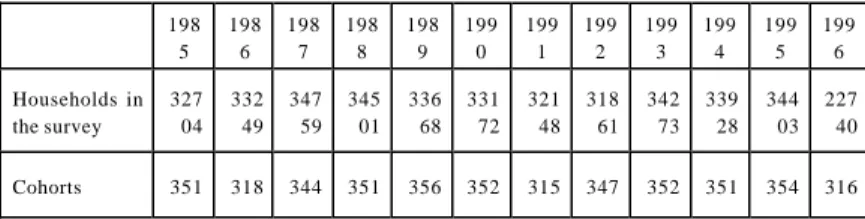
As shown in table 1, the samples used in this paper are composed of more than 32,000 households per year, with the exception of 1996 where only 22,740 households have been interviewed by ISTAT.

6

The methodology of the survey can be briefly described as follows. In a first stage 700 towns and cities are selected and divided into two groups: group 1 includes capitals of provinces and towns with at least 50,000 inhabitants, group 2 includes the rest. A predetermined number of households in towns in group 1 are surveyed each month of the year while towns in group 2 are divided into three further subgroups and each subgroup participates the survey in the first. second or third month of each quarter of the year. Summarizing, each month approximately 320 towns are surveyed: 140 of them belonging to group 1 above and 180 to group 2. In second stage 3000 households per month are randomly selected from the registrar’s offices of the selected towns, thus giving a total of 36,000 households surveyed in the year. The rate of participation in the survey has been approximately estimated around 85%. The initial results are then related to the population by ISTAT.

Table 1 – Number of households and cohorts in the survey

As the household is not re-interviewed every consecutive year, we created a pseudo panel by selecting approximately 350 cohorts of households each year. More specifically, we split the whole sample according to the following categories: date of birth (we group people born in an interval of five years, starting from 1920 to 1972), sex, geographical macro-region and education (up to primary school – middle school - up to secondary school, graduate school). All households having in common the variables listed above have been grouped in a cohort. The individual data are therefore replaced by cohort data7.

Given that our proxy for income innovations will be based on the variability of the net earnings of the head of the household, we limit our sample to those households whose head is recorded as employed in all waves. We further restrict the sample to those households whose head is aged between 25 and 65, and for whom there are valid data on expenditure, occupation, education, and net earnings. These restrictions bring the sample size of our unbalanced pseudo-panel to 4,107 cohort-year observations8. All relevant income and expenditure variables are expressed in 1995 Italian lira9.

7

With this pseudo-panel we have the advantage of observing the same cohort over time while the same was not possible for individuals.

8

Also note that given that our focus is on consumption differences, our empirical analysis will consider only surveys from 1986 to 1985.

9

All variables expressed in value are deflated using the Consumer Price Index.

198 5 198 6 198 7 198 8 198 9 199 0 199 1 199 2 199 3 199 4 199 5 199 6 Households in the survey 327 04 332 49 347 59 345 01 336 68 331 72 321 48 318 61 342 73 339 28 344 03 227 40 Cohorts 351 318 344 351 356 352 315 347 352 351 354 316

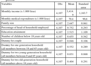
Table 2 presents the summary statistics for the variables of interest, referred to the cohort unit.

Table 2 – Summary statistics at cohort level – Average over the time period

Variables Obs Mean Standard error Monthly income (x 1.000 liras)

4,107 3,414.

9 1,163.7 Monthly medical exp enditure (x 1.000 liras) 4,107 70.4 90,6 Family size 4,107 2.647 0.861 Percentage of head of household employed 4,107 0.752 0.293 Education attainment 4,107 2.515 1.109 Number of children below 18 years old 4,107 0.655 0.562 Dummy for couple 4,107 0.046 0.106 Dummy for one generation household

(all members between 18 and 65 years old) 4,107 0.552 0.289 Dummy for two young-generation household

(all members between 0 and 65 years old) 4,107 0.031 0.068 Dummy for two old-generation household

(all members above 18 years old) 4,107 0.404 0.291

4. - Econometric model and empirical results

In section 2, in order to keep notation simple, the theoretical model has been based on the representative agent. Given that the our data allow for a cohort analysis, in this section we report the empirical model adjusting the functional specification to the cohort unit. As such, we have imposed the only restriction that individual specific effects are common within cohorts.

With the objective of estimating an Euler equation augmented for the presence of two types of uncertainty, we have first obtained a measure for such two sources of uncertainty. We proceed in two steps as follows. As first step, to proxy income and health status innovations, we have obtained residuals from the

following two fixed effect regressions of income and medical expenditures10 aggregated by cohort:

ct c ct ct

Z

Y

=

'

β

+

ε

(7) ct c ct ct M m = 'δ +η (8)

where Z and M are matrices of socio-demographic variables and

c

β and δ the corresponding vector of parameters common to the _c cohort c, to which the agent i belongs to. Each error component, ε and η , is the sum of two separate components:

ε

_ct

=

e

_t

+

e

_ct. The first component of the error term is the time specific effect which accounts for possible business cycle effects, and ect is an

idiosyncratic error term. We take into account the et component

of the error term, by including time dummies in all our specifications.

As second step, we computed the variances of the cohort invariant medical and income shocks from the residuals of the regressions (7) and (8). We then regressed the squared of the predicted error components on its lagged values:

ct t c c t c

ρ

ε

ς

ε

=

2,(−1)

+

2 ,

ˆ

ˆ

(9) ct t c c t c

λ

η

ξ

η

=

2,(−1)

+

2 ,

ˆ

ˆ

(10) 10

Private health expenditure is the sum of expenditures on drugs, physician services and other health care services. In order to get expenditures in real terms, data have been normalized by the relative price indexes.

Finally, we estimated the following Euler equation, where the to set of usual regressors we have added the fitted variances of the two stochastic processes considered in equations (9) and (10):

ct ct ct ct ct ct X C = φ +φ π ε +φ π η +ν ∆ 2 ct 3 2 ct 2 , 1 ' ˆˆ ˆˆ ) ln( (11)

where ∆(Cct) is the consumption rate of growth, Xct’ is a vector of

regressors, π is the scaling factor _ct

2 1 1 2     − − t t c y η σ as in equation (6) and π is made up by three components capturing, respectively, _ct an unobservable cohort-specific time-invariant effect, which we assume to be fixed and captures the unobserved cohort heterogeneity; a time-specific effect that is estimated through a set of time dummy variables, and an idiosyncratic error term.

In the empirical analysis the set of regressors used for equation (7) are income lagged once, head of household’s age and age squared, the number of components in the household, the professional activity of the head of the household and a set of dummy variables related to each cohort group. Similarly, in equation (8) to obtain the predicted component of cohort medical expenditures the set of regressors used are: head of household age, age squared, age cube and the cohort level of medical expenditures lagged once12. Finally, to estimate the augmented Euler equation (11) we have used the following variables as regressors: proportion of heads of the household with the status of “employee” in the cohorts, household size, the absolute change in income (to take into account the possibility of liquidity constraints),

12

We used a fixed effect panel estimate to take into account the specific individual effect in the income and medical expenditure process.

the head of household age and age squared, several socio demographic variables to take into account household heterogeneity and, to test for precautionary saving, medical and income variances and income variance interacted with the proportion of employees in the households.

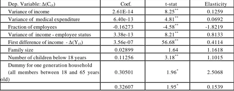
Results from the estimation of equation (11), reported in table 3, show positive and statistically significant values of the parameters referring to medical expenditure and income variance variables, thus indicating the existence of precautionary saving in household behaviour. In terms of elasticities, health expenditure variance has a lower effect (close to half) in determining precautionary saving compared to the income variance, while this last effect is strongly reduced when dealing with heads of household who are classified “employees” compared to “self employed”. At the same time, as the variance of income gets larger, differences between employed and self-employed head of households disappear, as indicated by the positive (meaning that the gap is closed) sign of the parameter of the interaction term between employment status and income variance. No statistical significant result has been obtained interacting employment status with medical expenditure variance. As a further result we observe that level of income has a large positive effect on consumption change, thus proving the existence of liquidity constraints.

Table 3 - Regression results - Observations:3,237 – Cohorts: 396

Dep. Variable: ∆(Cct) Coef. t-stat Elasticity

Variance of income 2.61E-14 8.25** _0.1259

Variance of medical expenditure 6.40e-13 4.81** _0.0692

Fraction of employees -0.16273 -4.58** -1.8219 Variance of income * employee status 3.38e-13 8.21** 0.8133

First difference of income - ∆(Yct) 3.56e-07 56.68** 0.4114

Family size 0.02899 1.64 1.1618 Number of children below 18 years 0.11256 3.18** _1.1015

Dummy for one generation household (all members between 18 and 65 years old)

0.30501 1.96* _2.5068

Dummy for two old-generation household

(all members above 18 years old)

0.13453 0.92 0.8111

Dummy for two young-generation household (all members between 0 and 65 years old) * significant at 5%; ** significant at 1%

In terms of socio-demographic characteristics, family size has the larger impact on precautionary saving: larger households tend to save more (even though the significance of this parameters is only at 10%). The number of children seems also to have a positive effect on postponing household consumption.

An interesting aspect played by the household demographic characteristics is represented by their generational composition. We have classified households in four categories: one generation household, where all member age is between 18 and 65 years (adults); two young-generation households, where at least one member age is between 0 and 18 (child) and at least one member age is between 18 and 65 (adult); two old-generation households, where at least one member age is between 18 and 65 (adult) and at least one member age is above 65 (elderly); and finally three generation household, where at least one member age is between 0 and 18, at least one member age is between 18 and 65 and at least one member age is above 65. The three generation household is our reference household, partly because we assume it is the most sheltered due to the household network that should able to produce (for example, grand parents can assist children and do some housekeeping while parents work). Results show that one generation and two young-generation household have a statistically significant and positive coefficient that proves a higher propensity of these households to have precautionary saving compared to three generation households. A possible explanation for this can be the presence of pensioners in three generation household whose source of income is less volatile than others. As further proof, the two old-generation household (that includes

pensioners) is not statistically significant, thus meaning that there is no difference with the reference household.

5. - Conclusions

In this paper we have explored how saving decisions of Italian households respond to income and health risk. The empirical results show that Italian households appear to use precautionary saving as a device to protect themselves against both health and income risk. Estimates show positive and significant coefficients of the two stochastic processes innovations, with income uncertainty that has a stronger effects compared to health expenditure uncertainty. Households with “self-employed” head of the household are more sensible to income variance compared to “employed” head of household, thus reinforcing the assumption that self employed are more prone to income risk (Skinner, 1988). Liquidity constraints significantly inhibit consumption decisions. Households increase their consumption level only after income realisations, showing a positive coefficient on income changes. Finally, the demographic characteristics and the generational composition of households seem to have an important effect on precautionary saving decisions, with young households that tend to have a higher propensity to save for precautionary reasons.

While the significance of income uncertainty on precautionary saving should not be interpreted as a novel aspect compared to other results in the literature, the role played by the health expenditure variance is instead novel and very interesting. It becomes even more interesting if we consider the presence of a National Health System in Italy that should shelter everybody from unexpected health risk. In fact, recent work on UK consumers from Guariglia and Rossi (2000) have instead proved that health risks do not have effects on precautionary saving of UK household. This might be due to the fact that, in spite of the numerous criticisms surrounding the quality of its services, the NHS is considered after all as a reliable institution in UK. A possible explanation of such results for Italy can ascribed to the

major reorganizations that the NHS has undergone during the ‘90s and that have resulted, among other things, in a larger participation of Italian household to the financing of the health system from one side (increase in co-payment), and to the perception of a global deterioration of the average quality of services provided by NHS, thus shifting households to include in their choice sets private health services providers.

References

Atella, V., Rosati F.C., (2001) ‘Spesa, equità e politiche sanitarie in Italia negli anni ’90: quali insegnamenti per il futuro’, mimeo -- submitted to “Politica Sanitaria”.

Banks, J., Blundell, R., and Brugiavini, A. (1999), ‘Income Uncertainty and Consumption Growth in the UK.’ Institute for Fiscal Studies Discussion Paper.

Carroll C. D., (1996), “Buffer-Stock Saving and the Life Cycle/Permanent Income Hypothesis”, NBER Working Paper No. W5788

Dardanoni, V. (1991), ‘Precautionary Savings under Income Uncertainty: A Cross Sectional Analysis.’ Applied Economics vol. 23, pp.153-160.

Deaton, A. (1992), Understanding Consumption. Oxford: Oxford University Press.

Guariglia, A. (1998), 'Understanding Saving Behaviour In the UK: Evidence from the BHPS.' Institute for Labour Research Discussion Paper No. 9826.

Guariglia, A., Rossi M.C., (2000), 'xxx xxxx xxx' Institute for Labour Research Discussion Paper No. 9826

Guiso L, Jappelli T, Terlizzese D (1992) Earnings Uncertainty and Precautionary Saving. Journal of Monetary Economics 30: 307-337

Kazarosian M (1997) Precautionary Savings- A Panel Study. Review of Economics and Statistics 79 (2): 241-247

Kotlikoff, L., (1986) 'Health Expenditures and Precautionary Savings, NBER working paper n. 2008.

Merrigan, P. and Normandin, M. (1996), ‘Precautionary Saving Motives: An Assessment from UK Time Series of Cross-Sections.’ Economic Journal vol. 106, pp. 1193-1208. Palumbo, M., (1998), “Uncertain Medical Expenditures and

Precautionary Saving. Near the end of the Life Cycle” forthcoming in the Review of Economic Studies

Shea, J. (1995), 'Myopia, Liquidity Constraints, and Aggregate Consumption: A Simple Test.' Journal of Money, Credit, and Banking vol. 27 (3), pp. 798-805.

Starr-McCluer, M. (1996), “Health insurance and Precautionary Savings”, The American Economic Review vol 86 (1), pp.285-295.

Skinner, J., (1988) “Risky income, life cycle consumption, and precautionary saving”, Journal of Monetary Economics, 22, pp.237-255.

Taylor, M. (ed.) (1996), British Household Panel Survey User Manual. Introduction, Technical Reports, and Appendices. Colchester: ESRC Research Center on Micro-Social Change, University of Essex.

Zeldes, S. (1989), “Optimal Consumption with Stochastic Income: Deviations from Certainty Equivalence”, Quarterly Journal of Economics, 104, pp. 275-298.