”TOR VERGATA”
FACOLTA’ DI INGEGNERIA
DOTTORATO DI RICERCA IN
Ingegneria delle Telecomunicazioni e Microelettronica
CICLO DEL CORSO DI DOTTORATO: XII
Peer-to-Peer multimedia
communication
by
Lorenzo Bracciale
Supervisor Coordinator
Peer-to-Peer (P2P) systems have been invented, deployed and researched for more than ten years and went far beyond the simple file sharing applications. In P2P networks, participants organize themselves in an overlay network that abstracts from the topological characteristics of the underlying physical network. Aim of these systems is the distribution of some kind of resources like contents, storage, or CPU cycles. Users, therefore, play an active role so that they can be considered as client and server at the same time, for the particular service that is provided through the P2P paradigm.
The success of Peer-to-Peer systems is given by the clear benefits of this kind of architecture. Among the most important advantages that come for free with the P2P paradigms we have the lack of a single point of failure as well as the cheaper services that can be offered if users contribute to the provisioning of the service.
Nowadays, indeed, P2P traffic represents a big share of the whole Internet traffic. Besides conventional file-sharing P2P applications, recently P2P streaming systems emerge as a new way to distribute multimedia streams among peers. This technol-ogy is made possible by the advances in terms of access bandwidth capacity which connects users to the Internet backbone. Goal of this dissertation thesis is to study these systems, and give contributes in their performance evaluation. The analysis will aim to evaluate the achieved performance of a system and/or the performance bounds that could be achievable.
In fact, even if there are several proposals of different systems, peer-to-peer streaming performance analysis can be considered still in its infancy and there is still a lot of work to do. To this aim, the main contributes of this dissertation thesis are i) the derivation of a theoretical delay bounds for P2P streaming system ii)
simulator, expressly tailored to reproduce the characteristics of the real-world P2P streaming systems, composed by hundred thousands of intermittently connected users.
The dissertation is organized as follows.
In chapter 1 there is a survey of the state of art of p2p streaming systems, including both “structured” systems where connections in the overlay are almost fixed by a strategy, and “unstructured” where connections and partnerships are setted up in a random way.
Chapter 2 focuses on delay bounds in chunk based p2p streaming systems i.e. those systems that choose to split the multimedia content in pieces called chunks whose size is typically bigger than an IP packet. This chapter presents a novel theoretical bound, its asymptotic closed form expression and the demonstration that it is attainable.
Chapter 3 deals with a practical algorithm called O-Streamline based on the the-oretical work presented in Chapter 2. Differently from the thethe-oretical bound that has been derived under the strong hypotheses of the presence of a global and cen-tralized vision of the whole network and of the absence of peer churn, O-Streamline works in a distributed manner but it is designed to achieve a delay that is very close to the theoretical bound.
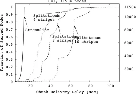
Chapter 4 presents a performance analysis of O-Streamline by means of simula-tions. These simulations are performed using a novel overlay streaming simulator called “OPSS”, expressly tailored to evaluate performance of large scale networks composed by hundred thousands nodes like it happens for real deployed applications. Simulations in a still network and in the case of peer churn show the effectiveness of the O-Streamline algorithm: the achieved delays are very close to the theoretical bound.
Conclusions end the whole dissertation thesis.
In Appendix A, there is a list of my publications related both to P2P multimedia systems, and to other research topics tackled during the Ph.D.
Summary II
1 State of Art of Peer-to-Peer Multimedia Systems 1
1.1 Introduction . . . 1
1.2 Structured P2P Streaming Systems . . . 7
1.2.1 ZigZag . . . 7
1.2.2 SplitStream . . . 8
1.2.3 CoopNet . . . 9
1.2.4 PTree . . . 9
1.3 Unstructured P2P Streaming Systems . . . 10
1.3.1 DONET/COOLStreaming . . . 10
1.3.2 GridMedia . . . 11
1.3.3 PPLive . . . 12
1.3.4 Prime . . . 12
2 Delay Bounds in Chunk Based Peer-to-Peer Streaming Systems 14 2.1 Introduction . . . 14
2.2 Related work . . . 16
2.3 Delay Bound in Chunk Based Peer-to-Peer Streaming Systems . . . . 17
2.3.1 Motivation . . . 18
2.3.1.1 Delay in flow-based systems . . . 18
2.3.1.2 Delay in chunk-based systems . . . 20
2.3.2 Mathematical background: some results on k-step Fibonacci Sums . . . 23 2.3.3 Stream diffusion metric: a delay-related fundamental bound . 27
2.3.3.2 Asymptotic closed form expressions for the bound
on N(t) . . . 32
2.4 Attaining the bound . . . 34
2.4.1 Case k > U and multiple of U: unbalanced multiple trees . . . 36
2.4.2 Case k = U: unbalanced tree . . . 36
2.4.3 The “tree intertwining” problem . . . 39
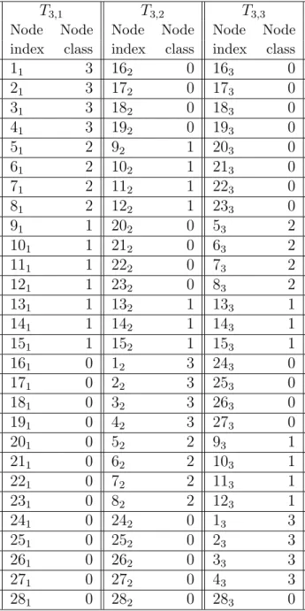
2.4.3.1 Node classes . . . 42
2.4.3.2 Constructive demonstration . . . 45
2.5 Performance Evaluation . . . 47
2.6 Comparison with a literature proposal . . . 47
3 A Theory-Driven Distribution Algorithm for Peer-to-Peer Real Time Streaming 53 3.1 Introduction . . . 53
3.2 O-Streamline: a distributed scheduling algorithm that approximate the delay bounds . . . 54
4 Performance analysis of Peer-to-Peer Streaming Systems 57 4.1 Introduction . . . 57
4.2 State of art of performance evaluation systems and metrics . . . 58
4.3 OPSS: an Overlay Peer-to-peer Streaming Simulator for large-scale networks . . . 62
4.3.1 How does OPSS achieve scalability? . . . 62
4.3.2 Implementation details . . . 64
4.3.3 Performance metrics . . . 65
4.3.4 The evaluated P2P streaming algorithms . . . 68
4.3.4.1 Balanced M-ary tree . . . 69
4.3.4.2 Trivial mesh . . . 74
4.3.5 Simulator performance . . . 78
4.4 O-Streamline performance evaluation . . . 78
4.4.1 Comparison with Streamline, no churn . . . 80
Bibliography 90
State of Art of Peer-to-Peer
Multimedia Systems
1.1
Introduction
Overlays and Peer-to-Peer (P2P) networks, initially developed to share files among different users, have gone a long way beyond that functionality. The first P2P network dates back to 1999, when an 18-year-old college dropout named Shawn Fanning stayed awake 60 hours writing the source code of a program for sharing and swapping music files over the Internet, through a centralized index server. That program was Napster [1], the first wide-used P2P file sharing application. From then on, even if a lawsuit filed by the Recording Industry Association of America (RIAA) forced Napster to shut down the file sharing service of digital music, P2P paradigm usage has continued to grow.
In a Peer to Peer network, users (“peers”) plays the role of client and server, being both producer and consumer of the service the network offers. In this way, the burden of providing a specific service (e.g. buying servers, bandwidth capacity, network devices) is shared among users and the content provider, making cheaper and easier to setup such kind of network.
Moreover this kind of networks offer implicitly an highly desirable fault-tolerance, self-organization and massive scalability properties.
service. We can distinguish between ”pure” peer-to-peer systems in which the entire network consists solely of equipotent peers. There is only one routing layer, as there are no preferred nodes with any special infrastructure function. Otherwise we can have ”Hybrid” peer-to-peer systems that rely on such infrastructure nodes, often called supernodes. Another characteristic of a peer to peer network is the structure. We have structured peer-to-peer networks where connections in the overlay are al-most fixed by a strategy. On the contrary, in unstructured peer-to-peer networks often connections and partnerships are setted up in a random way
All these strategies has their pro and cons. Typically, structured P2P networks ob-tain better performance at steady-state, but when the amount of peers that leave or join the network increases (peer churn) they could suffer of instability or they should need and high volume of traffic to keep the network consistent to the given structure.
P2P overlays have been deployed in many different application areas.
When users share CPU cycles, they make distributed computing possible. The SETI@home project [2] uses for example a virtual supercomputer composed of large numbers of Internet-connected computers, with the goal of analyzing radio tele-scope signals from space and detecting intelligent life outside Earth. The Compute Against Cancer [3] program takes advantage from Frontier, a distributed computing platform by Parabon Computation, to understand and reduce the side effects of chemotherapy, study the structure and behaviour of cancer cells and create better ways to screen new cancer drugs.
P2P systems can be used also to share disk storage allows for creating distributed file systems. The authors of [4] propose Cooperative File System (CFS), a peer-to-peer completely decentralized read-only storage system that provides efficiency, robustness and load-balance of file storage and retrieval.
Skype[5] is probably the best examples of how P2P technology may be ex-ploited in the consumer market. Skype is a software application that allows users to make voice calls over the Internet that today has more than 521 millions of users (20,365,656 concurrent Skype users were online November 9, 2009) with a revenue
of more than 185 millions of USD.
P2P file sharing networks are perhaps the most popular P2P application. In this case peers share their own files and, once contents of interest are localized in the network, direct connections are established between peer requesting content and peer storing it to make file transfer possible.
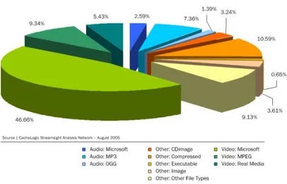
Figure 1.1. Peer to Peer traffic represents a big share of the whole Internet traffic
According to measurement studies in Figure 1.1, P2P file sharing traffic dom-inates Internet traffic. Moreover Figure 1.2 pointed also out a user demand shift-ing from music files towards video files. BitTorrent [6][7] is undoubtedly the most widespread P2P file sharing application. Gnutella [8][9], KazaA [10][11][12], eDon-key [13] were others example of wide used P2P software for file sharing, at least in the past. All of them have several accidents with law and ended with their closure, while the open source counterpart of eDonkey, eMule, keeps instead on existing by eliminating the presence of any central server that can get in trouble with authorities for the copyright issues. Nowadays eMule, like other P2P programs, uses a com-pletely distributed searching system based on a structured organization on peers called Distributed Hash Table (DHT) .
DHTs assign uniform random NodeIDs from a large space of identifiers to the overlay peers. Data objects or values are distinguished with an unique identifiers called keys, chosen from the same identifier space. Keys are mapped by the overlay network protocol to a unique live peer in the overlay network so that there is at least one peer in the system that knows where data is (the node with ID nearer to the key). Each peer maintains a small routing table consisting of its neighboring peers’ NodeIDs and IP addresses. Lookup queries or messages are forwarded across overlay paths to peers in a progressive manner. In other words, queries are always routed to the peer with the NodeID that is closest to the key in the identifier space. Naturally, different DHT-based systems will have different organization schemes for the data objects, key space and routing strategies. However, regardless of the organization schemes, DHT-based systems may guarantee that any data object can be located in a number of hops that grows on average sub-linearly (usually logarithmically) with the number N of network nodes. Moreover, the underlying network path between two peers can be significantly different from the path on the DHT-based overlay network. Therefore, the lookup latency in DHT-based P2P overlay networks can be quite high and could adversely affect the performance of the applications running over it. Dif-ferently from unstructured ones, structured P2P networks can efficiently locate rare items since key-based routing is scalable. They however incur significantly higher overheads than unstructured P2P networks for popular content because all keys are distributed in the same way, regardless from the popularity of the data they refer to.
Recently, the speedup of the users available access bandwidth paved the way to P2P overlay networks aimed to provide video streaming to all the participant. Among the motivation of the success of such kind of applications, there were the explosive growth of multimedia services and applications and the the several diffi-culties in which incurs the deployment of IP multicast. Even if IP multicast has originally been introduced with the purpose of offering point-to-multipoint content distribution services, many deployment issues have still to be solved. As argued in [14], IP multicast calls for multicast-capable routers able to maintain per group state information, which seriously limit its scalability when groups grow up. Sec-ond, IP multicast is a best effort service, and providing higher level features such as reliability, congestion control, flow control, and security has been shown to be more difficult than in the unicast case. Finally, IP multicast requires changes at the infrastructure level, and this slows down the deployment pace.
Due to this, more and more researchers are investigating application level mul-ticast as solution to stream multimedia audio and video content from a source to a large number of end users. This approach consists of end hosts, which according to peer-to-peer (P2P) paradigm auto-organize themselves in an overlay network out of unicast tunnels across participating overlay nodes. Relaying data among overlay nodes allows then the multicast service.
Overlay multicast distribution trees represent the most natural way of extending IP level multicast to application level. To name a few, NICE [15], ZIGZAG [16], CoopNet [17], SplitStream [18] are tree-based P2P streaming systems. However, while tree-based topologies are well suited to dedicated IP multicast routers, they could suffer from re-configurability problems in presence of high churn rate of P2P nodes. In reason of this, overlay mesh-based and unstructured topologies have also been proposed. CoolStreaming/DONet [19] and GridMedia [20] offer examples of the latter approach.
The main disadvantage to using a P2P approach is that it is hard to provide de-livery guarantees because peer failures, departures, and disconnections are common.
Goal of all the P2P multimedia streaming systems is to provide data to all the participant of the overlay, with some time constraint given by the streaming nature of the service: usually data must arrive to the user as soon as possible, but no later than a deadline (sometimes called “playback deadline” ) that is when this data must be used by the user streaming application to play the part of the video data contains.
To achieve this goal, a plethora of very different distribution algorithms have been proposed up to now. These algorithms make specific and different assumptions and choices about the main aspects of a P2P real time streaming system, such as overlay topology, scheduling process and upload strategy.
Sometimes the multimedia flow is divided in pieces called “chunks”, and goal of the network is to organize peer nodes in an overlay distribution network to relay chunks. Before summarize the different approaches known in literature and in “real-world” applications, I want to classify the different kind of choices operated by all these approaches.
First categorization regards the overlay topology. It is possible to distinguish among:
• tree-based solutions, such as NICE [15] and ZIGZAG [16], where nodes are organized in a tree and content is recursively spread from the parent node (the streaming source) to its child nodes until all peers are reached;
• mesh-based solutions, such as CoolStreaming [19], Gridmedia [20] or PRIME [21], where each node randomly establishes overlay connections with other nodes and sends a received chunk only to neighbors still missing that chunk, in such a way that each chunk is streamed on a different tree;
• forest-based solutions, such as CoopNet [17] or SplitStream [18], where chunks and nodes are logically organized in a finite set of groups and distribution trees, in such a way that each distribution tree includes all nodes and is used to distribute a single group of chunks. Nodes are interior nodes only in one tree and leaf nodes in all the remaining trees. The idea is to exploit the upload capacity that leaf nodes do not use in separate distribution trees, thus
increasing the overall transmission capacity of the overlay network. As regards the scheduling process, it is possible to distinguish among:
• push-based algorithms, such as [15] and [16], where supplier nodes decide which chunks will be served to which neighbors;
• pull-based algorithms, such as [19] or [21], where scheduling decisions are taken at receivers and a chunk is transmitted only if a receiver requests that chunk; • hybrid push-pull algorithms, like [20], where chunks are requested in pull mode
at start up and relayed in push mode in the immediate following phase. Moreover, different local scheduling policies have been proposed: for instance, giving priority to the chunks with more stringent playback deadline [19], to the rarest chunks [22], to the neighbors with the highest upload/download capacity [19][23]. As regards the upload strategy, when the same chunk has to be uploaded to more than one child node, it can be transmitted “in series”, e.g. starting the transmission towards a second child node after completion of the chunk upload to the first child, or “in parallel”, i.e. sending the same chunk to more than one child node at the same time.
In what follows I will survey the most relevant peer to peer streaming systems.
1.2
Structured P2P Streaming Systems
1.2.1
ZigZag
ZIGZAG [16] deals with the problem of one source towards multiple destinations with consideration of network condition. The goals are to minimize the E2E delay, to manage user dynamicity and to keep the overhead traffic as small as possible to achieve scalability.
To realize this objective, ZIGZAG organizes receivers into a hierarchy of bounded-size clusters and builds the multicast tree based on that. The connectivity of this tree is enforced by a set of rules, which guarantees that the tree always has a height O( logkN ) and a node degree O( k2 ), where N is the number of receivers and k a
constant. The proposed approach helps in reducing the number of processing hops processing to avoid the network bottleneck. At the same time ZIGZAG handles the effects of network dynamics requiring a constant amortized control overhead. Peers are organized in a multi-layer hierarchy of clusters. The cluster size is upper bounded by 3k so that if it has to split because of oversize, the two new cluster are big enough to do not risk to as peers leave.
1.2.2
SplitStream
In SplitStream the stream is stripped into k stripes to be distributed across a forest of overlay multicast trees. The construction of the overlay multicast trees is based on Scribe [24]. Scribe is an application-level group communication system built on top of Pastry [25], which is a DHT-based self-organizing, structured, P2P overlay network. The key idea is the following: each multicast group is associated with a pseudo-random Pastry key, and the corresponding multicast overlay tree is formed by the union of the Pastry routes from each group member to the root node1 for that group Pastry key.
In more detail, SplitStream uses a separate Scribe multicast tree for each of the k stripes. A fundamental property of the SplitStream overlay trees is that they are interior-node-disjoint trees. In other words, SplitStream nodes are organized into overlay trees in such a way that each node is interior node in at most one tree and leaf node in the remaining trees. To realize these trees, it uses the Pastry mechanism to forward message: each Pastry node indeed forward each message to node whose nodeId share a progressively longer prefix with the message’s key. Since each Scribe multicast tree is formed by the union of the routes from all members to the groupId, nodeIds of all the interior nodes share some number of digits with the tree groupId. Therefore, by choosing groupId that differs in the most significant digit, we are obtaining trees with disjoined sets of interior nodes. The number of stripes determine the incoming bandwidth usage, each node is at least expected to forward k. If a SplitStream node has exceeded its outgoing capacity and receives a
1The root node for a Pastry key is the node with the identifier that is numerically closest to
request, one child is dropped according to given criteria. This child node first tries to attach to one of its former siblings. Otherwise, it searches the “Spare capacity group” for a node that is able to provide to it the requested stripe.
1.2.3
CoopNet
Coopnet is an application level multicast system developed to overcome the so called “flash crowd” scenario, where an unexpected increase of demand for a popular con-tent, causes an unsustainable bandwidth request at a server (as happened to the MSNBC streaming server on Sep 11, 2001).
In this sense, a Peer-to-Peer based approach could solve this problem, in reason of its self-scaling propriety, so that the system scale well with the users grows without requiring any new infrastructure. On the other hand, peer churn can make the ser-vice highly unreliable. CoopNet aims to become resilient to the transience of peers by utilizing redundancy in network paths and redundancy in data. To achieve this goal, the CoopNet protocol anchors itself at a central server that manages multiple distribution trees of peers. The server also encodes data using Multiple Descrip-tion Coding (MDC) to provide redundancy in data and the encoded data is then distributed to clients using the different distribution trees . MDC is constructed so that any subset allows the client to reconstruct the video so that if a node fails, the user might still get video.
CoopNet protocol is quite simple because it relies on a centralized server. Nodes inform the server when they join and leave they indicate available bandwidth and the delay coordinates so basically the server maintains the trees and nodes could monitor loss rate on each tree and seek new parent(s) when it gets too high.
1.2.4
PTree
The inspiration for PTree was taken by Splitstream. The distribution architecture of PTree (formalized in [65]) organizes peers in k overlay trees, in such a way that: i) each tree includes all peers and ii) each peer is interior node in at most one tree and leaf node in all the remaining trees. The root nodes of the k trees are children of
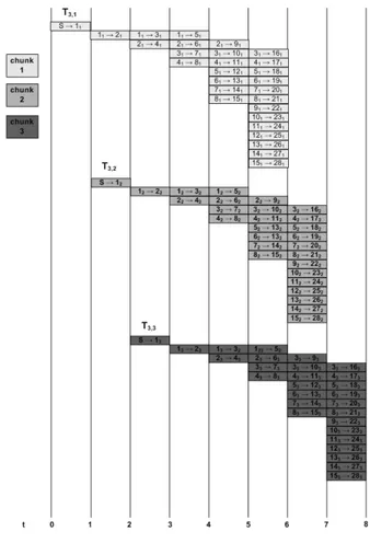
Figure 1.3. PTree distribution architecture; 15 nodes network.
the source. The multimedia flow is divided into chunks and the source always serves k different chunks to its children by means of parallel transmissions; each interior node does the same and serves each received chunk to its k children by means of parallel transmissions. Figure 1.3 illustrates such distribution architecture for the case k = 2 and a network of 15 nodes. In this figure the source is denoted with an “S” and nodes are progressively indexed starting from 1. Note that the distribution patterns in figure 1.3 actually relate to the first two chunks and repeat themselves with period k = 2. To achieve an homogeneous node operation it has been assumed that the source starts to transmit the first 2 chunks only when both are available. This happens at time unit t = 1, i.e. after the time required to transmit a chunk at the rate B. The source ends transmitting the first 2 chunks at time unit t = 3. Since at this time two new chunks will be available, it starts transmitting these 2 chunks, and so on.
1.3
Unstructured P2P Streaming Systems
1.3.1
DONET/COOLStreaming
CoolStreaming/DONet [19] is a live media streaming system which constructs a random overlay mesh to distribute the stream segments between the participating overlay nodes. Chunk availability in the node buffer is represented by bit vector called Buffer Map (BM), where a bit 1 and 0 indicate that a segment is respectively
available or unavailable. Each node learns about chunk availability by periodically exchanging its BM with the BMs of its partners, which are the neighbors in the overlay mesh. DONet is built on a pull approach, i.e. scheduling decisions are taken at receivers and chunk transmissions start only if a receiver requests that chunk from a supplier neighbor. Specifically, the proposed heuristic scheduling algorithm gives priority to the chunks with more stringent playback deadline and to supplier neighbors with the highest bandwidth. So the algorithm calculates the number of potential suppliers for each segment and, starting from the segments with only one potential supplier, it selects the supplier with the highest bandwidth and enough available time in case of multiple suppliers.
1.3.2
GridMedia
GridMedia [20] is an unstructured P2P live media streaming system which tries to overcome the limitation of the DONet pull approach to achieve a minor delay. It is based on a push-pull approach that consists in requesting stream packets in pull mode at start up and having nodes relaying stream packets in push mode (e.g. without explicit request) in the immediate following phase.
The same authors as [20] focus in [22] on the optimal streaming scheduling problem in data-driven overlay networks. The optimal streaming scheduling problem aims at addressing how each node optimally decides from which neighbor to request which block, and how it allocates its limited outbound bandwidth to every neighbor, in order to maximize the throughput. This scheduling problem is formulated as a classical min-cost network flow problem and two resolution strategies are considered. The first one is a global optimal solution which assumes a centralized knowledge of all network state, the second one is an heuristic algorithm which is fully distributed and calls for only local information exchange.
Gridmedia was adopted by CCTV to broadcast the CCTV Spring Festival Gala 2005 through Internet and attracted more than 500.000 users all over the world during that night, with the maximum amount of concurrent users reaches as high as 15.239.
1.3.3
PPLive
PPLive [26] is by far the most popular video streaming client. Both protocol and application is proprietary but thanks to some reverse engineering work such [27] we are able to better understand its behaviour. PPlive aims to construct a mesh but it relies also on the help of some servers/supernodes. It exhibits a very aggressive be-haviour both in contacting new peers than in using node bandwidth to forward video content. Because of the nature of the streaming whose chunks have hard deadlines, PPLive introduces some buffers (and therefore some delays) to have enough time to react to node failures and to smooth out the jitter. In particular we can distinguish between two buffers: one is managed by PPLive, the second by the media player. A downside of such an architecture is the long startup delay. In PPLive we can consider two types of delay: i) the interval between channel selection and media display ( 10 to 15 seconds), and; ii) the playback time, required for fluent playback in spite of jitter ( 10 to 15 more seconds). The time lag between nodes may range up to about one minute.
On January 28, 2006 PPLive delivered a very popular TV program in China, host-ing over 200K users, at data rates to users between 400 and 800Kbps, reachhost-ing an aggregate bit-rate of 100Gbps.
1.3.4
Prime
In PRIME [21] participating peers form a randomly connected and directed mesh, where all connections are congestion controlled. The incoming and outgoing degrees of individual peers are determined by maximizing the utilization of the incoming and outgoing access link bandwidth. The content is encoded with Multiple Description Coding (MDC) which enables each peer to maximize the delivered quality by pulling a proper number of descriptions. With regard to the content delivery mechanism, PRIME combines push advertisements by parents with pull requests by child peers. The packet scheduling mechanism at child peers selects the packets to be requested according to a global pattern of content delivery that minimizes the probability of content bottleneck among peers. Such pattern consists of the diffusion and the swarming phases. The diffusion phase relates to the new stream segments that have been advertised by parents during the last scheduling event. The swarming phase
relates to the packets that have already been received and are within the playout buffer. Specifically, for each received packet within the playout buffer, the scheduling algorithm determines the number of missing descriptions according to the target delivered quality and assigns each identified packet to a parent that can provide it. The stream source is instead required to implement optimized mechanisms to minimize the potential overlap among the packets delivered to different children. Performance of PRIME has been evaluated via packet-level ns [47] simulations. The number of simulated nodes ranges from 100 to 500. Access links are considered symmetrical and are assigned a bandwidth of 700 Kbps and/or 1.5 Mbps respectively in the heterogeneous and homogeneous scenario. The stream has 10 descriptions and each description has bit rate of 160 Kbps.Performance metrics related to delivered quality, content bottleneck occurrence during the diffusion and swarming phase, bandwidth bottleneck, playout buffer capacity and average path length of delivered packets are presented.
Delay Bounds in Chunk Based
Peer-to-Peer Streaming Systems
2.1
Introduction
In this chapter we focus on chunk-based systems, where, similarly to most file-sharing P2P applications, the streaming content is segmented into smaller pieces of infor-mation called chunks. Chunks are elementary data units handled by the nodes composing the network in a store-and-forward fashion. A relaying node can start distributing a chunk only when it has completed its reception from another node. While the solutions based on multicast overlay trees usually organize the informa-tion in form of small IP packets to be sequentially delivered across the trees and can not be regarded as chunk-based, some data-driven solutions, like the ones proposed in [19] [21] [56], may be regarded as chunk-based. A characterizing feature of the chunk-based approach is that, in order to reduce the per-chunk signalling burden, the chunk size is typically kept to a fairly large value, greater than the typical packet size.
In this chapter we raise some very basic and foundational questions on chunk-based systems: what are the theoretical performance limits, with specific attention to delay, that any chunk-based peer-to-peer streaming system is bounded to? Which fundamental laws describe how performances depend on network parameters such as the available bandwidth or system parameters such as the number of nodes a
peer may at most connect to? And which are the system topologies and operations which would allow to approach such bounds?
Surprisingly enough, according to the best of our knowledge and our literature survey, these questions have never been directly posed before, and answered, for chunk-based systems (the only references somewhat related to these issues are [57] for the file sharing case, and [58] for the streaming case). The aim of this chapter is to answer these questions. The answer is completely different from the case of systems where the streaming information, optionally organized in sub-streams, is continuously delivered across overlay paths (for a theoretical investigation of such class of approaches refer to [59] and references therein contained). As we will show, in our scenario the time needed for a chunk to be forwarded across a node significantly affects delay performance.
In more detail, we focus on the ability to reach the greatest possible number of nodes in a given time interval (this will be later on formally defined as “stream diffusion metric”) or equivalently the ability to reach a given number of nodes in the smallest possible time interval (i.e. absolute delay). We derive analytic expressions for the maximum asymptotic stream diffusion metric in an homogeneous network composed of stable nodes whose upload bandwidth is the same (for simplicity, mul-tiple of the streaming rate).
With reference to such homogeneous and ideal scenario, we show how this bound relates to two fundamental parameters: the upload bandwidth available at each node, and the number of neighbors a node may deliver chunks to. In addition, we show that the serialization of chunk transmissions and the organization of peer nodes into multiple overlay unbalanced trees allow to achieve the proposed bound. This suggests that the design of real-world applications could be driven by two simple basic principles: i) the serialization of chunk transmissions, and ii) the organization of chunks in different groups so that chunks in different groups are spread according to different paths.
This chapter is organized as follows. Section 2.2 surveys the state of the art related to delay in p2p streaming systems. Section 2.3 shows a new discovered bound for streaming. Section 2.4 shows that the bound is also attainable. In section 2.5 there is a performance evaluation of the optimal scheduling solution respect to other kind of simple scheduling strategies. Finally in the section 2.6 there is
a comparison with other literature proposed systems. The work presented in this chapter is realized in team work with professors Giuseppe Bianchi, Nicola Blefari Melazzi, Stefano Salsano and colleagues Francesca Lo Piccolo and Dario Luzzi.
2.2
Related work
The literature abounds of papers proposing practical and working distribution al-gorithms for P2P streaming systems; however very few theoretical works on their performance evaluation have been published up to now. As a matter of fact, due to the lack of basic theoretical results and bounds, common sense and intuitions and heuristics have driven the design of P2P algorithms so far.
The few available theoretical works mostly focus on the flow-based systems, as they have been defined in subsection 2.3.1.1. In such case, a fluidic approach is typically used to evaluate performance and the bandwidth available on each link plays a limited role with respect to the delay performance, which ultimately depend on the delay characterizing a path between the source node and a generic end-peer. This is the case in [59] and [60]. Moreover, there are also other studies that address the issue of how to maximize throughput by using various techniques, such as network coding [61] or pull-based streaming protocol [62].
This work differs from the previously cited ones mainly because it focuses on chunk-based systems, for which discrete-time approaches are most suitable than fluidic approaches. Surprisingly enough, according to the best of our knowledge and our literature survey, there is only one work [58] where chunk-based systems are theoretically analyzed. In more detail, the author of [58] derives a minimum delay bound for P2P video streaming systems, and proposes the so called snow-ball streaming algorithm to achieve such bound. Like the theoretical bound presented in this chapter, the bound in [58], that is expressed in terms of delay in place of stream diffusion metric, can be achieved only in case of serial chunk transmissions and it is equivalent to the one that we found as a particular case when k → ∞. However, the assumptions under which such bound has been derived in [58] are completely different. In fact, with reference to a network composed of N = 2l nodes excluding the source node, the proposed snow-ball algorithm for chunk dissemination requires
that i) the source node serves each one of the N = 2l network nodes with different chunks, ii) nodes other than the source serve l different neighbors. In other words, the resulting overlay topology is such that i) the source node is connected to all the N network nodes, ii) nodes other than the source have log2N overlay neighbors. Due to this, our approach may be definitely regarded as significantly different from the one in [58]. Differently from [58], we indeed consider the case of limited overlay connectivity among nodes and we show that organizing nodes in a forest-based topology allows to achieve performance very close to the ones of the snow-ball case.
2.3
Delay Bound in Chunk Based Peer-to-Peer
Streaming Systems
This section addresses the following foundational question: what is the maximum theoretical delay performance achievable by an overlay peer-to-peer streaming sys-tem where the streamed content is subdivided into chunks? When posed for chunk-based systems, and as a consequence of the store-and-forward way in which chunks are delivered across the network, this question has a fundamentally different an-swer with respect to the case of systems where the streamed content is distributed through one or more flows (sub-streams). To circumvent the complexity emerging when directly dealing with delay, we express performance in term of a convenient metric, called “stream diffusion metric” defined in section 2.3.3. We show that it is directly related to the end-to-end minimum delay achievable in a P2P streaming network. In a homogeneous scenario, we derive a performance bound for such met-ric, and we show how this bound relates to two fundamental parameters: the upload bandwidth available at each node, and the number of neighbors a node may deliver chunks to. In this bound, presented in 2.3.3, k-step Fibonacci sequences do emerge, and appear to set the fundamental laws that characterize the optimal operation of chunk-based systems. The contribute in the theory of n-step Fibonacci sums for which a prior reference result was missing is presented in section 2.3.2.
2.3.1
Motivation
Goal of this section is to clarify why P2P chunk-based streaming systems have sig-nificantly different performance issues with respect to streaming systems, where the information content continuously flows across one or more overlay paths or trees. Unless ambiguity occurs, such systems will be referred to as, with slight abuse of name, flow-based systems. More precisely, we will show that i) theoretical bounds de-rived for the flow-based case may not be representative for chunk-based systems, and new, fundamentally different, bounds are needed, ii) the methodological approaches which are applicable in the two cases are completely diverse, and fluidic approaches may be replaced with inherently discrete-time approaches where, as shown later on, k-step Fibonacci series and sums enter into play.
2.3.1.1 Delay in flow-based systems
We recall that “flow-based” system denotes a stream distribution approach where the streaming information, possibly organized in multiple sub-streams, is delivered with continuity across one or more overlay network paths. Clearly, in the real IP world, continuous delivery is an abstraction, as the streaming information will be delivered in the form of IP packets. However, the small size of IP packets yields marginal transmission times at each node. As such, the remaining components that cause delay over an overlay link (propagation and path delay because of queueing in the underlying network path) may be considered predominant. We can conclude that the delay performances of flow-based systems ultimately depend on the de-lay characterizing a path between the source node and a generic end-peer. More specifically, if we associate a delay figure to each overlay link, then the source to destination delay depends on the sum of the link delays: the transmission times needed by the flow to “cross” a node may be neglected, or, more precisely, they play a role only because the ‘crossed” nodes compose the vertices of the overlay links, whose delays dominate the overall delay performance.
As a consequence, the delay performance optimization becomes a minimum path cost problem, as such addressed with relevant analytical techniques. If we further assume that the network links are homogeneous (i.e. characterized by the same delay), then the problem of finding a delay performance bound is equivalent to
Figure 2.1. Tree depth optimization in flow-based systems. A tree depth equal to 2 can be achieved by i) splitting the stream in a number of sub-streams equal to the number of network nodes N, ii) delivering each sub-stream to a different node, and iii) letting each node i replicate and deliver the i-th sub-stream to the
remaining N − 1 nodes.
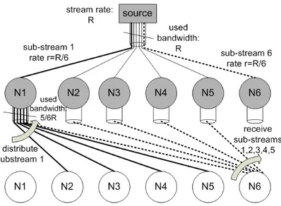
finding what is the minimum depth of the tree (or multiple trees) across which the stream is distributed. This problem has been thoroughly addressed in [59], under the general assumption that a stream may be subdivided into sub-streams (delivered across different paths), and that each node may upload information to a given maximum number of children. For instance, if we assume no restriction on the number of children a node may upload to, then it is proven in [59] that a tree depth equal to two is always sufficient. This is indeed immediate to understand and visualize in the special case of all links with a “sufficient” amount of available upload bandwidth - see figure 2.1 for a constructive example1.
At this stage, it should be clear that, in the context of flow-based systems, as long as some feasibility conditions are met (see e.g. [60]), the bandwidth available on each link plays a limited role with respect to the delay performance achievable. This is clearly seen by looking again at figure 2.1: if for instance we double the
1In this example, the amount of available upload bandwidth is “sufficient” in the sense that the
source node has a bandwidth at least equal to the stream bit rate R, while each peer node has a bandwidth at least equal to (N − 1) · R/N, being N the number of peer nodes composing the overlay. As shown in [59] the same result holds under significantly less restrictive assumptions on the available bandwidth.
bandwidth available on each link, the delay performances do not change (at least until the source is provided with a large enough amount of bandwidth to serve all peers in a single hop).
2.3.1.2 Delay in chunk-based systems
Chunk-based systems have a key difference with respect to flow-based systems: the streaming information is organized into chunks whose size is significantly greater than IP packets. Since a peer must complete the reception of a chunk before for-warding it to other nodes (i.e. chunks are delivered in a store-and-forward fash-ion), the obvious consequence is that delay performance are mostly affected by the chunk transmission time. Thus, in terms of delay performance, the behaviour of chunk-based systems is opposite to the one of flow-based systems. Not only chunk transmission times cannot be neglected anymore with respect to link-level delays (propagation and underlying network queueing), but also we can safely assume that in most scenarios any other delay component at the link-level has negligible impact when compared with the chunk transmission times. This consideration can be re-stated as: the delay performances of chunk-based systems do not depend on the sum of the delays experienced while travelling over an overlay link, but depend on the sum of the delays experienced while crossing a node.
From a superficial analysis, one might argue that the overall delay optimization problem does not change. In fact, the transmission delay of a chunk at a given node could be attributed to the overlay link over which the chunk is being transmitted, and, also in this case, the optimization could be stated as a minimum path cost problem.
However, a closer look reveals that this is not at all the case. The reasons are manifold and can be illustrated with the help of figure 2.2. In this figure, and consistently throughout the chapter, we rely on the following notation. C is the chunk size (in bit); Rbps is the streaming constant bit rate (in bps). T = C/Rbps is the chunk “inter-arrival” time at the source, being such arrival process a direct consequence of the segmentation into chunks done at the source: a new chunk will be available for delivery only when C information bits, generated at rate Rbps, are accumulated (see top of figure 2.2). Ubps is the available upload bandwidth, assumed
to be the same for all network nodes, including the source (homogeneous bandwidth conditions). U = Ubps/Rbps is the normalized upload bandwidth of each node with respect to the streaming bit rate. For simplicity, we consider the case of U integer greater or equal than 1, i.e. Ubps being either equal or a multiple of Rbps. The minimum transmission time for a chunk is equal to T∗ = C/U
bps = T /U; this is true only if the whole upload bandwidth Ubps is used to transmit a single chunk to a single node. Moreover, we rely on the common simplifying assumption, in overlay P2P systems, that the only bandwidth bottleneck is the uplink bandwidth of the access link that connects the peer to the underlying network (the downlink bandwidth is considered sufficiently large not to be a bottleneck - this is common in practice, due to the large deployment of asymmetric access links - e.g., ADSL).
The first reason why the overall delay optimization problem can not be stated as a minimum path cost problem in the case of chunk-based systems is the sharing of the available upload bandwidth Ubpsacross multiple overlay links. As a consequence, i) it is not possible to a priori associate a constant delay cost to overlay links originating from a given node, ii) the delay experienced while transmitting a chunk depends on the fraction of the bandwidth that the node is dedicating to such transmission. For instance, figure 2.2 shows that the source node is transmitting a given chunk in parallel to two nodes; as such, the transmission delay is C/(Ubps/2). If the source were transmitting the chunk only to node 1, this delay would be halved.
The second reason is that the transmission time may not be the only component of the overall chunk delivery delay. This is highlighted for the case of node N1. After receiving chunk 1, node N1 adopts the strategy of serializing the delivery of chunk 1 to nodes N4 and N5. On the one side, in both cases the chunk will be transmitted in the same time, namely C/Ubps; this is the minimum transmission time for a chunk, as all the available bandwidth is always dedicated to a single transmission. On the other side, the time elapsing between the instant at which the chunk is available at node N1 and the instant at which the chunk is received by node N5 is greater than the transmission time, as it includes also the time spent by node N1 while transmitting the chunk to node N4.
The third and final aspect which characterizes chunk-based systems in a stream-ing context is that there is a tight constraint which relates the number of peer nodes that can be simultaneously served and the available upload bandwidth. If
Figure 2.2. Delay components and constraints in chunk-based systems.
we look back flow-based systems in figure 2.1, we see that only practical imple-mentation issues may impede the source node to arbitrarily subdivide the stream into sub-streams, and the tree depth may be indeed trivially optimized by using as many sub-streams as the number of nodes in the network. On the contrary, in chunk-based systems, the number of nodes that can be served is no more a “free” parameter, but it is tightly constrained by the stream rate and the available upload bandwidth. This fact can be readily understood by looking at the source node in the example illustrated in figure 2.2. Due to their granularity, new chunks are available for delivery at the source node every T = C/Rbps seconds. Hence, in order to keep the distribution of chunks balanced (i.e., to avoid introducing delays with respect to the time instant at which chunks are available at source and to privilege specific chunks by giving them extra distribution time), the source node must complete the delivery of every chunk before the next new chunk is available for the delivery (i.e. within T seconds). This implies that the source node cannot deliver a single chunk to more than U nodes, being U = Ubps/Rbpsthe ratio between the upload bandwidth
and the streaming rate2.
2.3.2
Mathematical background: some results on k-step
Fi-bonacci Sums
Before stating the bound, we need to provide some preliminary notation and the mathematical background.
Let Fk(i) be the k-step Fibonacci sequence defined as follows:
Fk(i) = 0 if i≤ 0 1 if i = 1 %k j=1Fk(i− j) if i > 1 (2.1)
Let Sk(n) be a new sequence defined as the sum of the first n non-null terms of the k-step Fibonacci sequence, i.e.,
Sk(n) = & 0 if n≤ 0 %n i=1Fk(i) if n > 0 (2.2) While k-step Fibonacci series have been extensively investigated in related lit-erature, to the best of our knowledge, very few results are available on the sum of k-step Fibonacci series. Since these sums play a fundamental role in our analysis, we derive some new key results concerning them.
Lemma 1 Recursive expression for k-step Fibonacci Sums. Let Sk(n), with n≥ 1, be the sum of the first n terms of a k-step Fibonacci sequence as defined in (2.1). Then, Sk(n) may be recursively computed as:
Sk(n) = 1 + k '
i=1
Sk(n−i) ∀n ≥ 1 (2.3)
The proof is based on the mathematical induction. Condition (2.3) is immediately verified for n = 1. Hence, let us assume that condition (2.3) holds for all indices up
2A similar conclusion can be drawn for other nodes as well. Moreover, we remark that this
to n. By applying such condition to Sk(n) and by using the k-step Fibonacci series definition (2.1), it is straightforward to prove that (2.3) holds also for n + 1:
Sk(n + 1) = Sk(n) + Fk(n + 1) = = 1 + k ' i=1 Sk(n−i) + k ' i=1 Fk(n+1−i) = = 1 + k ' i=1 [Sk(n−i) + Fk(n−i+1)] = 1 + k ' i=1 Sk(n+1−i) (2.4)
Lemma 2 Relation between k-step Fibonacci Sums and k-step Fibonacci Series. The following general relation holds
Sk(n) = k ' i=1 (i+1−k)Fk(n+i) k− 1 − 1 k− 1 (2.5)
We also observe that the well known result S2(n) = F2(n + 2)−1, relative to the sum of traditional Fibonacci series (i.e., k = 2), is a special case of equation (2.5) (achievable for k = 2).
The proof requires some algebraic elaboration. We start by reformulating the linear recurrence (2.1) as the following difference equation:
Fk(i) + k−1 ' j=1
Fk(i + j)− Fk(i + k) = 0 ∀i ≥ 1 (2.6)
Since this equality holds for any i≥ 1, it holds also for the sum n ' i=1 & Fk(i) + k−1 ' j=1 Fk(i + j)− Fk(i + k) ( = 0 ∀n ≥ 1 (2.7)
performed on the left-hand member: Sk(n) + k−1 ' j=1 n+j ' i=1+j Fk(i)− n+k ' i=1+k Fk(i) = = Sk(n) + k−1 ' j=1 ) n ' i=1 Fk(i) + n+j ' i=n+1 Fk(i)− j ' i=1 Fk(i) * + − n ' i=1 Fk(i)− n+k ' i=n+1 Fk(i) + k ' i=1 Fk(i) = = (k− 1) Sk(n) + k−1 ' i=1 (k− i)Fk(n + i)− k ' i=1 Fk(n + i)+ − k−1 ' i=1 (k− i)Fk(i) + k ' i=1 Fk(i) = (k− 1) Sk(n)+ + k ' i=1 (k− i − 1)Fk(n + i)− k ' i=1 (k− i − 1)Fk(i) Using the last elaboration and then solving equation (2.7), we achieve
Sk(n) = k ' i=1 (i + 1− k)Fk(n + i) k− 1 − k ' i=1 (i + 1− k)Fk(i) k− 1 (2.8)
Equation (2.5) is now proven by noting that the numerator of the second term can be simplified to 1, taking into account that Fk(1) = 1 and Fk(i) = 2i−2 ∀i : 2 ≤ i ≤ k + 1.
Lemma 3 Exact non recursive expression for Sk(n). We now derive a “Binet-like” exact expression for Sk(n). As a starting point, we recall that an exact expression has been derived in [63] for the k-step Fibonacci sequence Fk(n). This expression, which generalizes the historical Binet’s Formula derived for the case of k = 2, has been conveniently expressed in [64] as
Fk(n) = k ' j=1 φn k,j Qk(φk,j) (2.9) where φk,j, j ∈ (1,k) are the k (real and complex) roots of the characteristic polyno-mial
Pk(x) = xk− xk−1− xk−2− · · · − x − 1 =
xk+1− 2xk+ 1
and Qk(x) is the following sequence of polynomials Q2(x) = −1 + 2x Q3(x) = −1 + 4x − 1x2 Q4(x) = −1 + 6x + 0x2− 1x3 ... ... ... ... ... Qk(x) = −1 + 2(k − 1)x + k−1 ' i=2 (k− i − 2)xi (2.11)
Thanks to the key relation provided in Lemma 2, we can now substitute the exact expression of Fk(·) (2.9) in (2.5), thus obtaining:
Sk(n) = k ' i=1 (i+1−k) k ' j=1 φn+ik,j Qk(φk,j) k− 1 − 1 k− 1 = = k ' j=1 φn k,j (k− 1)Qk(φk,j) k ' i=1 (i+1−k)φi k,j− 1 k− 1 (2.12) Now, k ' i=1 (i+1−k)φi k,j = φk,j φk,j− 1 + k−1+1−2φ k k,j+φ k+1 k,j φk,j− 1 , (2.13) The last fraction in (2.13) vanishes, as this is the characteristic polynomial (2.10) computed for one of its roots. Hence, expression (2.12) simplifies to the final ex-pression: Sk(n) = k ' j=1 φk,j (φk,j− 1)Qk(φk,j) φnk,j− 1 k− 1 (2.14)
Lemma 4 Approximate closed form expression for Sk(n). The exact expression derived in the prior lemma is not handy, as it requires to handle all the complex roots of the characteristic polynomial (2.10). However, such roots are known to satisfy an important property [63]: only one root has module greater than 1. This root (obviously real) is hereafter referred to as k-step Fibonacci constant φk. For k = 2 it is the most known golden ratio (1 + -(5))/2 = 1.61803; for growing k, it rapidly tends to the value 2 (φ2 = 1.61803,φ3 = 1.83929,φ4 = 1.92756,φ5 = 1.96595,φ6 = 1.98358). Since all the other real and complex roots have modulus
lower than 1, their contribution in either (2.9) and (2.14) rapidly becomes negligible as the index n grows. As a consequence, the following approximate expression holds:
Sk(n)≈ φk (φk− 1)Qk(φk) φn k − 1 k− 1 (2.15)
We remark that this expression asymptotically converges to the exact (integer) se-quence, and the approximation becomes negligible (within the unit) even for small values of n. For the convenience of the reader, table 2.1 reports the first few values for both the Fibonacci constants and the terms Qk(φk) which are required to compute (2.15).
k 2 3 4 5 6
φk 1.61803 1.83929 1.92756 1.96595 1.98358
Qk(φk) 2.23607 2.97417 3.40352 3.65468 3.80162
Table 2.1. k-step Fibonacci constants and Qk(φk) values
Lemma 5 Derivation of S∞(n). A possibility would be to obtain this as the limit of expression (2.15) for k → ∞3. However, there is another trivial alternative way to derive S∞(n). It suffices to recognize that F∞(n) = 2n−2 for n > 1, and F
∞(1) = 1, so that S∞(n) = n ' i=1 F∞(i) = 1 + n ' i=2 2n−2 = 2n−1 (2.16)
2.3.3
Stream diffusion metric: a delay-related fundamental
bound
LetP be the set of all peers which compose a P2P streaming network, and let P = |P| be the cardinality of such network. Let p ∈ P be a generic peer in the network. Since the streamed information is organized into subsequently generated chunks, p is expected to receive all these chunks with some delay after their generation at the
3The computation of this limit is not straightforward because of the tight and non trivial
depen-dence of parameters φkand Qk(φk) on index k. A way to circumvent this problem is to algebraically
transform (2.15) into a function of the only variable φk and then take the limit for φk→ 2. This
is possible by exploiting the known property k = − logφk(2 − φk) related to Fibonacci constants.
source. Let us define with d(c,p) the specific interval of time elapsing between the generation of chunk c (c = 1,2,3,· · · ) at the source, and its completed reception at peer p. In most generality, different chunks belonging to the stream may be delivered through different paths. This implies that d(c,p) may vary with the chunk index c. Let
D(p) = max c d(c,p)
be the maximum delay experienced by peer p among all possible chunks.
To characterize the delay performance of a whole P2P streaming network, we are interested in finding the maximum of the delay experienced across all peers composing the network, i.e.:
D (P) = max p∈P D(p)
We refer to this network-wide performance metric as absolute network delay. How-ever, for reasons that will be clear later on, this performance metric does not yield to a convenient analytical framework. Thus, we introduce an alternative delay-related performance metric, which we call stream diffusion metric. This is formally defined as follows:
N(t) =|Pt| where Pt ={p ∈ P : D(p) ≤ t}
In plain words, N(t) is the number of peers that may receive each chunk in at most a time interval t after its generation at the source.
The most interesting aspect of the stream diffusion metric N(t) is that it can be conveniently applied also to networks composed of an infinite number of nodes (for such networks, obviously, the absolute network delay D (P) would be infinite). Moreover, for finite-size networks, it is straightforward to derive the absolute network delay from the stream diffusion metric. Since N(t) is a non-decreasing monotone function of the continuous time variable t and it describes the number of peers that may receive the whole stream within a maximum delay t, for a finite size network composed of P peers the value of t at which N(t) reaches P is also the maximum delay experienced across all peers. The formal relation between the absolute network delay and the stream diffusion metric is hence
2.3.3.1 The bound on N(t)
Let us assume that propagation delays and queueing delays experienced in the un-derlying physical network because of congestion are negligible with respect to the minimum chunk transmission time T∗ = C/Ubps, namely the time needed to trans-mit a chunk by dedicating, to such transmission, all the upload capacity of a node. In what follows, we measure the time using, as time unit, the value T∗above defined.
We can now state the following theorem on the upper bound of N(t).
Theorem 1 In a P2P chunk-based streaming system where all peer nodes have the same normalized upload capacity U = Ubps/Rbps (assumed integer greater or equal than 1) and k overlay neighbors to delivery chunks to, the stream diffusion metric is upper bounded by N(t) = U ' j=1 Sk(t− j + 1) (2.17)
for integer values of t (i.e. multiple of T∗) while, for non integer values of t, N (t) = N ()t*) must be considered.
Proof We preliminarily point out that the minimum amount of time elapsing be-tween the time instant at which a peer receives a chunk and the time instant at which all its k neighbors receive the same chunk is lower bounded by k (or equivalently k· C/Ubps= k· T∗ seconds).
This is a trivial consequence of the fact that the node must replicate and deliver the chunk k times, and hence the amount of time to transmit k · C bits using an upload capacity Ubps cannot be lower than the ratio k· C/Ubps = k· T∗; it is equal to the latter value whenever a work-conserving scheduling discipline is employed.
We now introduce two best-case assumptions representative of an upper bound. First, let us assume that every node in the network, with the obvious exception of the source node (which is feeded with a new chunk every T = U · T∗ second), is given sufficient time to deliver a chunk to all its k neighbors. This is equivalent to assume that the next chunk to be delivered by the same node will not arrive before k time units. To avoid misunderstanding, we remark that this implicitly implies that not all the chunks received by a node must be further forwarded: section 2.4.3 will discuss what this operatively implies in terms of chunk distribution across the
whole network. Secondly, let us assume that all the k neighbors of a given peer did not receive the considered chunk from other peers.
In order to prove the theorem, with regard to the generic non-source peer X0, we introduce the relative stream diffusion metric NX0(t), defined as the number of
peer nodes which receive a chunk either directly or indirectly (through a neighbor, or a neighbor of a neighbor, etc) from X0 with a delay lower than or equal to t. We observe that such a delay is evaluated with respect to the time at which peer X0 completes the download of the considered chunk. Let us include in the count of nodes also the peer X0 itself. By construction, i) NX0(t) = 0∀t < 0, as peer X0 has
not yet received the chunk and hence it has not yet started to distribute it further, ii) NX0(0) = 1, as the only peer which can receive the chunk with a null delay is X0
itself, iii) NX0(t) is a monotone non decreasing function of t.
Now, let X1,X2,· · · ,Xk be the neighbors of node X0, and let di be the time interval after which a neighbor node Xi receives the chunk from node X0. For t > 0, the following “pseudo-recursion” holds:
NX0(t) = 1 +
K '
i=1
NXi(t− di) ∀t ≥ 0 (2.18)
where NXi(t− di) is the relative stream diffusion metric starting from the neighbor
Xi at time t − di, and we use the term “pseudo-recursion” to underline that a neighbor node, in general, may deliver the chunk to its neighbors using a different chunk transmission discipline than node X0.
The time intervals d1,d2,· · · ,dkdepend on how the upload bandwidth of node X0 is allocated to the k transmissions of the considered chunk towards the k neighbors. Let us assume, non restrictively, that d1 ≤ d2 ≤ · · · ≤ dk. Then, it is trivial to prove that di ≥ i, and that equality is achieved if and only if the transmission of chunks is serialized4. Based on this, and observing that by construction the relative stream diffusion metric starting from any node is a monotone non decreasing function,
4As a sketch of the proof, note that under the non restrictive assumption d
1≤ d2≤ · · · ≤ dk, the
only way to achieve di= i for a generic value 1 ≤ i ≤ k is to dedicate, in the considered time period
i, all the available upload capacity to the i transmissions towards the neighbors X1,X2,· · · ,Xiand
hence defer the transmission of the chunk towards the remaining k − i neighbors after the time interval i has elapsed. However, this applies to all i, starting from the case i = 1. Hence, the only scheduling rule which satisfies the equality di= i∀i is the serial transmission.
we can conclude that, for every Xi in equation (2.18), NXi(t− di) ≤ NXi(t − i).
Moreover, if we define with NX(t) an upper bound on the relative stream diffusion metric starting from any possible node, then, by definition, NXi(t− i) ≤ NX(t− i).
Hence, the right part of (2.18) is bounded by:
1 + K ' i=1 NXi(t− di)≤ 1 + K ' i=1 NX(t− i) ∀t ≥ 0 (2.19)
In homogeneous conditions, the bound on the relative stream diffusion metric is independent of the specific non-source node which diffuses the stream. Hence we can conclude that the upper bound can be computed as the solution of the following recurrence: NX(t) = 1 + K ' i=1 NX(t− i) ∀t ≥ 0 (2.20)
By using the Lemma 1, and setting as applicable initial conditions NX(t) = 0 for t < 0 and NX(0) = 1, we can conclude that for integer values of t
NX(t) = Sk(t + 1) (2.21)
where Sk(n) is the k-step fibonacci sum as defined in (2.2). We also observe that NX(t) may change value only when t is integer, so that for non-integers values of t NX(t) = NX()t*).
Theorem 1 is now readily proven by considering that the stream diffusion metric N(t) differs from the just found relative stream diffusion metric because it represents the number of nodes which have received a chunk starting from the source node S (rather than a generic node X), and not including the source node in the count. Since i) in the time interval elapsing between the arrival of a chunk and the arrival of the following chunk, the source node can deliver the chunk to at most U neighbors, and since, in analogy with what above demonstrated, ii) the most efficient chunk transmission policy is to serially transmit the chunk to the U considered nodes, we can finally conclude that, for any integer value of t
N (t) = U ' i=1 NX(t− i) = U ' i=1 Sk(t− i + 1) ∀ ≥ 0 (2.22)
2.3.3.2 Asymptotic closed form expressions for the bound on N(t) Thanks to the asymptotic expression of k-step Fibonacci Sums, which has been derived in 2.3.2 , equation (2.17) can be more conveniently expressed in the following asymptotic closed form:
N(t) = U ' j=1 Sk(t− j + 1) ≈ U ' j=1 φk· φtk−j+1 (φk− 1)Qk(φk) + − U ' j=1 1 k− 1 = φ2 k(1− φ−Uk ) Qk(φk)(φk− 1)2 · φ t k− U k− 1 (2.23)
where i) φk represents the so said k-step Fibonacci constant and it is the only real root with modulo greater than 1 of the characteristic polynomial Pk(x) = xk − xk−1−xk−2−· · ·−x−1 of the k-step Fibonacci sequence, and ii) Q
k(x) is a suitable polynomial already introduced in 2.3.2.
For the convenience of the reader, the first few values of the Fibonacci con-stants are φ2 = 1.61803,φ3 = 1.83929,φ4 = 1.92756,φ5 = 1.96595,φ6 = 1.98358, while the first few values of the terms Qk(φk) are Q2(φ2) = 2.23607,Q3(φ3) = 2.97417,Q4(φ4) = 3.40352,Q5(φ5) = 3.65468,Q6(φ6) = 3.80162.
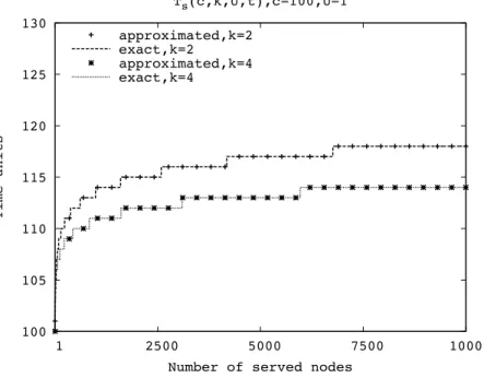
The derived bound explicitly accounts for the fact that each node at most can feed k neighbors. If this restriction is removed, we obtain a more simple and immediate expression N(t) = U ' j=1 S∞(t− j + 1) = U ' j=1 2t−j = 2t(1− 2−U) (2.24) We can compare the results given by the approximation formula and the exact solution. Figure 2.3 shows the time T (n) needed by n peer nodes to complete the download of the 100-th chunk as a function of the number n of peer nodes and for two values of the number k of parents/children. We observe that the asymptotic approximate expression tends to be exact for large values of t but is fairly accurate already for very small values of t.
The same behavior can be observed in figure 2.4, which shows the maximum number of peer nodes N(t) that can complete the download of the 100-th chunk as a function of the time t and for two values of the number k of parents/children.
100 105 110 115 120 125 130 10000 7500 5000 2500 1 Time units
Number of served nodes Ts(c,k,U,t),c=100,U=1 approximated,k=2
exact,k=2
approximated,k=4 exact,k=4
Figure 2.3. Asymptotic and exact evaluation of the time units needed by n peer nodes to complete the download of the 100-th chunk as a function of the number
n of peer nodes, and for two values of k.
100 105 1010 1015 1020 1025 1030 200 180 160 140 120 100
Number of served nodes
Time units approximated, k=2 exact, k=2 approximated, k=4 exact, k=4
Figure 2.4. Asymptotic and exact evaluation of the maximum number of peer nodes that can complete the download of the 100-th chunk as a function of the
2.4
Attaining the bound
The provided bound offers only limited insights on how chunks should be forwarded across the overlay topology. Specifically, the bound clearly suggests that delay performances are optimized only if chunks are serially delivered towards the neighbor nodes, but does not make any assumption on which specific paths the chunks should follow, or in other words, which overlay topologies should be used. We now show that, to attain the performance bound, peer nodes have to be organized according to i) an overlay unbalanced tree if k = U, ii) multiple overlay unbalanced trees if k > U and multiple of U
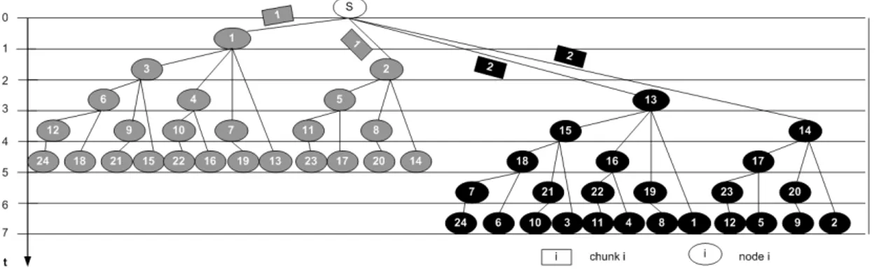
When the number of neighbor nodes k is equal to the normalized upload capacity U, the source node can deliver each chunk to all its k neighbors before a new chunk arrives. As such, the source node can repeatedly apply a round-robin scheduling policy during the time interval T = UT∗, which elapses between the arrivals of consecutive chunks. Specifically, in the first T∗ seconds it can send a given chunk to a given node, say peer N1, then send the chunk to peer N2, and so on until peer Nk. If this policy is repeated for every chunk, the result is that any neighbor of the source also receives a new chunk every T = UT∗ seconds. Hence, each neighbor of the source may apply the same scheduling policy with respect to its neighbors, and so on. As a consequence, every node in the network receives chunks from the same parent, and in the original order of generation: in other words, chunks are delivered over a tree topology.
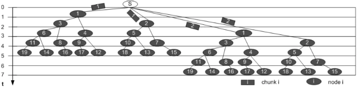
Figure 2.5. Overlay tree resulting in the case k = U = 2.
The operation of the above described chunk distribution mechanism is depicted in figure 2.5, which refers to the case U = k = 2 and a network composed of 19 nodes. In this figure the source is denoted with an “S”. The nodes and the chunks
are progressively indexed starting from 1. Going from the upper part of the figure to its lower part, we see how the first two chunks are progressively distributed starting from the source; the time since the start of the transmission, measured in time units, until time instant t = 7 is reported on the left side of the figure. The tree on the left hand side of the figure distributes the first chunk, while the tree on the right hand side of the figure distributes the second chunk. In more detail, since the first chunk is assumed to be available for transmission at the source at time instant t = 0, the source starts transmitting the first chunk to node 1 at t = 0 and after finishing this transmission, i.e at t = 1, it sends the first chunk to node 2, in series. In its turn, node 1 sends the first chunk first to node 3 and then to node 4, in series, and so on. Likewise, node 2 sends the first chunk first to node 5 and then to node 7, in series, and so on. As regards the second chunk, the source starts transmitting it to node 1 at time t = 2, exactly when that chunk is available for the transmission. After finishing transmitting the first chunk to node 1, the source sends the same chunk to node 2, in series. In their turn, node 1 and 2 distribute the second chunk in same manner as the first chunk, i.e. sending the second chunk in series first to nodes 3 and 5 respectively, and then to nodes 4 and 7 respectively.
It is to be noted that, even if two distribution trees are depicted in figure 2.5, actually there is only one distribution, which repeats itself for each chunk with period k = U = 2. In other words, a given node receives all chunks through the same path. It is also interesting to note that the tree formed in figure 2.5 is unbalanced in terms of number of hops. For instance, the first chunk reaches node 19 at time t = 5 after crossing nodes 1,3,6 and 11. Conversely, the same chunk reaches node 15, again at time t = 5, after crossing nodes 2 and 7. The unbalancing in terms of number of hops is a consequence of the fact that the proposed approach achieves equal-delay source-to-leaves paths, and that the time in which a chunk waits for its transmission turn at a node (because of serialization) contributes to such path delay.
We are now in condition to evaluate the stream diffusion metric N(t). To this end, let us introduce n(i) as number of new nodes that complete the download of a chunk exactly i time units after the generation of that chunk at the source node, in such a way that N(t) can be assessed according to the equation N(t) = %t
i=1n(i). With reference to figure 2.5, n(1) = 1 (node 1), n(2) = 2 (nodes 2 and 3), n(3) = 3 (nodes 4, 5 and 6), n(4) = 5 (nodes 7, 8, 9, 10 and 11), n(5) =