SOME RESULTS ON A GENERALIZED RESIDUAL ENTROPY
BASED ON ORDER STATISTICS
Suchandan Kayal1
Department of Mathematics, National Institute of Technology Rourkela, Rourkela-769008, India
1. Introduction
To quantify the statistical nature of lost information in communication channels mathematically, Shannon (1948) introduced a concept (known as the Shannon en-tropy) analogous to the entropy described in statistical thermodynamics. Let X be a non-negative random variable representing the lifetime of a component with an absolutely continuous cumulative distribution function (CDF) F (x), probabil-ity densprobabil-ity function (PDF) f (x), survival function (SF) ¯F (x) = 1− F (x) and hazard rate (HR) λF(x) = f (x)/ ¯F (x). The Shannon entropy of X is given by S(X) =−∫0∞f (x) ln f (x)dx, which has received considerable popularity in a wide variety of contexts. For a detailed account of importance and applications of the notion of entropy in various disciplines one may refer to Cover and Thomas (2006). The Shannon entropy S(X) can be seen as a negative logarithm moment as it is expectation of logarithm of the fundamental measure with a negative sign. As different moments divulge different information on the distribution, it is expected that other entropies (generalized) may divulge different characteristics of the data set. Due to this reason, several general families of entropy measures have been introduced in the literature. In this direction we refer to Renyi (1961); Varma (1966); Kapur (1967); Tsallis (1988). Note that these generalized measures have several properties such as smoothness, large dynamic range with respect to certain conditions that make them useful for specific applications (see for example, Varma, 1966; Renyi, 2012; Tsallis, 1988; Kapur, 1994). Pharwaha and Singh (2009) de-termined randomness of mammograms based on some non-Shannon measures as these have higher dynamic range than the Shannon measure over a variety of scattering conditions and therefore, useful in the problems of estimating scatter density and regularity (see Smolikovd et al., 2002). For a non-negative random variable X, the generalized entropy (see Varma, 1966) of order (α, β) is given by
Vα,β(X) = ( 1 β− α ) ln ∫ ∞ 0 fα+β−1(x)dx, 0≤ β − 1 < α < β. (1)
Note that as β equals to 1, (1) reduces to the Renyi entropy of order α (see Renyi, 1961) of a non-negative random variable X.
In the context of reliability and life testing studies when the present age of a component needs to be incorporated, the measure given in (1) is not appropriate. In this situation one may be interested in studying the residual lifetime of a com-ponent which is still working at time t≥ 0. We denote it by Xt= [X− t|X ≥ t]. Accordingly, the measure Vα,β(X) given in (1) needs to be modified. For some ref-erences on residual entropy and generalized residual entropy, we refer to Ebrahimi and Pellerey (1995); Ebrahimi (1996); Ebrahimi and Kirmani (1996); Belzunce et al. (2004); Abraham and Sankaran (2005); Nanda and Paul (2006); Zarezadeh and Asadi (2010); Li and Zhang (2011). In analogy to Ebrahimi (1996), a gener-alized residual entropy (GRE) of order (α, β) of X is given by
Vα,β(X; t) = ( 1 β− α ) ln ∫ ∞ t fα+β−1(x) ¯ Fα+β−1(t)dx, 0≤ β − 1 < α < β, t ≥ 0. (2) It is noted that when t = 0, Vα,β(X; t) reduces to Vα,β(X). The measure (2) plays an important role as a measure of complexity and uncertainty in different areas such as physics, electronics and engineering to describe many chaotic systems. In actuarial science, GRE given in (2) can be presented as the pre-payment entropy of claims (losses) with a deductible t. For some results on information measures based on (1), we refer to Kayal and Vellaisamy (2011); Kumar and Taneja (2011); Kayal (2015a,b). In this paper, we investigate some properties of GRE of order statistics. It is noted that order statistics specially deal with the properties and applications of ordered random variables and their functions. In the study of many real life problems related to flood, breaking strength, atmospheric temperature, atmospheric pressure etc., the future possibilities in the recurrence of extreme sit-uations are of much importance and accordingly, the problem of interest in these cases reduces to that of the extreme observations. Besides these, the order statis-tics have been applied in several domains, such as in robust statistical estimation and detection of outliers, digital image processing, characterization of probability distributions, entropy estimation, reliability analysis. For detail, one may refer to David and Nagaraja (2003) and the references therein.
In Section 2, we present some preliminary results. We establish that both increasing generalized residual entropy (IGRE) and decreasing generalized residual entropy (DGRE) properties of a stochastically smaller random variable is preserved by the larger one in Section 3. It is shown that IGRE and DGRE properties are preserved by the formation of a parallel system, but not under the formation of a series system. We obtain bounds for GRE of order statistics. Under some conditions, we establish that the GRE of parallel and series systems are monotone functions of the number of observations of a sample. Finally, in Section 4, we present some computational results to verify some of the results derived in Section 3. We also provide estimators in estimating the GRE of exponential distribution. The maximum likelihood estimator is derived in this purpose.
Throughout the paper, we assume that the random variables are non-negative and have absolutely continuous CDF. The terms decreasing and increasing are used for non-increasing and non-decreasing, respectively. We denote γ = α + β− 1,
where 0≤ β − 1 < α < β.
2. Background
Here, we present some preliminaries which will be required to obtain some results in the rest of the paper. Let X1, X2, . . . , Xr, . . . , Xn be n independent copies of a random variable X with absolutely continuous CDF F (x) and PDF f (x). The order statistics of{X1, X2, . . . , Xr, . . . , Xn} are defined as an arrangement of the observations in increasing order. We denote X1:n ≤ X2:n ≤ . . . ≤ Xr:n ≤ . . . ≤ Xn:n, where Xr:n represents the r-th order statistic. Order statistics have various applications. For example, a policy for a couple pays out when the first of the spouses dies. Here one’s interest may be on studing the distribution of X1:n, which
is the random variable defined to be the minimum of two lifespans of the couple. Also, let an insurance company hold 500 policies of which somebody has cash-at-hand to pay 250. In this set up, one may be interested to know the distribution of the variable X250:500, the 250th occurrence of a pay-out. The PDF and SF of Xr:n are respectively given by
fr:n(x) = 1 B(r, n− r + 1)F r−1(x) ¯Fn−r(x)f (x) (3) and ¯ Fr:n(x) = r−1 ∑ i=0 ( n i ) Fi(x) ¯Fn−i(x) =BF (x)(r, n− r + 1) B(r, n− r + 1) , (4)
where B(a, b) =∫01ua−1(1−u)b−1du, a > 0, b > 0 and B
F (x)(a, b) = ∫1
F (x)u a−1(1− u)b−1du, a > 0, b > 0. Here, B(a, b) and BF (x)(a, b) are known as beta function and incomplete beta function, respectively. For a > 0 and b > 0, we denote the truncated beta distribution as Bt(a, b). Let Y be a random variable following Bt(a, b) distribution (denoted by Y ∼ Bt(a, b)), then the PDF of Y is
fY(x) =
xa−1(1− x)b−1 Bt(a, b)
, t < x < 1, a > 0, b > 0. (5)
The HR of Xr:n can be written as λFr:n(x) =
n!
(r− 1)!(n − r)!∑ri=0−1(ni)(F (x)/ ¯F (x))i−(r−1)λF(x). (6) Let X be a random variable following uniform distribution with PDF
f (x|a, b) = 1
b− a, 0 < a < x < b. For convenience, we denote X ∼ U(a, b).
Lemma 1. (Thapliyal and Taneja, 2012) Let Ur:nbe the r-th order statistic of a random sample of size n from U (0, 1). Then
Vα,β(Ur:n; t) = ( 1 β− α ) ln Bt(γ(r− 1) + 1, γ(n − r) + 1) −( γ β− α ) ln Bt(r, n− r + 1). (7)
Lemma 2. (Thapliyal and Taneja, 2012) Let X be a random variable with CDF F (x) and PDF f (x). Then GRE of the r-th order statistic can be represented in terms of that of the r-th order statistic from U (0, 1) as
Vα,β(Xr:n; t) = Vα,β(Ur:n; F (t)) + ( 1 β− α ) ln E[fγ−1(F−1(Yr))], (8) where Yr∼ BF (t)(γ(r− 1) + 1, γ(n − r) + 1).
Let X and Y denote the random variables with respective CDFs F (x) and G(x), PDFs f (x) and g(x), SFs ¯F (x) and ¯G(x) and HRs λF(x) and λG(x).
Definition 3. A random variable X has decreasing (increasing) generalized residual entropy of order (α, β), abbreviated by DGRE (IGRE) if Vα,β(X; t) is decreasing (increasing) in t≥ 0.
Definition 4. A random variable X is said to be stochastically less than or equal to Y, abbreviated by X
st
≤ Y, if F (t) ≤ G(t), for all t ≥ 0.
Definition 5. A random variable X is said to be less than or equal to Y in likelihood ratio ordering, abbreviated by X≤ Y, if f(t)/g(t) is decreasing in t ≥ 0.lr Note that when the supports of X and Y have a common left end point, we have the following result between the stochastic order and the likelihood ratio order described in Definition 4 and Definition 5, respectively.
X≤ Y ⇒ Xlr ≤ Y.st
One may refer to Shaked and Shanthikumar (2007) for more results on usual stochastic orderings.
3. Main Results
We begin with the following lemma which will be used in obtaining new results in this section.
Lemma 6. The GRE of a random variable X with CDF F (x) and PDF f (x) can be expressed as Vα,β(X; t) = (1− γ β− α ) ln ¯F (t) + ( 1 β− α ) ln E[fγ−1(X)|X ≥ t] = − ( ln γ β− α ) + ( 1 β− α ) ln E[λγF−1(Xγ)|Xγ≥ t],
where λF(x) = f (x)/ ¯F (x) is the hazard rate function of X and Xγ has the survival function ¯Fγ(x).
Proof. From (2) we have Vα,β(X; t) = ln ¯F (t) + ( 1 β− α ) ln ∫ ∞ t [ fγ(x) ¯ F2β−1(t) ] dx = (1− γ β− α ) ln ¯F (t) + ( 1 β− α ) ln ∫ ∞ t fγ−1(x)f (x)¯ F (t)dx = (1− γ β− α ) ln ¯F (t) + ( 1 β− α ) ln E[fγ−1(X)|X ≥ t],
since the distribution of [X|X ≥ t] is f(x)/ ¯F (t). To prove the second part, again from (2) Vα,β(X; t) = − ( ln γ β− α ) + ( 1 β− α ) ln ∫ ∞ t fγ−1(xγ) ¯ Fγ−1(x γ) f (xγ|xγ ≥ t)dxγ = − ( ln γ β− α ) + ( 1 β− α ) ln E[λγF−1(Xγ)|Xγ≥ t].
This completes the proof. 2
In the following we obtain expressions of Vα,β(X; t), Vα,β(X1:n; t) and Vα,β(Xn:n; t)
for exponential and Pareto distributions.
Example 1. Exponential distribution has prominent applications in various real life problems. For example, service times, inter-arrival times, etc. are usually observed to be exponentially distributed. Let X be a random variable following exponential distribution with CDF F (x|σ) = 1 − exp(−σx), x > 0, σ > 0. It is easy to obtain that Vα,β(X; t) = −(β−α1 ) ln γ + (βγ−α−1) ln σ. Now, to compute Vα,β(Xr:n; t), we have f (F−1(x)) = σ(1−x) and E[fγ−1(F−1(Y1))] = (((n−1)γ +
1)σγ−1/nγ) exp(−σt(γ − 1)). Again V
α,β(X1:n; t) =−(β−α1 ) ln γ + (βγ−α−1) ln(nσ). For r = n, from Lemma 2, we obtain Vα,β(Xn:n; t) = (βγ−α−1) ln σ−(β−αγ ) log(1n(1− (F (t|σ))n)) + ( 1
β−α) log ∫1
F (t|σ)x
γ(n−1)(1− x)γ−1dx.
Example 2. Pareto distribution plays a central role in various applications. It is used in the investigation of city population, occurrence of natural resources, insurance risk and business failures. It has been an important model in many socio-economic studies. Let X be a random variable following Pareto distribu-tion with CDF F (x|θ, δ) = 1 − (δ/x)θ, x ≥ δ > 0, θ > 0. Now, it is easy to obtain that f (F−1(x)) = θ(1− x)1+1 θ/β and E[fγ−1(F−1(Y1))] = [(γ(n− 1) + 1)/(γ(nθ + 1)− 1)](δ/t)(θ+1)(γ−1)θγδ1−γ. We obtain V α,β(X; t) = −(βγ−α−1) ln t + (β−αγ ) ln θ− (β−α1 ) ln[γ(θ + 1)− 1], provided γ > (θ + 1)−1. Again, Vα,β(X1:n; t) = −(γ−1 β−α) ln t+( γ β−α) ln(nθ)−( 1 β−α) ln[γ(nθ +1)−1], provided γ > (nθ+1)−1. Also, from Lemma 2, Vα,β(Xn:n; t) =−(βγ−α−1) ln(θ/δ)−(β−αγ ) ln((1−(1−(δ/t)θ)n)/n) + (β−α1 ) ln∫11−(δ/t)θ(1− x) (θ+1)(γ−1) θ xγ(n−1)dx.
Now, we present some results on GRE in terms of ordering properties of distri-butions. Several aging properties can be characterized in reliability theory using stochastic comparison between total and its residual lifetime. For example, new better than used property holds if and only if Xt≤ X, for all t ≥ 0. In the followingst theorem we prove a similar characterization of DGRE distributions.
Theorem 7. A random variable X with PDF f (x) and SF ¯F (x) is DGRE if and only if Vα,β(Xs; t)≤ Vα,β(X; t), for all s, t≥ 0.
Proof. A random variable X is DGRE if and only if Vα,β(X; s+t)≤ Vα,β(X; t), for all s, t≥ 0. Moreover, the PDF and SF of Xsare given as fs(x) = f (s+x)/ ¯F (s) and ¯Fs(x) = ¯F (s + x)/ ¯F (s), respectively. Therefore, for all s, t≥ 0,
Vα,β(Xs; t) = ( 1 β− α ) ln ∫ ∞ t fsγ(x) ¯ Fsγ(t) dx = ( 1 β− α ) ln ∫ ∞ s+t fγ(x) ¯ Fγ(s + t)dx = Vα,β(X; s + t).
This completes the proof. 2
2 3 4 5 -4 -3 -2 -1 1 2 3 (a)
Figure 1 – Plot of Vα,β(X; s + t) (bottom curve) and Vα,β(X; t) (top curve) versus t (along horizontal axis) for Pareto distribution as described in Example 2. Here we assume
α = 1.2, β = 1.5, θ = 2 and s = 1.
From Fig. 1, it is easy to see that the Pareto random variable is DGRE for α = 1.2, β = 1.5 and θ = 2. Here, it should be mentioned that we observe similar behaviour of Pareto distribution for any θ > 0 and α + β > 2. Our next theorem is a key result to obtain some subsequent results.
Theorem 8. Let X and Y be two random variables with CDFs F (x) and G(x), PDFs f (x) and g(x), SFs ¯F (x) and ¯G(x) and HRs λF(x) and λG(x), respectively. Also let X≤ Y ; and λlr G(t)/λF(t) be an increasing function in t≥ 0. If X is IGRE (DGRE), then Y is also IGRE (DGRE).
Proof. Assume ξ(t) = λG(t)/λF(t). Then from Lemma 6, the GRE of Y can be written as Vα,β(Y ; t) =− ( ln γ β− α ) + ( 1 β− α ) ln E[λγF−1(Yγ)ξγ−1(Yγ)|Yγ ≥ t]. (9)
Under the given assumption, it is required to show that η(t) = E[λγF−1(Yγ)ξγ−1(Yγ) |Yγ ≥ t] is increasing (decreasing) in t ≥ 0, that is, η′(t) = γλG(t)[η(t) − λγF−1(t)ξγ−1(t)] ≥ (≤)0, where ′ denote the derivative. The PDF of [Yγ|Yγ ≥ t] can be obtained as f (yγ|yγ ≥ t) = γ ¯Gγ−1(yγ)g(yγ) ¯ Gγ(t) , yγ≥ t. Moreover, η(t)− λγF−1(t)ξγ−1(t) = ∫ ∞ t f (yγ|yγ ≥ t)[λγF−1(yγ)ξ γ−1(yγ)− λγ−1 F (t)ξ γ−1(t)]dyγ = ∫ ∞ t f (yγ|yγ ≥ t)ξγ−1(yγ)[λ γ−1 F (yγ)− λ γ−1 F (t)]dyγ + ∫ ∞ t f (yγ|yγ ≥ t)λ γ−1 F (t)[ξ γ−1(y γ)− ξγ−1(t)]dyγ = I1+ I2, where I1= ∫∞ t f (yγ|yγ ≥ t)ξ γ−1(yγ)[λγ−1 F (yγ)−λ γ−1 F (t)]dyγand I2= ∫∞ t f (yγ|yγ ≥ t)λγF−1(t)[ξγ−1(yγ)− ξγ−1(t)]dyγ. Let X be IGRE (DGRE), implies Vα,β(X; t) be an increasing (decreasing) function in t≥ 0. Thus, h(t) = E[λγF−1(Xγ)|Xγ ≥ t] is also an increasing (decreasing) function in t ≥ 0. Therefore, we have h(t) ≥ (≤ )λγF−1(t), which implies that
∫ ∞ t
γf (xγ) ¯Fγ−1(xγ)[λFγ−1(xγ)− λγF−1(t)]dxγ ≥ (≤)0, (10)
for all t ≥ 0. Again under the assumption X≤ Y, and using Lemma 7.1(a) oflr Barlow and Proschan (1981), it can be shown that
I1= 1 ¯ Gγ(t) ∫ ∞ t gγ(yγ) fγ(y γ)
γ ¯Fγ−1(yγ)f (yγ)[λγF−1(yγ)− λγF−1(t)]dyγ≥ (≤)0. Moreover, as ξ(t) is an increasing function in t≥ 0, therefore it can also be shown
that I2≥ (≤)0. This completes the proof. 2
In recent years, researchers in reliability theory have shown considerable at-tention in the study of stochastic and reliability properties of various technical systems. The (n− r + 1)-out-of-n system structure is a very popular type of redundancy. This system functions if and only if at least (n− r + 1) out of n components are operating (r≤ n). In particular, when r = 1 and r = n, it corre-sponds to series and parallel system, respectively. The GRE of Xr:nmeasures the
entropy of the residual lifetime of a (n− r + 1)-out-of-n working system at time t ≥ 0. Hence, it can be important for system designers to get information about the entropy of used (n− r + 1)-out-of-n systems at any time t ≥ 0. Asadi and Ebrahimi (2000) established that decreasing uncertainty residual life is preserved under the formation of parallel system. Recently, Mahmoudi and Asadi (2010) and Li and Zhang (2011) showed that decreasing Renyi entropy residual life property is preserved under the formation of the same system. It is not difficult to show that fn:n(x)/f (x) and λFn:n(x) λF(x) = n n∑−1 i=0 ( n i )(F (x) ¯ F (x) )i−(n−1)
are increasing in x≥ 0. Hence, as a consequence of Theorem 8, we get the following corollary which shows that IGRE and DGRE properties of the life distributions are preserved under the formation of parallel system.
Corollary 9. Let X be a random variable as described in Theorem 8. Then the n-th order statistic Xn:n is IGRE (DGRE) if X is.
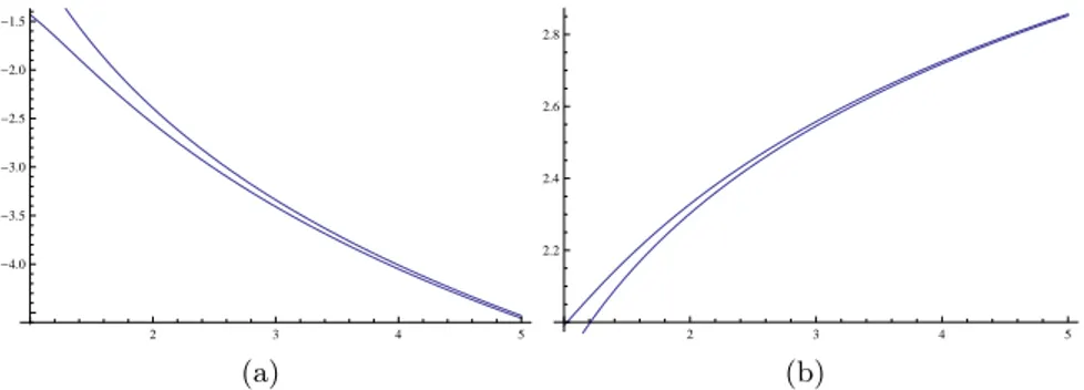
As an application of Corollary 9, we consider the example presented in Fig. 2 which shows that IGRE and DGRE properties of Pareto distributions are pre-served under the formation of parallel system.
2 3 4 5 -4.0 -3.5 -3.0 -2.5 -2.0 -1.5 (a) 2 3 4 5 2.2 2.4 2.6 2.8 (b)
Figure 2 – (a) Plot of Vα,β(Xn:n; t) (bottom curve) and Vα,β(X; t) (top curve) versus
t (along horizontal axis) for Pareto distribution as described in Example 2. Here we
assume α = 1.2, β = 1.5, θ = 2, δ = 0.2 and n = 5. (b) Plot of Vα,β(Xn:n; t) (top curve) and Vα,β(X; t) (bottom curve) versus t (horizontal axis) for Pareto distribution. Assume
α = 0.2, β = 1.2, θ = 2, δ = 0.2 and n = 5.
The following example shows that DGRE and IGRE properties do not hold under the formation of a series system.
Example 3. Suppose a random variable X has the SF ¯ F (x) = 1−x 2 2 , 0≤ x < 1, 2 3 − x2 6 , 1≤ x < 2, 1, x≥ 2. (11)
The GRE of X and the first order statistic X1:ncan be obtained as
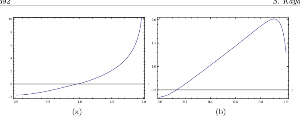
Vα,β(X; t) = ( 1 β− α ) ln [( 2 2− t2 )γ(1− tγ+1 γ + 1 + 2γ+1− 1 (γ + 1)3γ )] , if 0≤ t < 1, ( 1 β− α ) ln [( 2 4− t2 )γ(2γ+1− tγ+1 γ + 1 )] , if 1≤ t < 2, (12) and Vα,β(X1:n; t) = ( 1 β− α ) ln [ (2n)γ (2− t2)nγ ∫ 1 t ( x(2− x2)n − 1 )γ dx + (3n)γ (3(2− t2))nγ ∫ 2 1 ( x(4− x2)n − 1)γdx ] , if 0≤ t < 1, ( 1 β− α ) ln [ (2n)γ (4− t2)nγ ∫ 2 t ( x(4− x2)n − 1)γdx ] , if 1≤ t < 2, (13) respectively. 0.0 0.5 1.0 1.5 2.0 -2.0 -1.5 -1.0 -0.5 0.0 0.5 t (a) 0.0 0.2 0.4 0.6 0.8 1.0 -0.6 -0.5 -0.4 -0.3 -0.2 -0.1 t (b)
Figure 3 – (a) V0.4,1.2(X; t) Vs t, (b) V0.4,1.2(X1:n; t) Vs t when n = 10.
From Fig. 3(a), it is clear that Vα,β(X; t) given in (12) is decreasing in t, for α = 0.4 and β = 1.2, that is, X is DGRE, but Vα,β(X1:n; t) (see Fig. 3(b)) is
not monotone in 0≤ t < 1, for the same values of α and β, when n = 10. Hence, we conclude that X1:n is not DGRE. Also Fig. 4(a) shows that Vα,β(X; t) is increasing in t for α = 1.1 and β = 1.2, that is, X is IGRE, whereas Vα,β(X1:n; t)
0.0 0.5 1.0 1.5 2.0 -2 0 2 4 6 8 10 t (a) 0.0 0.2 0.4 0.6 0.8 1.0 0.5 1.0 1.5 2.0 t (b)
Figure 4 – (a) V1.1,1.2(X; t) Vs t, (b) V1.1,1.2(X1:n; t) Vs t when n = 10.
is not monotone in 0≤ t < 1, for the same values of α, β and n = 10 (see Fig. 4(b)).
Asadi and Ebrahimi (2000) proved that if Xr:nis decreasing uncertainty resid-ual life, then Xr+1:n, Xr:n−1and Xr+1:n+1are also decreasing uncertainty residual life. Li and Zhang (2011) proved it for the Renyi entropy. In the following corol-lary, we establish a similar result for GRE given in (2).
Corollary 10. Let X be a random variable as described in Theorem 8. Then the order statistics Xr+1:n, Xr:n−1 and Xr+1:n+1 are IGRE (DGRE) if Xr:nis.
Proof. Using the results of Nagaraja (1990) and the Theorem 8, the proof
follows. 2
In the following we obtain bounds for the GRE of the r-th order statistic in terms of the GRE of each components and that of the r-th order statistic from U (0, 1). Note that the bounds are useful when the GRE of order statistics does not have a closed form expression, or the expectation in Lemma 2 can not be easily evaluated.
Theorem 11. Let X be a random variable as described in Theorem 8. Also let Vα,β(X; t) and Vα,β(Xr:n; t) denote the GREs of X and Xr:n, respectively. Then the following results hold.
(a) Let Vα,β(X; t) be finite. If Mr= max{F (t),rn−1−1}, then Vα,β(Xr:n; t)≤ Vα,β(X; t) + ( γ β− α ) ln ¯F (t) + Ar(t), (14) where Ar(t) = ( γ β−α ) [(r− 1) ln Mr+ (n− r) ln(1 − Mr)− ln BF (t)(r, n− r + 1)]. (b) Let M = f (m) be finite, where m = sup{x : f(x) ≤ M} is mode of the distribution. Then Vα,β(Xr:n; t)≤ (≥)Vα,β(Ur:n; F (t)) + (γ− 1 β− α ) ln M, for α + β > (<)2. (15)
Proof. (a): From (8) we have Vα,β(Xr:n; t) = Vα,β(Ur:n; F (t)) + ( 1 β− α ) ln ∫ 1 F (t) yγ(r−1)(1− y)γ(n−r)fγ−1(F−1(y)) BF (t)(γ(r− 1) + 1, γ(n − r) + 1) dy ≤ Vα,β(Ur:n; F (t)) + ( 1 β− α ) ln ( Mr ∫ 1 F (t) fγ−1(F−1(y))dy ) = Vα,β(Ur:n; F (t)) + ( 1 β− α ) ln ∫ 1 t fγ(v)dv + ( 1 β− α ) ln Mr = Vα,β(Ur:n; F (t)) + Vα,β(X; t) + ( 1 β− α ) ln( ¯Fγ(t)Mr) = Vα,β(X; t) + ( γ β− α ) ln ¯F (t) + Ar(t).
This completes the proof of Part (a). The proof of Part (b) follows as fγ−1(F−1(y))≤
(≥)Mγ−1, for α + β > (<)2. 2
In the following we obtain bounds of GRE of the r-th order statistic for Pareto and generalized exponential distributions.
Example 4. (a) Let X be a random variable with PDF f (x|θ, δ) = θδ
θ xθ+1, x≥ δ > 0, θ > 0. Then Vα,β(Xr:t; t)≤ Ar(t) + (β−α1 ) ln[ (θδ θ)γ (γ(θ+1)−1)tγ(θ+1)−1] and Vα,β(Xr:t; t)≤ (≥)Vα,β(Ur:n; F (t)) + (βγ−1−α) ln( θ δ), for α + β > (<)2.
(b) For a random variable with PDF f (x|θ) = θe−x(1− e−x)θ−1, x > 0, θ > 0, we have Vα,β(Xr:t; t)≤ Ar(t) + (β−α1 ) ln[θγB¯1−e−t(γ(θ−1)+1, γ)] and Vα,β(Xr:t; t)≤
(≥)Vα,β(Ur:n; F (t)) + (βγ−α−1) ln(1−1θ)θ−1, θ > 1, for α + β > (<)2.
In this part of the paper we obtain some monotone properties of GRE of parallel and series systems. First we present the following theorem, which will be helpful to obtain further results.
Theorem 12. Let u(x) and vλ(x), λ > 0 be non-negative functions, where u(x) is increasing. Assume that 0≤ t < c ≤ ∞ and Wλ has a density function fWλ(w), where fWλ(w) = upλ(w)v λ(w) ∫c t upλ(x)vλ(x)dx , t < w < c, p∈ R. (16)
For p∈ R, we define a function hγ(.) as
hγ(p) = ( 1 β− α ) ln ∫c t u pγ(x)v γ(x)dx ( ∫c t up(x)v1(x)dx )γ. (17) Then for Wγ st
Proof. Assume that hγ(p) is differentiable. Therefore we have ∂hγ(p) ∂p = γ( ∫tcup(x)v 1(x)dx )−(γ+1) (β− α)gγ(p) [ ∫ c t ln u(x)upγ(x)vγ(x)dx ∫ c t up(x)v1(x)dx − ∫ c t ln u(x)up(x)v1(x)dx ∫ c t upγ(x)vγ(x)dx ] , (18) where gγ(p) = ∫c t u pγ(x)v γ(x)dx/ ( ∫c t u p(x)v 1(x)dx )γ
. Using the fact that Wγ st
≤ (≥ )Wst 1
and ln is increasing function we get (see Shaked and Shanthikumar, 2007)
E[ln u(Wγ)]≤ (≥)E[ln u(W1)], (19)
which implies that (18) is non-positive (non-negative). Hence hγ(p) is a decreasing
(increasing) function of p. This completes the proof. 2
Theorem 13. Under the assumptions of Theorem 12, if u(x) is decreasing, then for Wγ
st
≤ (≥ )Wst 1, hγ(p) is an increasing (decreasing) function of p.
Proof. The proof is similar to that of the Theorem 12, hence omitted. 2 In consequence of the Theorem 12 and Theorem 13, we have the following corollary.
Corollary 14. Consider a parallel (series) system consists of n components from U (0, 1). Then the GRE of the system lifetime (Un:n(U1:n)) is increasing (de-creasing) function of the number of components for α + β > (<)2.
Proof. From (7), we have Vα,β(Un:n; t) = (β−α1 ) ln(∫t1xγ(n−1)dx/(∫t1xn−1dx)γ), which can be written in the form of (17), where u(x) = x and vγ(x) = x−γ. With-out loss of generality, one may assume that n≥ 1 is a continuous variable. Also, it can be showed that the ratio∫t1xγ(n−1)dx/∫t1xn−1dx is increasing (decreasing) for α + β > (<)2. Thus, for the chosen functions u(x) = x and vγ(x) = x−γ, it is easy to prove that Wγ
st
≥ (≤ )Wst 1, for α + β > (<)2, where the density function
of Wλ is given in (16). Therefore, from Theorem 12, the proof follows for parallel system. The proof for a series system follows similarly. This completes the proof. 2 Corollary 15. Let Ur:n denote the r-th order statistic of U (0, 1). If r1 ≤ r2≤ n are integers then for t ≥ rn2−1−1, Vα,β(Ur1:n; t)≤ Vα,β(Ur2:n; t).
Proof. From (7), Vα,β(Ur:n; t) can be written as Vα,β(Ur:n; t) = ( 1 β− α ) ln ( ∫ 1 t urγ(x)vγ(x)dx /[ ∫ 1 t ur(x)v1(x)dx ]γ) , (20) where u(x) = x/(1− x) and vγ(x) = (1− x)rγ/xγ. Again, for α + β > (<)2 and t≥ r−1
n−1, it is not hard to see that Wγ st
≥ (st≤ )W1. Therefore, for r1≤ r2≤ n and t≥r2−1
In the following we obtain some results for the random variables having mono-tone density functions. Note that the class of CDFs with decreasing PDF contains exponential, Pareto, mixture of exponential and Pareto distributions, etc. There are also CDFs with increasing PDF. For example the power distribution with PDF f (x|a) = axa−1, 0 < x < 1, a > 0 has increasing density function.
Theorem 16. Consider a parallel (series) system consists of n components with CDF F (x) and PDF f (x). Further, assume that f (x) is increasing (decreas-ing) in its support. Then the GRE of a system lifetime is increasing (decreas(decreas-ing) in n for α + β > (<)2.
Proof. First we prove the result for parallel system. The other part follows analogously. Assume Yn ∼ BF (t)(γ(n− 1) + 1, 1). Then it can be easily shown that Yn≤ Yst n+1. Also, for α + β > (<)2, fγ−1(F−1(x)) is increasing (decreasing) in x. Hence for α + β > (< 2), ( 1 β− α ) lnE(f γ−1(F−1(Yn+1))) E(fγ−1(F−1(Y n))) ≥ (≤)0. (21)
Moreover, from Lemma 2 we have
Vα,β(Xn+1:n+1; t)− Vα,β(Xn:n; t) = δα,β(n; t)− ( 1 β− α ) ln [ E[fγ−1(F−1(Yn))] E[fγ−1(F−1(Yn+1))] ] , where δα,β(n; t) = Vα,β(Un+1:n+1; F (t))− Vα,β(Un:n; F (t)). Now using Corollary 14 and the inequality (21) the proof follows. This completes the proof. 2
0 1 2 3 4 5 7.5 8.0 8.5 9.0 9.5 10.0 10.5 11.0 (a) 1 2 3 4 5 10 11 12 13 14 15 (b)
Figure 5 – Fig. (a) and (b) represent plot of Vα,β(Xn:n; t) of exponential distribution with mean 1 and 0.5, respectively. Assume α = 1.2 and β = 1.5. Curves corresponds to sample sizes 5, 10, 15, 20, 30 are from bottom to top.
4. Computation Results
In this section, we show that some of the results derived in the earlier sections of this paper are consistent with the numerical study. We present the estimated value
of Vα,β(X; t), Vα,β(X1:n; t) and Vα,β(Xn:n; t) of an exponential distribution with mean 1/σ, σ > 0. It should be mentioned that the statistical data are generated based on the Monte-Carlo simulation. The estimated values are computed based on 5000 samples with different sample sizes and different values of the parameters. The generalized residual entropy of exponential distribution with mean 1/σ can be obtained as Vα,β(X; t) = ( 1 β− α ) ln(σγ−1/γ). (22)
To estimate Vα,β(X; t) given in (22) from simulated exponential data, we use the maximum likelihood estimator (MLE) of σ. Let X1, X2, . . . , Xn be a random sample drawn from exponential distribution with mean 1/σ. Then the maximum likelihood estimator of σ is given by ˆσml = n/
∑n
i=1Xi = 1/ ¯X. As MLE is in-variant, therefore for exponential distribution, Vα,β(X; t) can be estimated via the MLE which is given by
ˆ Vα,β(X; t) = ( 1 β− α ) ln ((1/ ¯X)γ−1 γ ) . (23)
The generalized residual entropy of X1:nand Xn:nof exponential distribution can
be obtained as Vα,β(X1:n; t) = ( 1 β− α ) ln ((nσ)γ−1 γ ) (24) and Vα,β(Xn:n; t) = (γ− 1 β− α ) ln σ− ( γ β− α ) log (1 n ( 1− (F (t))n )) + ( 1 β− α ) log ∫ 1 F (t) xγ(n−1)(1− x)γ−1dx, (25)
respectively, where F (t) = 1− exp(−σt). The estimators of Vα,β(X1:n; t) and Vα,β(Xn:n; t) given in (23) and (24), are given by
ˆ Vα,β(X1:n; t) = ( 1 β− α ) ln ((n/ ¯X)γ−1 γ ) (26) and ˆ Vα,β(Xn:n; t) = (γ− 1 β− α ) ln(1/ ¯X)− ( γ β− α ) log (1 n ( 1− ( ˆF (t))n )) + ( 1 β− α ) log ∫ 1 ˆ F (t) xγ(n−1)(1− x)γ−1dx, (27)
respectively, where ˆF (t) = 1− exp(−t/ ¯X). For the sake of the space, we only present few values. However, similar trends have been observed for other values of the parameters and sample sizes. In the following we consider an example dealing with the real data-set.
TABLE 1 α = 1.2, β = 1.5. σ n Vˆα,β(X; t) Vα,β(X; t) σ n Vˆα,β(X; t) Vα,β(X; t) 1 5 −1.7246 −1.7687 2 5 −0.1072 −0.1514 10 −1.7394 −1.7687 10 −0.1221 −0.1514 15 −1.6021 −1.7687 15 −0.1052 −0.1514 20 −1.7103 −1.7687 20 −0.0929 −0.1514 30 −1.7303 −1.7687 30 −0.1131 −0.1514 TABLE 2 α = 0.2, β = 1.2. σ n Vˆα,β(X; t) Vα,β(X; t) σ n Vˆα,β(X; t) Vα,β(X; t) 1 5 0.9049 0.9163 2 5 0.4890 0.5004 10 0.9087 0.9163 10 0.4928 0.5004 15 0.8734 0.9163 15 0.4575 0.5004 20 0.9012 0.9163 20 0.4853 0.5004 30 0.9064 0.9163 30 0.4905 0.5004 TABLE 3 α = 1.2, β = 1.5. σ n Vˆα,β(X1:n; t) Vα,β(X1:n; t) σ n Vˆα,β(X1:n; t) Vα,β(X1:n; t) 1 5 2.0307 1.9865 2 5 3.6481 3.6039 10 3.6332 3.6039 10 5.2506 5.2213 15 4.7166 4.5500 15 6.3339 6.1673 20 5.2797 5.2212 20 6.8971 6.8386 30 6.2057 6.1673 30 7.8231 7.7847 TABLE 4 α = 0.2, β = 1.2. σ n Vˆα,β(X1:n; t) Vα,β(X1:n; t) σ n Vˆα,β(X1:n; t) Vα,β(X1:n; t) 1 5 −0.0607 −0.0493 2 5 −0.4766 −0.4653 10 −0.4727 −0.4652 10 −0.8887 −0.8811 15 −0.7514 −0.7085 15 −1.1673 −1.1244 20 −0.8962 −0.8811 20 −1.3121 −1.2971 30 −1.1343 −1.1244 30 −1.5502 −1.5403
TABLE 5 α = 1.2, β = 1.5 n σ t Vα,β(Xn:n; t) Vˆα,β(Xn:n; t) n σ t Vα,β(Xn:n; t) Vˆα,β(Xn:n; t) 5 1 0.2 -3.0801 -3.0359 5 2 0.2 -1.4441 -1.3984 0.5 -3.0361 -3.0047 0.5 -1.1324 -1.0940 1.0 -2.7497 -2.5301 1.0 -0.5492 -0.3285 1.5 -2.4115 -2.3307 1.5 -0.2982 -0.2291 2.0 -2.1665 -2.1154 2.0 -0.2053 -0.1635 10 1 0.2 -3.2067 -3.1626 10 2 0.2 -1.5893 -1.5451 0.5 -3.2062 -3.1769 0.5 -1.5395 -1.5067 1.0 -3.1568 -2.9678 1.0 -0.9517 -0.6914 1.5 -2.9122 -2.8284 1.5 -0.4723 -0.3912 2.0 -2.5690 -2.5090 2.0 -0.2716 -0.2256 TABLE 6 α = 0.2, β = 1.2 n σ t Vα,β(Xn:n; t) Vˆα,β(Xn:n; t) n σ t Vα,β(Xn:n; t) Vˆα,β(Xn:n; t) 5 1 0.2 1.1017 1.0902 5 2 0.2 0.6742 0.6623 0.5 1.0817 1.0736 0.5 0.6160 0.6072 1.0 1.0319 0.9820 1.0 0.5460 0.5170 1.5 0.9901 0.9724 1.5 0.5174 0.5011 2.0 0.9619 0.9505 2.0 0.5067 0.4964 10 1 0.2 1.1334 1.1221 10 2 0.2 0.7163 0.7048 0.5 1.1304 1.1228 0.5 0.6875 0.6789 1.0 1.1034 1.0541 1.0 0.5936 0.5394 1.5 1.0552 1.0364 1.5 0.5374 0.5198 2.0 1.0094 0.9969 2.0 0.5143 0.5036
TABLE 7
Annual wage data (in multiplies of 10, 000 U.S. dollars).
1.12 1.54 1.19 1.08 1.12 1.56 1.23 1.03 1.15 1.07
1.25 1.19 1.28 1.32 1.07 1.51 1.03 1.04 1.16 1.40
1.08 1.05 1.58 1.04 1.19 1.11 1.01 1.57 1.12 1.15
Example 5. Consider annual wage data (in multiplies of 10, 000 U.S. dollars) of a random sample of 30 production-line workers in a large industrial firm due to Dyer (1981). The data are presented in Table 7. He verified that Pareto dis-tribution provids a good fit for the data. Here based on this data the maximum likelihood estimates of the scale parameter δ and shape parameter θ are computed as ˆδml = 1.01 and ˆθml = 5.92. Hence for α = 1.2, β = 1.5, n = 5 and t = 2, we obtain ˆVα,β(X; t) = 0.54, ˆVα,β(X1:n; t) = 4.47 and ˆVα,β(Xn:n; t) = 0.48.
ACKNOWLEDGEMENTS
The author thanks the reviewer for his/her valuable suggestions which have im-proved the content and the presentation of the paper.
REFERENCES
B. Abraham, P. G. Sankaran (2005). Renyi’s entropy for residual lifetime distribution. Statistical Papers, 46, pp. 17–30.
M. Asadi, N. Ebrahimi (2000). Residual entropy and its characterizations in terms of hazard function and mean residual life function. Statistics and Proba-bility Letters, 49, pp. 263–269.
R. E. Barlow, F. Proschan (1981). Statistical Theory of Reliability and Life Testing: Probability Models. Rinehart and Winston, New York.
F. Belzunce, J. Navarro, J. M. Ruiz, Y. D. Aguila (2004). Some results on residual entropy function. Metrika, 59, pp. 147–161.
T. M. Cover, J. A. Thomas (2006). Elements of Information Theory. Wiley, New York.
H. A. David, H. N. Nagaraja (2003). Order Statistics. Wiley, New York. D. Dyer (1981). Structural probability bounds for the strong pareto laws. The
Canadian Journal of Statistics, 9, pp. 71–77.
N. Ebrahimi (1996). How to measure uncertainty in the residual life distributions. Sankhya Series A, 58, pp. 48–57.
N. Ebrahimi, S. N. U. A. Kirmani (1996). Some results on ordering of survival functions through uncertainty. Statistics and Probability Letters, 11, pp. 167– 176.
N. Ebrahimi, F. Pellerey (1995). New partial ordering of survival functions based on the notion of uncertainty. Journal of Applied Probability, 32, pp. 202–211.
J. N. Kapur (1967). Generalized entropy of order alpha and type beta. Mathe-matical Seminar (Delhi), pp. 78–94.
J. N. Kapur (1994). Measure of Information and Their Applications. Wiley Eastern Limited, New Delhi.
S. Kayal (2015a). On generalized dynamic survival and failure entropies of order (α, β). Statistics and Probability Letters, 96, pp. 123–132.
S. Kayal (2015b). Characterization based on generalized entropy of order statis-tics. Communications in Statistics Theory and Method, To appear.
S. Kayal, P. Vellaisamy (2011). Generalized entropy properties of records. Journal of Analysis, 19, pp. 25–40.
V. Kumar, H. Taneja (2011). Some characterization results on generalized cumulative residual entropy measure. Statistics and Probability Letters, 81, pp. 1072–1077.
X. Li, S. Zhang (2011). Some new results on renyi entropy of residual life and inactivity time. Probability in the Engineering and Informational Sciences, 25, pp. 237–250.
M. Mahmoudi, M. Asadi (2010). On the monotone behaviour of time dependent entropy of order alpha. Journal of Iranian Statistical Society, 9.
H. N. Nagaraja (1990). Some reliability properties of order statistics. Commu-nication in Statistics-Theory and Methods, 19, pp. 307–316.
S. Nanda, P. Paul (2006). Some results on generalized residual entropy. Infor-mation Sciences, 176, pp. 27–47.
A. P. S. Pharwaha, B. Singh (2009). Shannon and non-shannon measures of entropy for statistical texture feature extraction in digitized mammograms. Proceedings of the World Congress on Engineering and Computer Science, San Francisco, USA, 2, pp. 1286–1291.
A. Renyi (1961). On measures of entropy and information. Berkeley Symposium on Mathematics, Statistics and Probability, 1, pp. 547–461.
A. Renyi (2012). Probability Theory. Dover Publication.
M. Shaked, J. G. Shanthikumar (2007). Stochastic Orders and Their Appli-cations. Academic Press, New York.
C. Shannon (1948). The mathematical theory of communication. Bell System Technical Journal, 27, pp. 379–423.
R. Smolikovd, M. P. Wachowiak, G. D. Tourassi, A. Elmaghraby, J. M. Zurada (2002). Characterization of ultrasonic backscatter based on general-ized entropy. Proceedings of the second joint Biomedical Engineering Society EMBS/BMES Conference, 2, pp. 953–954.
R. Thapliyal, H. C. Taneja (2012). Generalized entropy of order statistics. Applied Mathematics, 3, pp. 1977–1982.
C. Tsallis (1988). Possible generalization of boltzmann-gibbs statistics. Journal of Statistical Physics, 52, pp. 479–487.
R. S. Varma (1966). Generalization of renyi’s entropy of order a. Journal of Mathematical Sciences, 180, pp. 34–48.
S. Zarezadeh, M. Asadi (2010). Results on residual renyi entropy of order statistics and record values. Information Sciences, 180, pp. 4195–4206.
SUMMARY
Some Results on a Generalized Residual Entropy based on Order Statistics
In the present paper, we discuss some monotone properties of the GRE of order (α, β) in order statistics under various assumptions. It is shown that monotone properties are preserved under the formation of a parallel system but not under the formation of a series system. A counter example is presented. Bounds of the GRE of order statistics are obtained. The GRE of parallel and series systems are shown to be monotone function of the number of observations of a given sample. Numerical simulation is carried out for verification of the theoretical results. Maximum likelihood estimators of GRE of X, X1:n and Xn:nare obtained when independent data are drawn from exponential distribution.
Keywords: generalized residual entropy; order statistics; parallel and series systems;