UNIVERSITY
OF TRENTO
DEPARTMENT OF INFORMATION AND COMMUNICATION TECHNOLOGY 38050 Povo – Trento (Italy), Via Sommarive 14
http://www.dit.unitn.it
SEMANTIC MATCHING: ALGORITHMS AND IMPLEMENTATION
Fausto Giunchiglia, Mikalai Yatskevich, and Pavel Shvaiko
January 2007
Technical Report # DIT-07-001
Semantic Matching: Algorithms and Implementation
*Fausto Giunchiglia, Mikalai Yatskevich, and Pavel Shvaiko Department of Information and Communication Technology,
University of Trento, 38050, Povo, Trento, Italy {fausto, yatskevi, pavel}@dit.unitn.it
Abstract. We view match as an operator that takes two graph-like structures
(e.g., classifications, XML schemas) and produces a mapping between the nodes of these graphs that correspond semantically to each other. Semantic
matching is based on two ideas: (i) we discover mappings by computing seman-tic relations (e.g., equivalence, more general); (ii) we determine semanseman-tic
rela-tions by analyzing the meaning (concepts, not labels) which is codified in the elements and the structures of schemas. In this paper we present basic and op-timized algorithms for semantic matching, and we discuss their implementation within the S-Match system. We evaluate S-Match against three state of the art matching systems, thereby justifying empirically the strength of our approach.
1. Introduction
Match is a critical operator in many well-known metadata intensive applications, such as schema/ontology integration, data warehouses, data integration, e-commerce, etc. The match operator takes two graph-like structures and produces a mapping between the nodes of the graphs that correspond semantically to each other.
Many diverse solutions of match have been proposed so far, see [43,12,40,42] for recent surveys, while some examples of individual approaches addressing the match-ing problem can be found in [1,2,5,6,10,11,13,16,30,32,33,35,39]1.We focus on a schema-based solution, namely a matching system exploiting only the schema infor-mation, thus not considering instances. We follow a novel approach called semantic
matching [20]. This approach is based on two key ideas. The first is that we calculate
mappings between schema elements by computing semantic relations (e.g., equiva-lence, more general, disjointness), instead of computing coefficients rating match quality in the [0,1] range, as it is the case in most previous approaches, see, for exam-ple, [11,13,32,39,35]. The second idea is that we determine semantic relations by ana-lyzing the meaning (concepts, not labels) which is codified in the elements and the structures of schemas. In particular, labels at nodes, written in natural language, are automatically translated into propositional formulas which explicitly codify the la-bels’ intended meaning. This allows us to translate the matching problem into a
* This article is an expanded and updated version of an earlier conference paper [23]. 1 See www.OntologyMatching.org for a complete information on the topic.
positional validity problem, which can then be efficiently resolved using (sound and complete) state of the art propositional satisfiability (SAT) deciders, e.g., [31].
A vision of the semantic matching approach and some of its implementation were reported in [20,21,25]. In contrast to these works, this paper elaborates in more detail the element level and the structure level matching algorithms, providing a complete account of the approach. In particular, the main contributions are: (i) a new schema matching algorithm, which builds on the advances of the previous solutions at the element level by providing a library of element level matchers, and guarantees cor-rectness and completeness of its results at the structure level; (ii) an extension of the semantic matching approach for handling attributes; (iii) an evaluation of the per-formance and quality of the implemented system, called S-Match, against other state of the art systems, which proves empirically the benefits of our approach. This article is an expanded and updated version of an earlier conference paper [23]. Therefore, three contributions mentioned above were originally claimed and substantiated in [23]. The most important extensions over [23] include a technical account of: (i) word sense disambiguation techniques, (ii) management of the inconsistencies in the match-ing tasks, and (iii) an in-depth discussion of the optimization techniques that improve the efficiency of the matching algorithm.
The rest of the paper is organized as follows. Section 2 introduces the semantic matching approach. It also provides an overview of four main steps of the semantic matching algorithm, while Sections 3,4,5,6 are devoted to the technical details of those steps. Section 7 discusses semantic matching with attributes. Section 8 intro-duces the optimizations that allow improving efficiency of the basic version of the al-gorithm. The evaluation results are presented in Section 9. Section 10 overviews the related work. Section 11 provides some conclusions and discusses future work.
2. Semantic Matching
In our approach, we assume that all the data and conceptual models (e.g., classifica-tions, database schemas, ontologies) can be generally represented as graphs (see [20] for a detailed discussion). This allows for the statement and solution of a generic
(se-mantic) matching problem independently of specific conceptual or data models, very
much along the lines of what is done in Cupid [32] and COMA [11]. We focus on tree-like structures, e.g., classifications, and XML schemas. Real-world schemas are seldom trees, however, there are (optimized) techniques, transforming a graph repre-sentation of a schema into a tree reprerepre-sentation, e.g., the graph-to-tree operator of Pro-toplasm [7]. From now on we assume that a graph-to-tree transformation can be done by using existing systems, and therefore, we focus on other issues instead.
The semantic matching approach is based on two key notions, namely:
- Concept of a label, which denotes the set of documents (data instances) that one would classify under a label it encodes;
- Concept at a node, which denotes the set of documents (data instances) that one would classify under a node, given that it has a certain label and that it is in a certain position in a tree.
Our approach can discover the following semantic relations between the concepts
at nodes of two schemas: equivalence (=); more general ( ); less general ( ); dis-jointness (⊥). When none of the relations holds, the special idk (I do not know) 2 rela-tion is returned. The relarela-tions are ordered according to decreasing binding strength, i.e., from the strongest (=) to the weakest (idk), with more general and less general re-lations having equal binding power. Notice that the strongest semantic relation always exists since, when holding together, more general and less general relations are equivalent to equivalence. The semantics of the above relations are the obvious set-theoretic semantics.
A mapping element is a 4-tuple 〈IDij, ai, bj, R〉, i =1,...,NA; j =1,...,NB where IDij is a unique identifier of the given mapping element; ai is the i-th node of the first tree, NA is the number of nodes in the first tree; bj is the j-th node of the second tree, NB is the number of nodes in the second tree; and R specifies a semantic relation which may hold between the concepts at nodes ai and bj. Semantic matching can then be defined as the following problem: given two trees TA and TB compute the NA × NB mapping elements 〈IDij, ai, bj, R′〉, with ai∈ TA, i=1,..., NA; bj∈ TB, j =1,..., NB; and R′ is the strongest semantic relation holding between the concepts at nodes ai and bj. Since we look for the NA × NB correspondences, the cardinality of mapping elements we are able to determine is 1:N. Also, these, if necessary, can be decomposed straightfor-wardly into mapping elements with the 1:1 cardinality.
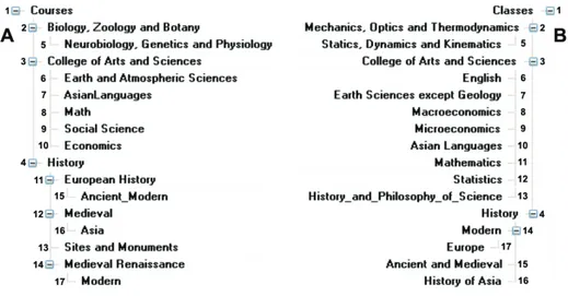
Let us summarize the algorithm for semantic matching via a running example. We consider small academic courses classifications shown in Figure 1.
Fig. 1. Parts of two classifications devoted to academic courses
Let us introduce some notation (see also Figure 1). Numbers are the unique identi-fiers of nodes. We use “C” for concepts of labels and concepts at nodes. Thus, for
2 Notice idk is an explicit statement that the system is unable to compute any of the declared (four) relations. This should be interpreted as either there is not enough background knowledge, and therefore, the system cannot explicitly compute any of the declared relations or, indeed, none of those relations hold according to an application.
ample, in the tree A, CHistory and C4 are, respectively, the concept of the label History and the concept at node 4. Also, to simplify the presentation, whenever it is clear from the context we assume that the concept of a label can be represented by the label it-self. In this case, for example, CHistory becomes denoted as History. Finally, we some-times use subscripts to distinguish between trees in which the given concept of a label occurs. For instance, HistoryA, means that the concept of the label History belongs to the tree A.
The algorithm takes as input two schemas and computes as output a set of map-ping elements in four macro steps:
− Step 1: for all labels L in two trees, compute concepts of labels, CL. − Step 2: for all nodes N in two trees, compute concepts at nodes, CN. − Step 3: for all pairs of labels in two trees, compute relations among CL’s. − Step 4: for all pairs of nodes in two trees, compute relations among CN’s.
The first two steps represent the preprocessing phase, while the third and the fourth steps are the element level and structure level matching respectively3. It is im-portant to notice that Step 1 and Step 2 can be done once, independently of the spe-cific matching problem. Step 3 and Step 4 can only be done at run time, once the two trees which must be matched have been chosen. We also refer in the remainder of the paper to the element level matching (Step 3) as label matching and to the structure level matching (Step 4) as node matching.
We view labels of nodes as concise descriptions of the data that is stored under the nodes. During Step 1, we compute the meaning of a label at a node (in isolation) by taking as input a label, by analyzing its real-world semantics (e.g., using WordNet [37] 4), and by returning as output a concept of the label. Thus, for example, by writ-ing CHistory we move from the natural language ambiguous label History to the concept
CHistory, which codifies explicitly its intended meaning, namely the data (documents) which are about history.
During Step 2 we analyze the meaning of the positions that the labels of nodes have in a tree. By doing this we extend concepts of labels to concepts at nodes. This is required to capture the knowledge residing in the structure of a tree, namely the con-text in which the given concept of label occurs [17]. Thus, for example, in the tree A, when we write C4 we mean the concept describing all the documents of the (aca-demic) courses, which are about history.
Step 3 is concerned with acquisition of “world” knowledge. Relations between
concepts of labels are computed with the help of a library of element level semantic matchers. These matchers take as input two concepts of labels and produce as output a semantic relation (e.g., equivalence, more/less general) between them. For example, from WordNet [37] we can derive that course and class are synonyms, and therefore,
CCourses = CClasses.
3 Element level matching (techniques) compute mapping elements by analyzing schema entities in isolation, ignoring their relations with other entities. Structure-level techniques compute mapping elements by analyzing how schema entities appear together in a structure, see for more details [42,43].
4 WordNet is a lexical database for English. It is based on synsets (or senses), namely structures containing sets of terms with synonymous meanings.
Step 4 is concerned with the computation of the relations between concepts at
nodes. This problem cannot be resolved by exploiting static knowledge sources only. We have (from Step 3) background knowledge, codified as a set of relations between concepts of labels occurring in two trees. This knowledge constitutes the background theory (axioms) within which we reason. We need to find a semantic relation (e.g., equivalence, more/less general) between the concepts at any two nodes in two trees. However, these are usually complex concepts obtained by suitably combining the cor-responding concepts of labels. For example, suppose we want to find a relation be-tween C4 in the tree A (which, intuitively, stands for the concept of courses of history) and C4 in the tree B (which, intuitively, stands for the concept of classes of history). In this case, we should realize that they have the same extension, and therefore, that they are equivalent.
3. Step 1: Concepts of Labels Computation
Technically, the main goal of Step 1 is to automatically translate ambiguous natural language labels taken from the schema elements’ names into an internal logical lan-guage. We use a propositional description logic language5 (LC) for several reasons. First, given its set-theoretic interpretation, it “maps” naturally to the real world se-mantics. Second, natural language labels, e.g., in classifications, are usually short ex-pressions or phrases having simple structure. These phrases can often be converted into a formula in LC with no or little loss of meaning [18]. Third, a formula in LC can be converted into an equivalent formula in a propositional logic language with boo-lean semantics. Apart from the atomic propositions, the language LC includes logical operators, such as conjunction ( ), disjunction ( ), and negation (¬). There are also comparison operators, namely more general ( ), less general ( ), and equivalence (=). The interpretation of these operators is the standard set-theoretic interpretation.
We compute concepts of labels according to the following four logical phases, be-ing inspired by the work in [34].
1. Tokenization. Labels of nodes are parsed into tokens by a tokenizer which recog-nizes punctuation, cases, digits, stop characters, etc. Thus, for instance, the label
History and Philosophy of Science becomes 〈history, and, philosophy, of, science〉. The multiword concepts are then recognized. At the moment the list of all multi-word concepts in WordNet [37] is exploited here together with a heuristic which takes into account the natural language connectives, such as and, or, etc. For ex-ample, Earth and Atmospheric Sciences becomes 〈earth sciences, and,
atmos-pheric, sciences〉 since WordNet contains senses for earth sciences, but not for
at-mospheric sciences.
5 A propositional description logic language (LC) we use here is the description logic ALC lan-guage without the role constructor, see for more details [4]. Note, since we do not use roles, in practice we straightforwardly translate the natural language labels into propositional logic for-mulas.
2. Lemmatization. Tokens of labels are further lemmatized, namely they are morpho-logically analyzed in order to find all their possible basic forms. Thus, for instance,
sciences is associated with its singular form, science. Also here we discard from
further considerations some pre-defined meaningless (in the sense of being useful for matching) words, articles, numbers, and so on.
3. Building atomic concepts. WordNet is queried to obtain the senses of lemmas iden-tified during the previous phase. For example, the label Sciences has the only one token sciences, and one lemma science. From WordNet we find out that science has two senses as a noun.
4. Building complex concepts. When existing, all tokens that are prepositions, punc-tuation marks, conjunctions (or strings with similar roles) are translated into logical connectives and used to build complex concepts out of the atomic concepts con-structed in the previous phase. Thus, for instance, commas and conjunctions are translated into logical disjunctions, prepositions, such as of and in, are translated into logical conjunctions, and words like except, without are translated into nega-tions. Thus, for example, the concept of label History and Philosophy of Science is computed as CHistory and Philosophy of Science = (CHistory CPhilosophy) CScience, where
CScience = 〈science, {sensesWN#2}〉 is taken to be the union of two WordNet senses, and similarly for history and philosophy. Notice that natural language and is con-verted into logical disjunction, rather than into conjunction (see [34] for detailed discussion and justification for this choice).
The result of Step 1 is the logical formula for concept of label. It is computed as a full propositional formula were literals stand for atomic concepts of labels.
In Figure 2 we present the pseudo-code which provides an algorithmic account of how concepts of labels are built. In particular, the buildCLab function takes the tree of nodes context and constructs concepts of labels for each node in the tree. The nodes are preprocessed in the main loop in lines 220-350. Within this loop, first, the node label is obtained in line 240. Then, it is tokenized and lemmatized in lines 250 and 260, respectively. The (internal) loop on the lemmas of the node (lines 270-340) starts from stop words test in line 280. Then, WordNet is queried. If the lemma is in WordNet, its senses are extracted. In line 300, atomic concept of label is created and attached to the node by the addACOLtoNode function. In the case when Word-Net returns no senses for the lemma, the special identifier SENSES_NOT_FOUND is attached to the atomic concept of label6. The propositional formula for the concept of label is iteratively constructed by constructcLabFormula (line 340). Finally, the logical formula is attached to the concept at label (line 350) and some sense filter-ing is performed by elementLevelSenseFilterfilter-ing7.
6 This identifier is further used by element level semantic matchers in Step 3 of the matching algorithm in order to determine the fact that the label (lemma) under consideration is not con-tained in WordNet, and therefore, there are no senses in WordNet for a given concept.
7 The sense filtering problem is also known under the name of word sense disambiguation (WSD), see, e.g., [29].
Node struct of int nodeId; String label; String cLabel; String cNode; AtomicConceptAtLabel[] ACOLs; AtomicConceptOfLabel struct of int id; String token; String[] wnSenses;
200. void buildCLab(Tree of Nodes context) 210. String[] wnSenses;
220. For each node in context 230. String cLabFormula=””;
240. String nodeLabel=getLabel(node); 250. String[] tokens=tokenize(nodeLabel); 260. String[] lemmas=lematize(tokens); 270. For each lemma in lemmas
280. if (isMeaningful(lemma)) 290. if (!isInWordnet(lemma))
300. addACOLtoNode(node, lemma, SENSES_NOT_FOUND); 310. else
320. wnSenses= getWNSenses(token);
330. addACOLtoNode(node, lemma, wnSenses);
340. cLabFormula=constructcLabFormula(cLabFormula, lemma); 350. setcLabFormula(node, cLabFormula);
360. elementLevelSenseFiltering(node); Fig. 2. Concept of label construction pseudo code
The pseudo code in Figure 3 illustrates the sense filtering technique. It is used in order to filter out the irrelevant (for the given matching task) senses from concepts of labels. In particular, we look whether the senses of atomic concepts of labels within each concept of a label are connected by any relation in WordNet. If so, we discard all other senses from atomic concept of label. Otherwise we keep all the senses. For ex-ample, for the concept of label Sites and Monuments before the sense filtering step we have 〈Sites, {sensesWN#4}〉 〈Monuments, {sensesWN#3}〉. Since the second sense of
monument is a hyponym of the first sense of site, notationally Monument#2 Site#1,
all the other senses are discarded. Therefore, as a result of this sense filtering step we have 〈Sites, {sensesWN#1}〉 〈Monuments, {sensesWN#1}〉.
elementLevelSenseFiltering takes the node structure as input and dis-cards the irrelevant senses from atomic concepts of labels within the node. In particu-lar, it executes two loops on atomic concept of labels (lines 30-120 and 50-120). WordNet senses for the concepts are acquired in lines 40 and 70. Then two loops on the WordNet senses are executed in lines 80-120 and 90-120. Afterwards, checking whether the senses are connected by a WordNet relation is performed in line 100. If so, the senses are added to a special set, called refined senses set (lines 110, 120). Fi-nally, the WordNet senses are replaced with the refined senses by saveRefined-Senses.
10.void elementLevelSenseFiltering(Node node)
20. AtomicConceptOfLabel[] nodeACOLs=getACOLs(node); 30. for each nodeACOL in nodeACOLs
40. String[] nodeWNSenses=getWNSenses(nodeACOL); 50. for each ACOL in nodeACOLs
60. if (ACOL!=nodeACOL)
70. String[] wnSenses=getWNSenses(ACOL); 80. for each nodeWNSense in nodeWNSenses 90. for each wnSense in wnSenses
100. if (isConnectedbyWN(nodeWNSense, focusNodeWNSense)) 110. addToRefinedSenses(nodeACOL,nodeWNSense);
120. addToRefinedSenses(focusNodeACOL, focusNodeWNSense); 130. saveRefinedSenses(context);
140. void saveRefinedSenses(context) 150. for each node in context
160. AtomicConceptOfLabel[] nodeACOLs=getACOLs(node); 170. for each nodeACOL in NodeACOLs
180. if (hasRefinedSenses(nodeACOL))
190. //replace original senses with refined Fig. 3. The pseudo code of element level sense filtering technique
4. Step 2: Concepts at Nodes Computation
Concepts at nodes are written in the same propositional description logic language as concepts of labels. Classifications and XML schemas are hierarchical structures where the path from the root to a node uniquely identifies that node (and also its meaning). Thus, following an access criterion semantics [26], the logical formula for a concept at node is defined as a conjunction of concepts of labels located in the path from the given node to the root. For example, in the tree A, the concept at node four is computed as follows: C4 = CCourses CHistory.
Further in the paper we require the concepts at nodes to be consistent (satisfiable). The reasons for their inconsistency are negations in atomic concepts of labels. For ex-ample, natural language label except_geology is translated into the following logical formula Cexcept_geology =¬Cgeology. Therefore, there can be a concept at node represented by a formula of the following type Cgeology … ¬ Cgeology,which is inconsistent. In this case the user is notified that the concept at node formula is unsatisfiable and asked to decide a more important branch, i.e., (s)he can choose what to delete from the tree, namely Cgeology or Cexcept_geology. Notice that this does not sacrifice the system performance since this check is made within the preprocessing (i.e., off-line, when the tree is edited)8. Let us consider the following example: C
N = … CMedieval CModern. Here, concept at node formula contains two concepts of labels, which are as from
8 In general case the reasoning is as costly as in the case of propositional logic (i.e., deciding unsatisfiability of the concept is co-NP hard). In many real world cases (see [25] for more de-tails) the corresponding formula is Horn. Thus, its satisfiability can be decided in linear time.
WordNet disjoint. Intuitively, this means that the context talks about either Medieval or Modern (or there is implicit disjunction in the concept at node formula). Therefore, in such cases, the formula for concept at node is rewritten in the following way:
CN =(CMedieval CModern) ...
The pseudo code of the second step is presented in Figure 4. The buildCNode function takes as an input the tree of nodes with precomputed concepts of labels and computes as output the concept at node for each node in the tree. The sense filtering (line 620) is performed by structureLevelSenseFiltering in the way simi-lar to the sense filtering approach used at the element level (as discussed in Figure 3). Then, the formula for the concept at node is constructed within buildcNodeFor-mula as conjunction of concepts of labels attached to the nodes in the path to the root. Finally, the formula is checked for unsatisfiability (line 640). If so, user is asked about the possible modifications in the tree structure or they are applied automati-cally, specifically implicit disjunctions are added between disjoint concepts (line 650).
600. void buildCNode(Tree of Node context) 610. for each node in context
620. structureLevelSenseFiltering (node,context);
630. String cNodeFormula= buildcNodeFormula (node, context); 640. if (isUnsatisifiable(cNodeFormula))
650. updateFormula(cNodeFormula); Fig. 4. Concepts at nodes construction pseudo code
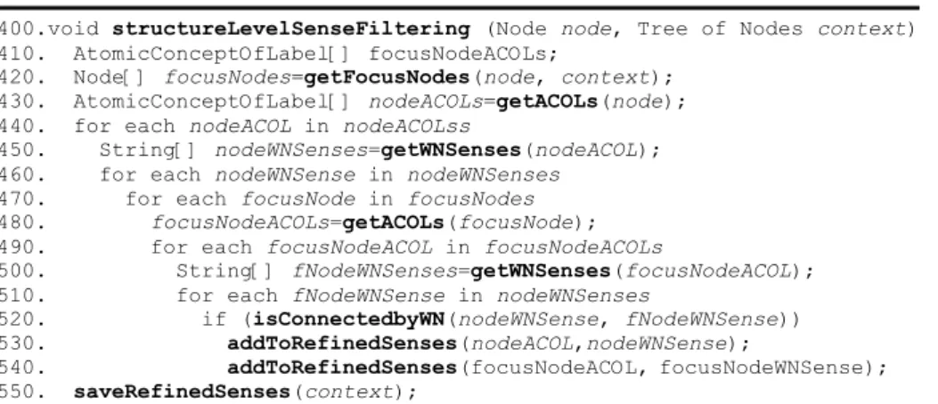
Let us discuss how the structure level sense filtering operates. As noticed before, this technique is similar to the one described in Figure 3. The major difference is that the senses now are filtered not within the node label but within the tree structure. For all concepts of labels we collect all their ancestors and descendants. We call them a
focus set. Then, all WordNet senses of atomic concepts of labels from the focus set
are compared with the senses of the atomic concepts of labels of the concept. If a sense of atomic concept of label is connected by a WordNet relation with the sense taken from the focus set, then all other senses of these atomic concepts of labels are discarded. Therefore, as a result of sense filtering step we have (i) the WordNet senses which are connected with any other WordNet senses in the focus set or (ii) all the WordNet senses otherwise. After this step the meaning of concept of labels is rec-onciled with respect to the knowledge residing in the tree structure. The pseudo code in Figure 5 provides an algorithmic account of the structure level sense filtering pro-cedure.
The structureLevelSenseFiltering function takes a node and a tree of nodes as input and refines the WordNet senses within atomic concepts of labels in the node with respect to the tree structure. First, atomic concepts at labels from the ances-tor and descendant nodes are gathered into the focus set (line 420). Then, a search for pairwise relations between the senses attached to the atomic concepts of labels is per-formed (lines 440-520). These senses are added to the refined senses set (lines 530-540) and further saveRefinedSenses from Figure 3 is applied (line 550) in order to save the refined senses.
400.void structureLevelSenseFiltering (Node node, Tree of Nodes context) 410. AtomicConceptOfLabel[] focusNodeACOLs;
420. Node[] focusNodes=getFocusNodes(node, context); 430. AtomicConceptOfLabel[] nodeACOLs=getACOLs(node); 440. for each nodeACOL in nodeACOLss
450. String[] nodeWNSenses=getWNSenses(nodeACOL); 460. for each nodeWNSense in nodeWNSenses
470. for each focusNode in focusNodes 480. focusNodeACOLs=getACOLs(focusNode); 490. for each focusNodeACOL in focusNodeACOLs
500. String[] fNodeWNSenses=getWNSenses(focusNodeACOL); 510. for each fNodeWNSense in nodeWNSenses
520. if (isConnectedbyWN(nodeWNSense, fNodeWNSense)) 530. addToRefinedSenses(nodeACOL,nodeWNSense);
540. addToRefinedSenses(focusNodeACOL, focusNodeWNSense); 550. saveRefinedSenses(context);
Fig. 5. The pseudo code of structure level sense filtering technique
5. Step 3: Label Matching
5.1 A library of label matchers
Relations between concepts of labels are computed with the help of a library of ele-ment level semantic matchers [24]. These matchers take as input two atomic concepts of labels and produce as output a semantic relation between them. Some of them are re-implementations of well-known matchers used in Cupid [32] and COMA [11]. The most important difference is that our matchers ultimately return a semantic relation, rather than an affinity level in the [0,1] range, although sometimes using customizable thresholds.
Our label matchers are briefly summarized in Table 1. The first column contains the names of the matchers. The second column lists the order in which they are exe-cuted. The third column introduces the matchers’ approximation level. The relations produced by a matcher with the first approximation level are always correct. For ex-ample, name brand as returned by WordNet. In fact, according to WordNet name is a hypernym (superordinate word) of brand. Notice that name has 15 senses and brand has 9 senses in WordNet. We use sense filtering techniques to discard the irrelevant senses, see Sections 3 and 4 for details. The relations produced by a matcher with the second approximation level are likely to be correct (e.g., net = network, but hot =
ho-tel by Prefix). The relations produced by a matcher with the third approximation level
depend heavily on the context of the matching task (e.g., cat = dog by Extended gloss
comparison in the sense that they are both pets). Note, matchers by default are
exe-cuted following the order of increasing approximation level. The fourth column re-ports the matchers’ type. The fifth column describes the matchers’ input.
Table 1. Element level semantic matchers implemented so far.
Matcher name ExecutionOrder Approximation level Matcher type Schema info
Prefix 2 2 Suffix 3 2 Edit distance 4 2 N-gram 5 2 Labels Text Corpus 13 3 String-based Labels + Corpus WordNet 1 1
Hierarchy distance 6 3 Sense-based WordNet senses
WordNet Gloss 7 3
Extended WordNet Gloss 8 3
Gloss Comparison 9 3
Extended Gloss Comparison 10 3
Semantic Gloss Comparison 11 3
Extended semantic gloss
com-parison 12 3
Gloss-based WordNet senses
We have three main categories of matchers: string-, sense- and gloss- based matchers. String-based matchers exploit string comparison techniques in order to pro-duce the semantic relation, while sense-based exploit the structural properties of the WordNet hierarchies and gloss-based compare two textual descriptions (glosses) of WordNet senses. Below, we discuss in detail some matchers from each of these cate-gories.
5.1.1 Sense-based matchers
We have two sense-based matchers. Let us discuss how the WordNet matcher works. As it was already mentioned, WordNet [37] is based on synsets (or senses), namely structures containing sets of terms with synonymous meanings. For example, the words night, nighttime and dark constitute a single synset. Synsets are connected to one another through explicit (lexical) semantic relations. Some of these relations (hy-pernymy, hyponymy for nouns and hypernymy and troponymy for verbs) constitute
kind-of and part-of (holonymy and meronymy for nouns) hierarchies. For instance, tree is a kind of plant. Thus, tree is hyponym of plant and plant is hypernym of tree.
Analogously, from trunk being a part of tree we have that trunk is meronym of tree and tree is holonym of trunk.
The WordNet matcher translates the relations provided by WordNet to semantic re-lations according to the following rules:
- A B, if A is a hyponym, meronym or troponym of B; - A B, if A is a hypernym or holonym of B;
- A = B, if they are connected by synonymy relation or they belong to one synset (night and nighttime from the example above);
- A ⊥ B, if they are connected by antonymy relation or they are the siblings in the
part of hierarchy.
5.1.2 String-based matchers
We have five string-based matchers. Let us discuss how the Edit distance matcher works. It calculates the number of simple editing operations (delete, insert and
re-place) over the label’s characters needed to transform one string into another, normal-ized by the length of the longest string. The result is a value in [0,1]. If the value ex-ceeds a given threshold (0.6 by default) the equivalence relation is returned, other-wise, Idk is produced.
5.1.3 Gloss-based matchers
We have six gloss-based matchers. Let us discuss how the Gloss comparison matcher works. The basic idea behind this matcher is that the number of the same words oc-curring in the two WordNet glosses increases the similarity value. The equivalence re-lation is returned if the number of shared words exceeds a given threshold (e.g., 3).
Idk is produced otherwise. For example, suppose we want to match Afghan hound and Maltese dog using the gloss comparison strategy. Notice, although these two concepts
are breeds of dog, WordNet does not have a direct lexical relation between them, thus the WordNet matcher would fail in this case. However, the glosses of both concepts are very similar. Maltese dog is defined as a breed of toy dogs having a long straight silky white coat. Afghan hound is defined as a tall graceful breed of hound with a long silky coat; native to the Near East. There are 4 shared words in both glosses, namely breed, long, silky, coat. Hence, the two concepts are taken to be equivalent.
5.2 The label matching algorithm
The pseudo code implementing Step 3 is presented in Figure 6. The label matching algorithm produces (with the help of matchers of Table 1) a matrix of relations be-tween all the pairs of atomic concepts of labels from both trees.
700. String[][] fillCLabMatrix(Tree of Nodes source,target); 710. String[][]cLabsMatrix;
720. String[] matchers; 730. int i,j;
740. matchers=getMatchers();
750. for each sourceAtomicConceptOfLabel in source 760. i=getACoLID(sourceAtomicConceptOfLabel); 770. for each targetAtomicConceptOfLabel in target 780. j= getACoLID(targetAtomicConceptOfLabel); 790. cLabsMatrix[i][j]=getRelation(matchers,
sourceAtomicConceptOfLabel,targetAtomicConceptOfLabel);
795. return cLabsMatrix
800. String getRelation(String[] matchers,
AtomicConceptOfLabel source, target)
810. String matcher; 820. String relation=”Idk”; 830. int i=0; 840. while ((i<sizeof(matchers))&&(relation==”Idk”)) 850. matcher= matchers[i]; 860. relation=executeMatcher(matcher,source,target); 870. i++; 880. return relation; Fig. 6. Label matching pseudo code
fillCLabMatrix takes as input two trees of nodes. It produces as output the matrix of semantic relations holding between the atomic concepts of labels in both trees. First, the element level matchers of Table 1, which are to be executed (based on the configuration settings), are acquired in line 740. Then, for each pair of atomic concepts of labels in both trees, semantic relations holding between them are deter-mined by using the getRelation function (line 790).
getRelation takes as input an array of matchers and two atomic concepts of labels. It returns the semantic relation holding between this pair of atomic concepts of labels according to the element level matchers. These label matchers are executed (line 860) until the semantic relation different from Idk is produced. Notice that exe-cution order is defined by the matchers array.
The result of Step 3 is a matrix of the relations holding between atomic concepts of labels. A part of this matrix for the example in Figure 1 is shown in Table 2.
Table 2. cLabsMatrix: matrix of relations among the atomic concepts of labels.
Classes History Modern Europe
Courses = idk idk idk
History idk = idk idk
Medieval idk idk ⊥ idk
Asia idk idk idk ⊥
6. Step 4: Node Matching
During this step, we initially reformulate the tree matching problem into a set of node matching problems (one problem for each pair of nodes). Finally, we translate each node matching problem into a propositional validity problem. Let us first discuss in detail the tree matching algorithm. Then, we consider the node matching algorithm. 6.1 The tree matching algorithm
The tree matching algorithm is concerned with decomposition of the tree matching task into a set of node matching tasks. It takes as input two preprocessed trees ob-tained as a result of Steps 1,2 and a matrix of semantic relations holding between the atomic concepts of labels in both trees obtained as a result of Step 3. It produces as output the matrix of semantic relations holding between concepts at nodes in both trees. The pseudo code in Figure 7 illustrates the tree matching algorithm.
900.String[][] treeMatch(Tree of Nodes source, target, String[][]
cLabsMatrix)
910. Node sourceNode,targetNode; 920. String[][]cNodesMatrix, relMatrix; 930. String axioms, contextA, contextB; 940. int i,j;
960. For each sourceNode in source 970. i=getNodeId(sourceNode);
980. contextA=getCnodeFormula (sourceNode);
990. For each targetNode in target 1000. j=getNodeId(targetNode);
1010. contextB=getCnodeFormula (targetNode);
1020. relMatrix=extractRelMatrix(cLabsMatrix, sourceNode,
targetNode);
1030. axioms=mkAxioms(relMatrix);
1040. cNodesMatrix[i][j]=nodeMatch(axioms,contextA,contextB);
1050. return cNodesMatrix;
Fig. 7. The pseudo code of the tree matching algorithm
treeMatch takes two trees of Nodes (source and target) and the matrix of relations holding between atomic concepts of labels (cLabsMatrix) as input. It starts from two loops over all the nodes of source and target trees in lines 960-1040 and 990-1040. The node matching problems are constructed within these loops. For each node matching problem we take a pair of propositional formulas encoding con-cepts at nodes and relevant relations holding between the atomic concon-cepts of labels using the getCnodeFormula and extractRelMatrix functions respectively. The former are memorized as contextAand contextBin lines 980 and 1010. The latter are memorized in relMatrix in line 1020. In order to reason about relations between concepts at nodes, we build the premises (axioms) in line 1030. These are a conjunction of the concepts of labels which are related in relMatrix. For example, the semantic relations in Table 2, which are considered when we match C4 in the tree A and C4 in the tree B are ClassesB= CoursesA and HistoryB = HistoryA. In this case
axioms is (ClassesB↔ CoursesA)∧(HistoryB ↔ HistoryA). Finally, in line 1040, the semantic relations holding between the concepts at nodes are calculated by node-Match and are reported as a bidimensional array (cNodesMatrix). A part of this matrix for the example in Figure 1 is shown in Table 3.
Table 3. cNodesMatrix: matrix of relations among the concepts at nodes (match-ing result). C1 C4 C14 C17 C1 = C4 = C12 ⊥ ⊥ C16 ⊥ ⊥ A B
6.2 The node matching algorithm
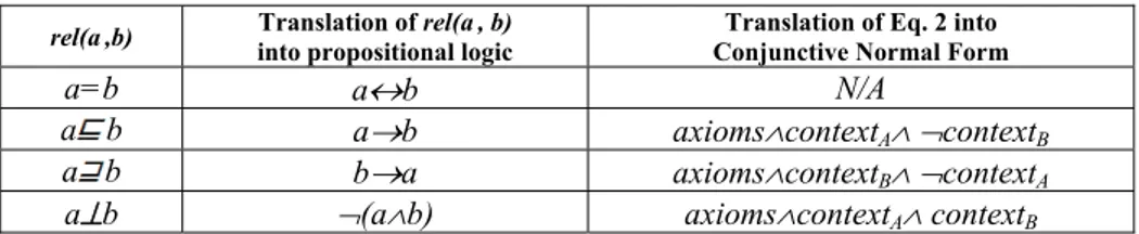
Each node matching problem is converted into a propositional validity problem. Se-mantic relations are translated into propositional connectives using the rules described in Table 4 (second column).
Table 4. The relationship between semantic relations and propositional formulas. rel(a,b) into propositional logic Translation of rel(a, b) Conjunctive Normal Form Translation of Eq. 2 into
a=b a↔b N/A
a b a→b axioms∧contextA∧ ¬contextB
a b b→a axioms∧contextB∧ ¬contextA
a⊥b ¬(a∧b) axioms∧contextA∧ contextB The criterion for determining whether a relation holds between concepts of nodes is the fact that it is entailed by the premises. Thus, we have to prove that the following formula:
(axioms) → rel(contextA , contextB ), (1) is valid, namely that it is true for all the truth assignments of all the propositional variables occurring in it. axioms, contextA, and contextB are as defined in the tree matching algorithm. rel is the semantic relation that we want to prove holding be-tween contextA and contextB. The algorithm checks the validity of Eq. 1 by proving that its negation, i.e., Eq. 2, is unsatisfiable.
axioms ∧¬ rel(contextA , contextB ) (2) Table 4 (third column) describes how Eq. 2 is translated before testing each seman-tic relation. Noseman-tice that Eq. 2 is in Conjunctive Normal Form (CNF), namely it is a conjunction of disjunctions of atomic formulas. The check for equivalence is omitted in Table 4, since A=B holds if and only if A B and A B hold, i.e., both
axi-oms∧contextA∧¬contextB and axioms∧contextB∧¬contextA are unsatisfiable formulas. We assume the labels of nodes and the knowledge derived from element level se-mantic matchers to be all globally consistent. Under this assumption the only reason why we get an unsatisfiable formula is because we have found a match between two nodes. In fact, axioms cannot be inconsistent by construction. Consistency of contextA and contextB is checked in the preprocessing phase (see, Section 4 for details). How-ever, axioms and contexts (for example, axioms∧contextA) can be mutually inconsis-tent. The situation occurs, for example, when axioms entails negation of the variable occurring in the context. In this case, the concepts at nodes are disjoint. In order to guarantee the correct behavior of the algorithm we perform the disjointness test first. It does not influence the algorithm correctness in general but allow us to obtain the correct result in this special case.
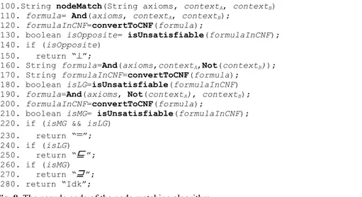
Let us consider the pseudo code of a basic node matching algorithm, see Figure 8. In line 1110, nodeMatch constructs the formula for testing disjointness. In line 1120, it converts the formula into CNF, while in line 1130 it checks the CNF formula for unsatisfiability. If the formula is unsatisfiable the disjointness relation is returned.
Then, the process is repeated for the less and more general relations. If both rela-tions hold, then the equivalence relation is returned (line 1220). If all the tests fail, the
idk relation is returned (line 1280). In order to check the unsatisfiability of a
proposi-tional formula in a basic version of our NodeMatch algorithm we use the standard DPLL-based SAT solver [31].
1100.String nodeMatch(String axioms, contextA, contextB)
1110. formula= And(axioms, contextA, contextB);
1120. formulaInCNF=convertToCNF(formula);
1130. boolean isOpposite= isUnsatisfiable(formulaInCNF); 1140. if (isOpposite)
1150. return “⊥”;
1160. String formula=And(axioms,contextA,Not(contextB));
1170. String formulaInCNF=convertToCNF(formula); 1180. boolean isLG=isUnsatisfiable(formulaInCNF) 1190. formula=And(axioms, Not(contextA), contextB);
1200. formulaInCNF=convertToCNF(formula);
1210. boolean isMG= isUnsatisfiable(formulaInCNF); 1220. if (isMG && isLG)
1230. return “=”; 1240. if (isLG) 1250. return “ ”; 1260. if (isMG) 1270. return “ ”; 1280. return “Idk”;
Fig. 8. The pseudo code of the node matching algorithm
From the example in Figure 1, trying to prove that C4 in the tree B is less general than C4 in the tree A, requires constructing the following formula:
((ClassesB↔ CoursesA)∧(HistoryB↔ HistoryA)) ∧
(ClassesB∧HistoryB) ∧¬ (CoursesA∧HistoryA)
The above formula turns out to be unsatisfiable, and therefore, the less general re-lation holds. Notice, if we test for the more general rere-lation between the same pair of concepts at nodes, the corresponding formula would be also unsatisfiable. Thus, the final relation retuned by the NodeMatch algorithm for the given pair of concepts at nodes is the equivalence.
7. Semantic Matching with Attributes
So far we have focused on classifications, which are simple class hierarchies. If we deal with, e.g., XML schemas, their elements may have attributes, see Figure 9.
Attributes are 〈attribute−name, type〉 pairs associated with elements. Names for the attributes are usually chosen such that they describe the roles played by the do-mains in order to ease distinguishing between their different uses. For example, in the tree A, the attributes PID and Name are defined on the same domain string, but their intended use are the internal (unique) product identification and representation of the official products’ names, respectively. There are no strict rules telling us when data should be represented as elements, or as attributes, and obviously there is always more than one way to encode the same data. For example, in the tree A, PIDs are en-coded as strings, while in the tree B, IDs are enen-coded as ints. However, both attributes serve for the same purpose of the unique products’ identification. These observations suggest two possible ways to perform semantic matching with attributes: (i) taking into account datatypes, and (ii) ignoring datatypes.
The semantic matching approach is based on the idea of matching concepts, not their direct physical implementations, such as elements or attributes. If names of at-tributes and elements are abstract entities, therefore, they allow for building arbitrary concepts out of them. Instead, datatypes, being concrete entities, are limited in this sense. Thus, a plausible way to match attributes using the semantic matching ap-proach is to discard the information about datatypes. In order to support this claim, let us consider both cases in turn.
7.1 Exploiting datatypes
In order to reason with datatypes we have created a datatype ontology, OD, specified in OWL [45]. It describes the most often used XML schema built-in datatypes and re-lations between them. The backbone taxonomy of OD is based on the following rule:
the is-a relationship holds between two datatypes if and only if their value spaces are related by set inclusion. Some examples of axioms of OD are: float double, int ⊥ string, anyURI string, and so on. Let us discuss how datatypes are plugged within the four macro steps of the algorithm.
Steps 1,2. Compute concepts of labels and nodes. In order to handle attributes, we
ex-tend propositional description logics with the quantification construct and datatypes. Thus, we compute concepts of labels and concepts at nodes as formulas in the de-scription logics ALC(D) language [38]. For example, in the tree A in Figure 9, C4, namely, the concept at node describing all the string data instances which are the names of electronic photography products is encoded as follows: ElectronicsA (PhotoA CamerasA) ∃NameA.string.
Step 3. Compute relations among concepts of labels. In this step we extend our library
of element level matchers by adding a Datatype matcher. It takes as input two datatypes, it queries OD and retrieves a semantic relation between them. For example, from axioms of OD, the Datatype matcher can learn that float double, and so on.
Step 4. Compute relations among concepts at nodes. In the case of attributes, the node
matching problem is translated into an ALC(D) formula, which is further checked for its unsatisfiability using sound and complete procedures. Notice that in this case we have to test for modal satisfiability, not propositional satisfiability. The system we use is Racer [27]. From the example in Figure 9, trying to prove that C7 in the tree B is less general than C6 in the tree A, requires constructing the following formula:
((ElectronicsA=ElectronicsB) (PhotoA=PhotoB)
(CamerasA=CamerasB) (PriceA=PriceB) (float double))
(ElectronicsB (CamerasB PhotoB) ∃PriceB.float) ¬
(ElectronicsA (PhotoA CamerasA) ∃PriceA.double)
It turns out that the above formula is unsatisfiable. Therefore, C7 in the tree B is less general than C6 in the tree A. However, this result is not what the user expects. In fact, both C6 in the tree A and C7 in the tree B describe prices of electronic products, which are photo cameras. The storage format of prices in A and B (i.e., double and
float respectively) is not an issue at this level of detail.
Thus, another semantic solution of taking into account datatypes would be to build abstractions out of the datatypes, e.g., float, double, decimal should be abstracted to type numeric, while token, name, normalizedString should be abstracted to type string, and so on. However, even such abstractions do not improve the situation, since we may have, for example, an ID of type numeric in the first schema, and a conceptually equivalent ID, but of type string, in the second schema. If we continue building such abstractions, we result in having that numeric is equivalent to string in the sense that they are both datatypes.
The last observation suggests that for the semantic matching approach to be cor-rect, we should assume that all the datatypes are equivalent. Technically, in order to implement this assumption, we should add corresponding axioms (e.g., float = double) to the premises of Eq. 1. On the one hand, with respect to the case of not considering datatypes (see, Section 7.2), such axioms do not affect the matching result from the quality viewpoint. On the other hand, datatypes make the matching problem computa-tionally more expensive by requiring to handle the quantification construct.
7.2 Ignoring datatypes
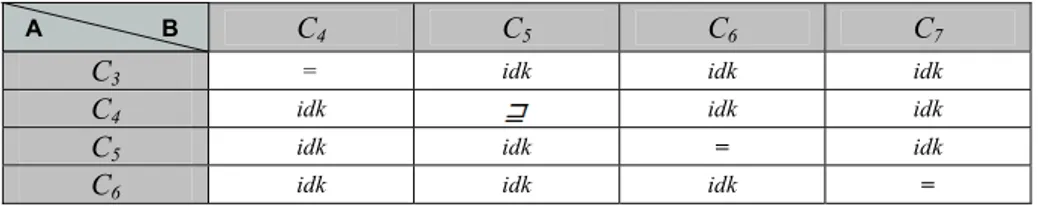
In this case, information about datatypes is discarded. For example, 〈Name, string〉 becomes Name. Then, the semantic matching algorithm builds concepts of labels out of attributes’ names in the same way as it does in the case of elements’ names, and so on. Finally, it computes mapping elements using the algorithm of Section 6. A part of the cNodesMatrix with relations holding between attributes for the example in Figure 9 is presented in Table 5. Notice that this solution allows a mappings’ computation not only between the attributes, but also between attributes and elements.
Table 5. Attributes: the matrix of semantic relations holding between concepts of nodes (the
matching result) for Figure 9.
C4 C5 C6 C7
C3 = idk idk idk
C4 idk idk idk
C5 idk idk = idk
C6 idk idk idk =
The task of determining mappings typically represents a first step towards the ulti-mate goal of, for example, data translation, query mediation, agent communication, and so on. Although information about datatypes will be necessary for accomplishing an ultimate goal, we do not discuss this issue any further since in this paper we con-centrate only on the mappings discovery task.
8. Efficient Semantic Matching
The node matching problem in semantic matching is a CO-NP hard problem, since it is reduced to the validity problem for the propositional calculus. In this section we present a set of optimizations for the node matching algorithm. In particular, we show that when dealing with conjunctive concepts at nodes, i.e., the concept at node is a conjunction (e.g., C7 in the tree A in Figure 1 is defined as AsianA LanguagesA), the node matching tasks can be solved in linear time. When we have disjunctive concepts
at nodes, i.e., the concept at node contains both conjunctions and disjunctions in any
order (e.g., C3 in the tree B in Figure 1 is defined as CollegeB (ArtsB SciencesB)), we use techniques allowing us to avoid the exponential space explosion which arises due to the conversion of disjunctive formulas into CNF. This modification is required since all state of the art SAT deciders take CNF formulas in input.
8.1 Conjunctive concepts at nodes
Let us make some observations with respect to Table 4 (Section 6.2). The first obser-vation is that the axioms part remains the same for all the tests, and it contains only clauses with two variables. In the worst case, it contains 2×nA×nB clauses, where nA and nB are the number of atomic concepts of labels occurred in contextA and contextB, respectively. The second observation is that the formulas for testing less and more general relations are very similar and they differ only in the negated context formula (e.g., in the test for less general relation contextB is negated). This means that Eq. 2 contains one clause with nB variables plus nA clauses with one variable. In the case of disjointness test contextA and contextB are not negated. Therefore, formula Eq. 2 con-tains nA + nB clauses with one variable.
8.1.1 The node matching problem by an example
Let us suppose that we want to match C16 in the tree A and C17 in the tree B in Figure 1. The relevant semantic relations between atomic concepts of labels are presented in Table 2. Thus, axioms is as follows:
(courseA↔classB)∧(historyA↔historyB) ∧
¬(medievalA∧modernB)∧ ¬(asiaA∧europeB) (3) which, when translated in CNF, becomes:
(¬courseA∨classB)∧( courseA∨¬classB)∧(¬ historyA∨historyB)∧
(historyA∨¬historyB) ∧ (¬medievalA∨¬modernB) ∧ (¬asiaA∨¬europeB) (4) As from Step 2, contextA and contextB are constructed by taking the conjunction of the concepts of labels in the path from the node under consideration to the root. Therefore, contextA and contextB are:
courseA∧historyA∧medievalA∧asiaA (5)
classB∧historyB∧modernB∧europeB (6) while their negations are:
¬courseA∨¬historyA∨¬medievalA∨¬asiaA (7) ¬classB∨¬historyB∨¬modernB∨¬europeB (8) So far we have concentrated on atomic concepts of labels. The propositional for-mulas remain structurally the same if we move to conjunctive concepts at labels. Let consider the following example:
Fig. 10. Two simple classifications (obtained by modifying, pruning the example in Figure 1)
Suppose we want to match C2 in the tree A and C2 in the tree B in Figure 10. Axi-oms required for this matching task are as follows: (courseA↔classB)∧
(historyA↔historyB)∧(medievalA⊥modernB)∧(asiaA⊥europeB). If we compare them with those of Eq. 3 and Eq.4, which represent axioms for the above considered exam-ple in Figure 1, we find out that they are the same. Furthermore, as from Step 2, the propositional formulas for contextA and contextB are the same for atomic and for con-junctive concepts of labels as long as they “globally” contain the same formulas. In fact, concepts at nodes are constructed by taking the conjunction of concepts at labels. Splitting a concept of a label with two conjuncts into two atomic concepts has no ef-fect on the resulting matching formula. The matching result for the matching tasks in Figure 10 is presented in Table 6.
Table 6. The matrix of relations between concepts at nodes (matching result) for Figure 10.
C1 C2
C1 =
C2 ⊥
8.1.2 Optimizations
Tests for less and more general relations. Using the observations in the beginning of Section 8.1 concerning Table 4, Eq. 2, with respect to the tests for less/more gen-eral relations, can be represented as follows:
(9) where n is the number of variables in contextA, m is the number of variables in
con-textB. The Ai’s belong to contextA, and the Bj’s belong to contextB. s, k, p are in the [0..n] range, while t, l, r are in the [0..m] range. q, w and v define the number of par-ticular clauses. Axioms can be empty. Eq. 9 is composed of clauses with one or two variables plus one clause with possibly more variables (the clause corresponding to the negated context). The key observation is that the formula in Eq. 9 is Horn, i.e., each clause contains at most one positive literal. Therefore, its satisfiability can be de-cided in linear time by the unit resolution rule [9]. Notice, that DPLL-based SAT solvers require quadratic time in this case [47].
In order to understand how the linear time algorithm works, let us prove the unsat-isfiability of Eq. 9 in the case of matching C16 in the tree A and C17 in the tree B in Figure 1. In this case, Eq. 9 is as follows:
(¬courseA∨classB)∧( courseA∨¬classB)∧(¬ historyA∨historyB)∧
(historyA∨¬historyB) ∧ (¬medievalA∨¬modernB)∧ (¬asiaA∨¬europeB)∧
courseA∧historyA∧medievalA∧asiaA∧
(¬classB∨¬historyB∨¬modernB∨¬europeB)
(10)
In Eq.10, the variables from contextA are written in bold face. First, we assign true to all unit clauses occurring in Eq. 10 positively. Notice these are all and only the clauses in contextA. This allows us to discard the clauses where contextA variables oc-cur positively (in this case: courseA∨¬classB, historyA∨¬historyB). The resulting for-mula is as follows:
classB∧historyB∧¬modernB∧¬europeB∧
(¬classB∨¬historyB∨¬modernB∨¬europeB) (11) Eq. 11 does not contain any variable derived from contextA. Notice that, by assign-ing true to classB, historyB and false to modernB, europeB we do not derive a contra-diction. Therefore, Eq. 10 is satisfiable. In fact, a (Horn) formula is unsatisfiable if and only if the empty clause is derived (and it is satisfiable otherwise).
Let us consider again Eq. 11. For this formula to be unsatisfiable, all the variables occurring in the negation of contextB (¬classB∨¬historyB∨¬modernB∨¬europeB in our example) should occur positively in the unit clauses obtained after resolving
axi-oms with the unit clauses in contextA (classB and historyB in our example). For this to happen, for any Bj in contextB there must be a clause of form ¬Ai∨Bj in axioms, where
we have the axioms of form A = Bj and Ai Bj. These considerations suggest the fol-lowing algorithm for testing satisfiability:
− Step 1. Create an array of size m. Each entry in the array stands for one Bj in Eq. 9. − Step 2. For each axiom of type Ai=Bj and Ai Bj mark the corresponding Bj. − Step 3. If all the Bj’s are marked, then the formula is unsatisfiable.
To complete the analysis, let us now suppose that we have not “europe”, but
“ex-cept europe” as a node of the tree depicted in Figure 1. This means that contextB con-tains the negated variable ¬europeB. Eq. 10 in this case is rewritten as follows:
(¬courseA∨classB)∧( courseA∨¬classB)∧(¬ historyA∨historyB)∧
(historyA∨¬historyB) ∧ (¬medievalA∨¬modernB)∧ (¬asiaA∨¬europeB)∧
courseA∧historyA∧medievalA∧asiaA∧
(¬classB∨¬historyB∨¬modernB∨europeB)
(12) Suppose that we have replaced all the occurrences of ¬europeB and europeB in the formula with europenB and ¬europenB respectively. In fact, we replace the variable with the new one which represents its negation. Notice that this replacement does not change the satisfiability properties of the formula. Truth assignment satisfying the new formula will satisfy the original formula after inverting the truth value of the new variable (europenB in our example). Notice also that the replacement changed the clause with europeB variable in axioms (¬asiaA∨europenB in Eq. 13).
(¬courseA∨classB)∧( courseA∨¬classB)∧(¬ historyA∨historyB)∧
(historyA∨¬historyB) ∧ (¬medievalA∨¬modernB)∧ (¬asiaA∨europenB)∧
courseA∧historyA∧medievalA∧asiaA∧
(¬classB∨¬historyB∨¬modernB∨¬europenB)
(13) Let us assign to true the unit clauses occurring in Eq. 13 positively. This allows us to discard a number of clauses. A simplified formula is depicted as Eq. 14.
classB∧historyB∧¬modernB∧europeB∧
(¬classB∨¬historyB∨¬modernB∨¬europenB) (14) This formula is satisfiable by assigning classB, historyB, europeB to true and
mod-ernB to false. Therefore, less general relation does not hold between the concept at node Asia and the concept at node Except Europe.
In order to construct an optimized algorithm for determining satisfiability of Eq. 13 let us compare Eq. 10 and Eq. 13. The parts of the formula representing contexts are the same. The differences are in axioms part of the formula and they are introduced by a variable replacement. Let us analyze how the replacement of the variable with its negations influences various classes of clauses in axioms, see Table 7.
Table 7. The correspondence between axioms and clauses.
Axioms Ai Bj
Ai=Bj
Bj Ai
Ai=Bj Ai⊥Bj
The classes of propositional clauses
With two variables ¬Ai∨Bj Ai∨¬Bj ¬Ai∨¬Bj The classes of clauses after replacement
of Ai with its negation Ani Ani∨Bj ¬Ani∨¬Bj Ani∨¬Bj The classes of clauses after replacement
of Bj with its negation Bnj ¬Ai∨¬Bnj Ai∨Bnj ¬Ai∨Bnj The classes of clauses after replacement of Ai and Bj
with their negations Ani and Bnj respectively Ani∨¬Bj ¬Ani∨Bj Ani∨Bj Let us concentrate on three classes of propositional clauses depicted in the second row of Table 7. As from Eq. 9, we have only these classes of clauses in axioms. The axioms from which the particular class of clauses can be derived are described in the first column. Rows 2-5 demonstrate how the replacement of variables with its nega-tion influences the clause. The first observanega-tion from Table 7 is that the new class of clauses (Ai∨Bj) is introduced in axioms. The variables derived from both contextA and
contextB occur in these clauses positively. This means that the clauses of form Ai∨Bj are discarded from the formula after unit propagation and cannot influence its satisfi-ability properties. The second observation is that all other clauses in Eq. 13 belong to the same classes as ones in Eq. 10. Therefore, the general observation made for Eq. 10 (namely, the formula is satisfiable if and only if there are clauses ¬Ai∨Bj in axioms for any Bj in contextB)holds for Eq. 13. As from Table 7, we have the clauses ¬Ai∨Bj in Eq. 13 in three cases:
− There are axioms Ai = Bj and Ai Bj, where Ai and Bj occur in contexts of the original formula positively.
− There are axioms Ai= Bj and Bj Ai, where Ai and Bj occur in contexts of the original formula negatively.
− There are axioms Ai⊥Bj, where Ai occurs in contextA of the original formula positively and Bj occurs in contextB of the original formula negatively.
These considerations suggest the following algorithm for testing the satisfiability (no-tice Step1 and Step 3 remain the same as in the previous version):
− Step 1. Create an array of size m. Each entry in the array stands for one Bj in Eq. 9. − Step 2a. If Ai and Bj occur positively in contextA and contextB respectively, for each
axiom Ai=Bj and Ai Bj mark the corresponding Bj.
− Step 2b. If Ai and Bj occur negatively in contextA and contextB respectively, for each axiom Ai=Bj and Bj Ai mark the corresponding Bj.
− Step 2c. If Bj occurs negatively in contextB and Ai occurs positively in contextA for each axiom Ai⊥Bj mark the corresponding Bj.
− Step 3. If all the Bj’s are marked, then the formula is unsatisfiable. The pseudo code of the optimized algorithm is presented in Figure 11.
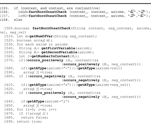
1155. if (contextA and contextB are conjunctive)
1156. isLG=fastHornUnsatCheck (contextA, contextB, axioms, “ ”,“ ”);
1157. isMG=fastHornUnsatCheck (contextB, contextA, axioms, “ ”,“ ”);
1158. else
1500.boolean fastHornUnsatCheck(String context, neg_context, axioms,
rel, neg_rel)
1510. int m=getNumOfVar(String neg_context); 1520. boolean array[m];
1530. for each axiom in axioms
1540. String Ai= getFirstVariable(axiom); 1550. String Bj= getSecondVariable(axiom); 1560. int j=getNumberInContext(Bj); 1570. if((occurs_positevely (Ai, context))&& (occurs_positevely (Bj, neg_context))) 1580. if((getAType(axiom)=”=”)||(getAType(axiom)=rel)) 1590. array[j]=true; 1600. if ((occurs_negatively (Ai, context))&& (occurs_negatively (Bj, neg_context))) 1610. if((getAType(axiom)=”=”)||(getAType(axiom)=neg_rel)) 1620. array[j]=true; 1630. if ((occurs_positevely (Ai, context))&& (occurs_negatively (Bj, neg_context))) 1640. if(getAType(axiom)=”⊥”) 1650. array[j]=true;
1660. for (i=0; i<m; i++) 1670. if (!array[i]) 1680. return false; 1690. return true;
Fig. 11. Optimization pseudo code of tests for less and more general relations
Thus, nodeMatch can be modified as in Figure 11 (the numbers on the left indi-cate where the new code must be positioned). fastHornUnsatCheck implements the three steps above. Step 1 is performed in lines (1510-1520). Then, a loop on
axi-oms (lines 1530-1650) implements Step 2. The final loop (lines 1660-1690)
imple-ments Step 3.
Disjointness test. Using the same notation as before in this section, Eq. 2 with respect to the disjointness test can be represented as follows:
(15) For example, the formula for testing disjointness between C16 in the tree A and C17 in the tree B in Figure 1 is as follows:
(¬courseA∨classB)∧( courseA∨¬classB)∧(¬ historyA∨historyB)∧
(historyA∨¬historyB) ∧ (¬medievalA∨¬modernB)∧ (¬asiaA∨¬europeB)∧
courseA∧historyA∧medievalA∧asiaA∧ classB∧historyB∧modernB∧europeB