U
NIVERSITÀ DEGLI
S
UDI DI
S
ALERNO
Facoltà di Scienze Matematiche Fisiche e Naturali
Dottorato di Ricerca in Fisica IX Ciclo II Serie
The neutrino interaction analysis chain in OPERA
Coordinatore del dottorato: Candidata:
Prof. Giuseppe Grella Dr.ssa Regina Rescigno
Relatori:
Prof. Giuseppe Grella
Università degli Studi di Salerno
Dr. Cristiano Bozza
Università degli Studi di Salerno
Correlatore: Prof. Dario Autiero
IPNL, Università Claude Bernard Lione I – Francia
Contents
Introduction ... i
Chapter 1... 1
1.1. Neutrino masses and mixing ...2
1.1.1. Mass generation ...2
1.1.2. Neutrino mixing...5
1.2. Neutrino oscillation...6
1.3. Neutrino oscillation experiments ...8
1.3.1. Solar neutrinos ...9
1.3.2. Atmospheric neutrinos ...11
1.3.3. Laboratory experiments ...15
1.4. The global oscillation picture ...21
Chapter 2... 23
2.1. The conceptual design of OPERA ...23
2.1.1. Experimental setup ...25
2.1.2. Operation mode...28
Contents _____________________________________ -ii-
2.2.1. Signal and background...30
2.2.2. Tau detection efficiency...33
2.2.3. Sensitivity to oscillations and discovery potential...34
Chapter 3... 36
3.1. Scanning system: hardware and software ...36
3.1.1. Nuclear emulsions...37
3.1.2. Particle track reconstruction...37
3.2. Vertex Location...41
3.2.1. CS scanning ...41
3.2.2. CS-Brick connection ...42
3.2.3. Scan-Back – Track Follow ...43
3.2.4. Volume Scan and Reconstruction ...45
3.3. Primary Vertex Study...46
3.3.1. The decay search procedure ...46
3.3.2. Scan-Forth and hadron interactions search...46
3.4. Sample results from the Salerno laboratory ...48
3.4.1. An example: Event #227200791 ...48
3.4.2. Location summary and performance ...50
3.4.3. General statistics ...52
3.5. OPERA status and performance ...55
Chapter 4... 58
4.1. Momentum measurement by MCS...58
4.1.1. Determination of the momentum with the official software...59
4.2. Review of the likelihood method ...60
4.3. The MCS in the likelihood approach ...61
4.3.1. The covariance matrix ...62
4.3.2. Implementation details...63
4.4. Summary of test results ...64
4.4.1. Simulated data ...64
4.4.2. Real data...68
Contents ____________________________________ -iii-
5.1. Definition of the “signal region” ...75
5.2. Results from simulations ...76
5.2.1. Estimation from experiment Proposal ...76
5.2.2. Estimation from FLUKA simulation...77
5.3. Cross–check with real data...81
5.3.1. Comparison with Scan-Forth data ...81
5.3.2. Comparison with pion test-beam...85
Chapter 6... 87
6.1. The primary vertex analysis...87
6.2. Monte-Carlo sample description...88
6.2.1. Sample with simulation of experimental resolutions ...88
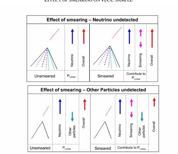
6.2.2. The effect of undetected particles...89
6.2.3. Photon recovery ...90
6.3. The missing transverse momentum ...93
6.3.1. Results from νμCC sample ...94
6.3.2. Results from νµNC and ντCC samples...99
6.4. The ϕ angle...106
6.5. Beyond the standard analysis chain ...109
6.5.1. The θ angle...109
6.5.2. The Qt variable...114
6.5.3. The a and g angles...115
6.6. Hadron re-interactions study...116
6.6.1. Integration of FLUKA simulation in the standard MC files ...117
6.6.2. Comparison of the results...117
Chapter 7... 124
7.1. Event topology...124
7.1.1. Event Tracks ...124
7.2. Kinematical analysis of the candidate event...126
7.2.1. The decay kinematics...127
7.2.2. The global kinematics ...128
Contents ____________________________________ -iv-
Conclusions ... 131
Appendix A ... 133
A.1. νμCC sample ...134
A.1.1. Non - smeared sample ...134
A.1.2. Smeared sample ...135
A.2. Comparison with νµCC sample...136
A.2.1. νμNC sample (neutrino as muon)...136
A.2.2. ντCC sample (tau as muon)...138
A.3. νµNC Sample ...140
A.3.1. Non - smeared sample ...140
A.3.2. Smeared sample ...141
A.4. ντCC Sample ...142
A.4.1. Non-smeared sample ...142
A.4.2 Smeared sample...143
References ...144
Introduction
The aim of the OPERA experiment is to provide a “smoking-gun” proof of neutrino oscillations, through the detection of the appearance signal of ντ’s in an initially pure νµ
beam. The beam is produced at CERN, 732 Km far from the detector, which is located underground in the Gran Sasso laboratory.
The evidence of the appearance signal will be provided by the detection of the daughter particles produced in the decay of the τ lepton. A micro-metric spatial resolution is needed in order to measure and study the topology of the ντ-induced events. With this
goal, nuclear emulsions, the highest resolution tracking detector, were chosen to be the core of the OPERA apparatus.
The analysis of the large amount of nuclear emulsions used in the OPERA experiment has required the development of a new generation of fast automatic microscopes, featuring a scanning speed more than one order of magnitude higher than in past emulsion-based experiments. The long R&D carried out by the Collaboration has given rise to two new systems: the European Scanning System (ESS) and the Japanese S-UTS. The work presented in this thesis has been carried out in one of the laboratories involved in the OPERA emulsion scanning, hosted at the University of Salerno, and during a 6 month’s stay at the IPNL (Institut de Physique Nucleaire de Lyon).
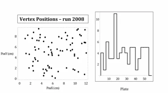
As for emulsion data-taking, several bricks from the 2008, 2009 and 2010 OPERA runs were scanned in Salerno and about 250 νµ-induced events were located. For the events
triggered in the 2008 run, a kinematical analysis was performed, by developing a new likelihood-based software, able to estimate the momentum of the particles traversing the emulsion sheets through multiple Coulomb scattering. The algorithm was also tested on a set of Monte-Carlo data and a set of pion tracks collected during the 2003, 2004 and 2007 test beam campaigns at CERN. The 2008 run sample was used also to perform the
Introduction _____________________________________ -ii-
hadron interaction search and the data collected were merged with those from other laboratories to estimate the background to the hadronic decay channel.
The kinematical analysis of the τØh decay channel is the subject of the second part of this thesis, developed while staying at the IPNL. The study on the quantities used to discriminate the signal and the background was accomplished by using simulated data. The kinematical cuts suggested by the OPERA Proposal were reviewed and the efficiencies obtained by applying these cuts were re-computed. In addition, another set of discriminating variables are suggested and their background suppression power is explored. Such estimators are proposed to be the subject of further work in the years to come.
Chapter 1
Neutrino Physics overview
In 1930 Wolfgang Pauli postulated the existence of the neutrino in order to reconcile data on the radioactive decay of nuclei with energy conservation [1]. In this decay neutrons are transformed into slightly lighter protons with emission of electrons:
neutron → proton + electron + antineutrino
Without neutrino, the energy conservation law required that electron and proton share the neutron energy. In this case each electron would be produced with a monochromatic energy distribution, whereas experiments observed a continuous spectrum, as would be expected for a three-body decay.
The postulated neutrino is chargless and interacts very weakly with matter; it just serves the purpose to balance energy and momentum in the above reaction. In fact, Pauli pointed out that for neutrino to do the job, it had to weigh less than one percent of proton mass, thus establishing the first limit of neutrino mass.
In the next years many efforts have been performed to confirm the existence of this new particle and to understand better its properties. Neutrinos were directly observed by Reines and Cowan in a nuclear reactor experiment in 1956 [2] and found to be left-handed in 1958 [3]. Four years later Lederman, Schwartz and Steinberger established that neutrinos associated to electrons and muons are different particles [4].
Since then, neutrinos have been considered as an essential part of the quantum description of fundamental particles and forces, the Standard Model of Particle Physics [5], [6], [7]. In absence of a direct observation of their masses, neutrinos are introduced in this model as fermionic massless particles.
Neutrino physics overview _____________________________________ -2-
The first clues that neutrino have mass came from a deep underground experiment carried out by Davis, detecting solar neutrinos. It revealed only about one-third of the flux predicted by Solar models [8], [9]. This result suggested that the solar neutrinos might be transforming into something else. Only electron neutrinos are emitted by the Sun and they could be converting to muon and tau neutrinos, not being detected by the experiments. This phenomen, called “neutrino oscillations”, was first proposed by Pontecorvo [10].
If neutrino oscillations exist, neutrinos have to be considered, in the Standard Model, as massive particles and their description needs to be revised.
In this chapter, an overview of Standard Model extensions is given and results of neutrino oscillation experiments are shown.
1.1.
Neutrino masses and mixing
The Standard Model of Particle Physics (SM) is a description of strong, weak and electromagnetic interactions. In the formulation provided by Glashow [5], Salam [7] and Weinberg [6], neutrinos are massless fermions having neither strong nor electromagnetic interactions. In the ‘basic’ SM, there are no RH (right-handed) neutrinos, according with the result of Goldhaber et al. [11] that weakly interacting neutrinos are always left-handed.
The non-existence of RH neutrinos is one of the reasons why neutrino mass might be vanishing. Unlike photons, no profound principle protect the neutrinos from having mass; therefore, by adding RH neutrinos, the Higgs mechanism of the Standard Model can give neutrinos the same type of mass as the electron mass or other charged lepton and quarks.
1.1.1.
Mass generation
In the Lagrangian density for the quantum field theory, the Dirac mass term can be written as:
( )
D D D R L L R
L =−m
ψψ
= −mψ ψ ψ ψ
+ 1.1Such Dirac mass term appears in this form but it can be regarded, for simplicity, as an ‘coupling’ between left-handed and right-handed particle fields (as shown in Figure 1.1). It is possible to add right-handed neutrinos (νR) to the Standard Model, providing that they do not take part in the weak interactions. A Dirac mass for the neutrino (mLR) would naturally arise as shown in the upper part of Figure 1.2. It is also possible to give neutrinos a new kind of mass called a Majorana1 [12] mass (mLL) if the LH neutrinos νL
Neutrino physics overview _____________________________________ -3-
are coupled with its own charge and parity conjugated state, the RH antineutrino (νLC ) where ‘C’ denotes the simultaneous operations of charge and parity conjugation.
RH neutrinos can also independently acquire their own Majorana masses MRR, by interacting with their own CP conjugates νRC (Figure 1.3).
In quantum field theory language, this is possible if new fields are added to the ‘basic’ Standard Model. An arbitrary number n of sterile neutrinos νs is added to the three standard generations and they can be used to construct two types of mass terms:
, , , ,
D M C
D s i ik L k M s i ij s j
L =
ν
Mν
L =ν
Mν
1.2where νL = (νL,1, νL,2, νL,3) are the three active neutrinos fields (only LH) and νs = (νs,1,
νs,2... νs,n) are RH sterile neutrino fields.
LD is the Dirac mass term and it is generated after spontaneous electroweak symmetry
breaking from a Yukawa-like interaction; it has a neutrino field and an antineutrino field, and conserves the total lepton number. MD is a complex 3 × n matrix.
LM is a Majorana mass term and since it involves two neutrino fields, it breaks lepton
number conservation by two units; MM is a symmetric matrix of dimension n × n.
The most general mass terms we can write for ν is a combination of Dirac and Majorana mass term:
(
)
. . C LL LR C L L s T LR RR s m m L h c m Mν
ν ν
ν
= − + 1.3To find the mass states we need to diagonalise the mass matrix, i.e. find its eigenvalues and eigenstates.
Figure 1.1: The electron Dirac mass me can be thought of as an interaction between a left-handed electron eL- and a right-handed electron eR-. The long (blue) arrows denote the electron momentum vector and the short (red) arrows denote the electron spin vector. For right-handed electrons eR-the spin vector and the momentum vector are aligned, whereas for left-handed electrons eL-they are opposite. The mass term may be regarded as interactions that enable left-handed electrons to interact with right -handed electrons.
Neutrino physics overview _____________________________________ -4-
Figure 1.2: For neutrinos there are two types of mass that are possible. As in the case of the electron there is the Dirac mass mLR,v that couples a left-handed neutrino vL to a right-handed neutrino vR (upper part of he diagram). The role of a right handed neutrino can be played by vLC obtained by transforming the left-handed neutrino vL under the operations charge and parity conjugation, where vLC is a right-handed neutrino. If vL interacts with vLC this results in Majorana mass term mLLv.
Figure 1.3: If right-handed neutrinos vR are added to the Standard Model, than they also acquire a Majorana mass term MRR by coupling to their own charge and parity conjugated states vRC.
1.1.1.a.The See-Saw Model
As anticipated in the previous section, three neutrino mass terms are possible. Majorana mass terms read mLLν νL LC and MRRν νR RC; the Dirac mass term reads mLRν νL R.
Although left-handed Majorana masses mLL are possible in principle, in the Standard
Model they are constrained to zero by the Higgs mechanism. However there is nothing preventing RH neutrinos from having Majorana masses MRR, where the magnitude of
such masses can take any value ; in particular such masses might be much larger than those of other particles. LH neutrinos take part in weak interactions with the W and Z bosons and if they were very heavy the theory would be disturbed. RH neutrinos on the other hand do not take part in weak interactions and so their mass MRR can be large. The
heaviness of MRR cannot be motivated in the framework of the Standard Model, but if
one believes that the Standard Model is a theory that describes the world only at low energies, it is quite natural to expect that the mass MRR is generated at ultra-high energy
by the symmetry breaking of the theory beyond the Standard Model.
The idea of the simplest version of See-Saw mechanism [13], [14] is to assume that the mass terms mLL are zero to begin with, but are generated effectively, after RH neutrinos
are introduced. Another fundamental assumption, as anticipated, is that MRR >> mLR. In
Neutrino physics overview _____________________________________ -5-
(
)
0 . . C LR C L L s T LR RR s m L h c m Mν
ν ν
ν
= − + 1.4In the approximation that MRR >> mLR the matrix can be diagonalised to yield effective
Majorana masses of the type mLL:
1 T
LL LR RR LR
m =m M− m
The effective left-handed Majorana masses mLL are naturally suppressed by the heavy
scale MRR.
1.1.2.
Neutrino mixing
Two different neutrino bases have been introduced, (νe, νµ, ντ) being the flavour basis,
and (ν1, ν2, ν3) being the neutrino mass basis.
The three flavour states are related to the three neutrino mass states by an unitary matrix U, the “lepton mixing matrix” (known as the Pontecorvo-Maki-Nakagawa-Sakata matrix [15], [16]): 1 2 3 1 1 2 3 2 1 2 3 3 e Ue Ue Ue U U U U U U µ µ µ µ τ τ τ τ
ν
ν
ν
ν
ν
ν
= 1.5This 3×3 matrix can be parameterized in terms of three mixing angles θij and three complex phases (one named after Dirac and the other two after Majorana). Generally, a unitary matrix has six phases but, in this case, three of them are removed by properly choosing the eigenstates. Since the neutrino masses are Majorana there is no additional phase associated with them.
The most common parameterization of the mixing matrix is:
1 2 / 2 13 13 12 12 / 2 23 23 12 12 23 23 13 13 1 0 0 0 0 0 0 0 0 1 0 0 0 0 0 0 0 0 1 0 0 1 i i i i c s e c s e U c s s c e s c s e c α δ α δ − − = − − − 1.6
where sij and cij stand for, respectively, the sines and cosines of the mixing angles θij, δ is the Dirac phase and αi (i = 1, 2) are the Majorana phases.
The matrix U is factorized in a matrix product of four matrices associated with the physics of neutrinos coming from different sources. As will be shown in section 1.3,
Neutrino physics overview _____________________________________ -6-
experiments with three different neutrino sources are possible and they investigate different oscillation channels.
Atmospheric neutrinos experiments suggest the possibility of having νµ → ντ oscillation
(first matrix). The second matrix is associated with the physics of reactor neutrino oscillations (νe → νµ,ντ) and here a δ phase (providing a possible source of CP violation) appears [17], [18], [19]. The third matrix is probed by experiments with Solar neutrinos (commonly interpreted as νe → νµ oscillations). The last matrix contains the Majorana
phases that are not involved in neutrino oscillations.
1.2.
Neutrino oscillation
The history of neutrino oscillations dates back to the work by Pontecorvo who in 1957 proposed ν →ν oscillations in analogy with K→K oscillations, described as the mixing of two Majorana neutrinos [16]. Pontecorvo was the first to realise that what we call “electron neutrino”, for example, may be a linear combination of mass eigenstate neutrinos, and that this feature could lead to neutrino oscillations such as νe → νµ.
Neutrino oscillations in vacuum would arise if neutrinos are massive ad mixed. From equation 1.5 we see that if neutrinos have mass, the eigenstate να (α = e, µ, τ) produced
in a weak interaction with energy E is, in general, a linear combination of the mass eigenestates νi with energy Ei, and mass mi
* 1 n i i i U α α ν ν = =
∑
1.7After travelling a distance L (or, equivalently, time t) a neutrino originally produced with a flavor α evolves as follows:
* 1 ( ) ( ) ( ) i (0) n iE t i i i i i t U t where t e α α ν ν ν − ν = =
∑
= 1.8The probability to find state |νβ> after a time t, starting from a state |να> is:
2 2 * 1 ( ) ( ) (0) i n iE t i i i P
ν
αν
βν
β tν
α U eβ − Uα = → = =∑
1.9Remembering that U is a unitary matrix and by using the ultra-relativistic approximations Ei = pi2+mi2 ≃ pi+mi / 2E it is possible to rewrite equation 1.9 as:
Neutrino physics overview _____________________________________ -7- 2 1 2 * 2 2 ( ) [ 1] i m n i L E i i i P
ν
αν
βδ
αβ U Uβ α e ∆ − = → = +∑
− 1.10where ∆mi21 =mi2−m12 and L = ct is the distance between the source and the detector. Equation (1.10) shows that transition probability depends on elements of the mixing matrix, on the difference of the squares of neutrino masses and on the parameter L/E,
defined by the experimental setup. If U = I and/or
2 1 1 i m L E ∆
≪ the neutrino oscillation
does not show up.
In the simplified scenario of two-neutrino mixing between να, νβ, there is only one
mass-squared difference and the mixing matrix can be parameterized in terms of one mixing angle: cos sin sin cos U
θ
θ
θ
θ
= − 1.11The resulting transition probability between different flavors can be written as:
2 2 2 ( ) sin 2 sin 4 m L P E α β
ν
→ν
=θ
∆ 1.12This expression can be also cast in the shape:
2 2 2 2 ( / )( / ) ( ) sin 2 sin 1.27 ( / ) m eV L Km P E GeV α β
ν
→ν
=θ
∆ 1.13This expression is useful because the results of oscillations experiments are often analysed in first approximation in a two-family scenario. An experiment is characterized by the typical neutrino energy E and by the source-detector distance L. Once these variables are fixed, different values of transition probability are possible, depending on ∆m2 and sin22
θ
. The constraints on P(να→νβ) are translated into allowedor excluded regions in the (∆m2, sin22
θ
) plane by inverting expression 1.13.In order to be sensitive to a given value of ∆m2 , an experiment can be optimised
choosing 2
/ ( osc)
E L≈ ∆m L∼L where Losc =E/∆m2. If (E/L) >> ∆m2 (L << Losc) the
oscillation does not have enough time to yield a detectable effect because sin2(∆m2L/E) << 1.
Neutrino physics overview _____________________________________ -8-
If (E/L) << ∆m2 (L >> Losc), it is possible to show that the oscillation phase goes through many cycles before the detection and it is smeared out to sin2(∆m2L/E) = 1/2 by
the finite spread of the energy spectrum and of the source-detector distance.
For null results that set an upper bound on the oscillation probability P(να→νβ) ≤ PL , the excluded region lies always on the upper right side of the (∆m2, sin22
θ
) plane, limited by the followed asymptotic lines (see Figure 1.4):• A vertical line at sin22
θ
= 2PL, for ∆m2 >> E/L (by setting sin2(∆m2L/E) = ½ on average)• For ∆m2 << E/L the oscillation phase can be replaced by its first-order expansion and the limiting curve takes the form
2
sin 2 4 L / ( / )
m
θ
P L E∆ =
A positive result, i.e. a non-vanishing fraction of oscillated neutrinos, can be used to define a confidence region on P(να→νβ), which translates to equal probability contours
on the (∆m2, sin22
θ
) plane.Figure 1.4: The characteristic form of an excluded region from a negative search with fixed L/E and of an allowed region from a positive search with varying L/E in the two-neutrino oscillation parameter plane
1.3.
Neutrino oscillation experiments
There are a large number of experiments trying to observe neutrino oscillations. Some rely on man-made sources like nuclear reactors or accelerators; others rely on “natural” sources such as solar neutrinos or neutrinos from cosmic-rays (atmospheric neutrinos).
Neutrino physics overview _____________________________________ -9-
All of these neutrino oscillation experiments are complementary because they involve neutrinos of different energies travelling over different distances.
The detectors are designed to be large in order to compensate the small neutrino interaction cross sections and are often placed underground to shield the cosmic muons. The accelerator experiments can be classified into short-baseline (SBL) and
long-baseline (LBL) depending on the source-detector distance. This quantity spans from a
few km (in SBL experiments) to hundreds of km (in LBL experiments).
1.3.1.
Solar neutrinos
Solar neutrinos are produced by the nuclear fusion process in the core of the Sun, which yields exclusively the electron flavor. These neutrinos are produced with different energies; this is reflected in the design of solar neutrino experiments, each of which probes a specific energy range (Figure 1.5).
The first result on detection of solar neutrinos was announced by Davis in 1968. In the gold mine of Homestake [20], [21] , the solar neutrinos flux was measured for about 30 years and found lower by about 1/3 with respect to predictions of the Standard Solar Model (SSM). The favoured explanation for this deficit is the neutrino oscillations. The solar neutrinos flux has been measured also by other experiments (GALLEX [22], [23], [24], Kamiokande [25], SuperKamiokande [26], [27] – see Table 1.1), all finding a deficit, but with disagreeing quantitative results. The most complete scenario comes from SNO (Sudbury Neutrino Observatory) in Canada. The experiment measured both the flux of electron neutrinos (CC interactions) [28] and the total flux of all three types of neutrinos (by NC interactions) [29], [30]. The SNO data shows that the SSM is correct, and the Solar neutrino deficit was a result of the oscillation of electron neutrinos into νµ and ντ, which were below the energy threshold to produce CC interactions. The
three-flavor oscillation picture also allows to reconcile the results of almost all experiments, by folding the neutrino production spectra with the L/E oscillation dependence. Neutrino oscillations consistent with solar neutrino observations have been seen using man-made neutrinos from nuclear reactors at KamLAND [31], [32] in Japan. KamLAND has already seen a signal of neutrino oscillations in the so-called Solar neutrino LMA (Large Mixing Angle) mass range.
By combining KamLAND and SNO results with other solar neutrino data (especially that of SuperKamiokande) it is possible to remove ambiguities and estimate two oscillation parameters: 2 0.18 12 0.15 sin 2θ =0.314(1+− ) 1.14 2 5 2 21 7.92(1 0.09) 10 m − eV ∆ = ± × 1.15
Neutrino physics overview ___________________________________ -10-
Figure 1.5: The predicted unoscillated spectrum dΦ/dE ν of solar neutrinos, together with the energy thresholds of the experiments performed so far and with the best-fit oscillation survival probability Pee(E ν ) (dashed line).
Experiment Flux Measured SSM Found/Theory
Homestake 2.56 ± 0.16 ± 0.14 7.7 11..42 + − 0.33 ± 0.03 Gallium 3 . 4 7 . 4 2 . 6 5 . 77 ± +− 8 6 129+− 0.60 ± 0.006 SAGE 67.2 77..20 33..50 + + − − 129 86 + − 0.52 ± 0.06 Kamiokande 2.80 ± 0.19 ± 0.33 5.15 10..07 + − 0.54 ± 0.07 Super-Kamiokande 2.45 ± 0.04 ± 0.07 5.15 10..07 + − 0.475 ± 0.008 ± 0.013
Table 1.1: The solar neutrino flux measured by Homestake [21], Gallium [22], SAGE [23], Kamiokande [25] and Super-Kamiokande [27]
Neutrino physics overview ___________________________________ -11-
Figure 1.6: Solar and KamLAND oscillation parameter analysis
1.3.2.
Atmospheric neutrinos
Atmospheric neutrinos are produced in showers triggered by collision of cosmic rays with the atmosphere of the Earth. Some of the mesons produced in these showers, mostly pions and kaons, decay into electron and muon neutrinos and anti-neutrinos. Since νe is produced mainly from the decay
π
→µν
ν followed by µ→eν νµ e, onenaively expects a 2:1 ratio of νµ to νe. Absorption in the Earth is negligible in the entire relevant energy range, and therefore a detector located near the surface of the Earth will receive a neutrino flux from all directions.
Atmospheric neutrinos were first detected in 1960’s by underground experiments in South Africa [33] and the Kolar Gold Field [34] experiment in India. These experiments measured the flux of vertical muons (they could not discriminate between downgoing and upgoing directions) and although the observed total rate was not in full agreement with theoretical predictions [35], [36], the effect was not statistically significant.
The experiments performed in the 1970’s and 1980’s, IMB [37] and Kamiokande [25], detected a ratio of νµ-induced events to νe-induced events smaller than the expected one by a factor of about 0.6. Kamiokande performed separate analysis for both sub-GeV neutrinos and multi-GeV neutrinos which showed the same deficit. This was the original formulation of the atmospheric neutrino anomaly.
Neutrino physics overview ___________________________________ -12-
Kamiokande also presented the zenith-angle dependence of the deficit for multi-Gev neutrinos. The zenith-angle is defined as the angle between the local vertical direction and the trajectory of the reconstructed charged lepton. Vertically downgoing (upgoing) particles have cosθ = +1(-1); horizontally arriving particles come from cosθ =0 (see Figure 1.7). The Kamiokande result seemed to indicate that the deficit was mainly due to neutrinos coming from below the horizon. Atmospheric neutrinos are produced isotropically at a distance of about 15 km above the surface of the Earth. Therefore neutrinos coming from the top of detector travel approximately 15 km before interacting, whereas neutrinos coming from the bottom of detector traverse the full diameter of the Earth (104 km). The Kamiokande distribution suggested that the deficit increases with the distance between the neutrino production and interaction point.
The higher statistics available for SuperKamiokande, along with the confirmations by Soudan2 [38] and MACRO [39], improved the measurement of the deficit, thus yielding tighter confidence regions for the oscillation allowed parameter region.
Super-Kamiokande detects atmospheric neutrinos by their interaction with the nuclei of hydrogen and oxygen in the 22.5 kiloton central fiducial mass of a high-purity water tank. “Fully contained" interactions are those whose final particles stop within the fiducial region. The neutrino flavor is tagged by detecting and identifying the lepton in the final state (muon or electron). In Figure 1.8 the zenith-angle distributions of different samples are shown. Comparing the observed and expected (MC) distributions we can notice that:
• νe distributions are well described by the MC while νµ show a deficit. Thus the
atmospheric neutrinos deficit is due to disappearance of νµ rather than appearance
of νe.
• The suppression of contained µ-like events is stronger for larger cosθ, which implies that the deficit grows with the source-detector distance. This can be described by in terms of up-down symmetry :
0.316 0.042( .) 0.005( .)
U D
A stat syst
U D
µ = +− = − ± ± 1.16
At present, the most favoured interpretation of this result is that muon neutrinos are oscillating mainly to tau neutrinos. νµ↔ νe is excluded with high CL both because SK results showed that the νe contained events are very well predicted by the Standard Model and because explaining the atmospheric data with νµ→ νe transitions has direct implications for the νe →νµ transition. In particular, there should be a
ν
e deficit in the CHOOZ [40], [41] reactor experiments (see section 1.3.3), which is excluded by data. Atmospheric data support maximal mixing, with the following best-fit of two-family oscillation parameters:2 2 3 2
23 32
Neutrino physics overview ___________________________________ -13-
The 90% C.L. range for ∆m322 at sin2 2
θ
23 = 1 is between 2.0 and 3.2 × 10⁻³ eV2. Theexperimental results in the ∆m322 - sin2 2
θ
23 plane are shown in Figure 1.9. The data set isdominated by SuperKamiokande; results from the long baseline neutrino beam experiments K2K [42], [43] and MINOS [44](see section 1.3.3) are also shown in the same plot.
Neutrino physics overview ___________________________________ -14-
Figure 1.8: Zenith angle distribution of SuperKamiokande 1289 days data samples. Dots, green and red line correspond to data, MC with no oscillation and MC with best fit oscillation parameters, respectively
Neutrino physics overview ___________________________________ -15-
Figure 1.9: The best-fit ranges at 90% CL from SK, K2K and MINOS.
1.3.3.
Laboratory experiments
Laboratory experiments to search for neutrino oscillations are performed with neutrinos produced at either accelerators or nuclear reactors. An experiment is characterized by the typical neutrino energy E and by the source-detector distance L (usually called
“baseline”). The ∆m2value for which the experiment sensitivity is at its best is tuned by properly choosing L/E. Laboratory experiments have been set up in order to confirm/discard results of solar and atmospheric neutrinos experiments.
Two different approaches are possible: in disappearance experiments, one looks for the attenuation of a single-flavoured neutrino beam, due to the mixing with heavier flavours, going undetected because unable to produce CC interactions. In appearance experiments, one searches for CC-interactions by neutrinos of a flavour not originally present in a neutrino beam.
1.3.3.a.Nuclear reactor experiments
Nuclear reactor produce
ν
e beams with energy of the order of a few MeV. Due to the low energy, electrons are the only charged leptons that can be produced in neutrino CC interactions. Ifν
e oscillates to another flavor, its CC interaction cannot not be observedNeutrino physics overview ___________________________________ -16-
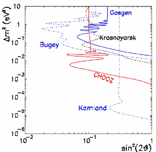
because the neutrino has not enough energy in the laboratory frame to produce the associated charged lepton. Therefore oscillation experiments performed at reactors are disappearance experiments. They have the advantage that smaller value of ∆m2 can be accessed due to the lower neutrino beam energy. Table 1.2 shows the limits on Pee from the null results of Gosgen [45], Krasnoyarsk [46], Bugey [47] and CHOOZ [40], [41]. In particular, CHOOZ is the first LBL (“long baseline”) reactor experiment. With a baseline of 1000 m and a mean energy of 3 MeV, CHOOZ is sensitive to the lowest value of ∆m2, so that it can cross-check information from atmospheric neutrinos and the upper sector of the LMA solutions for solar neutrinos. No evidence was found for a deficit in the neutrino flux; this null result translates to exclusion regions in the (∆m2, sin2 2
θ
) plane shown in Figure 1.10. The 90% CL limits include ∆m2< ×7 10−4eV2 for maximal mixing and sin 22 θ <0.10 for large ∆m2. The CHOOZ results are significant in excluding part of the region that corresponds to the LMA solution of the solar neutrino problem. Furthermore, the CHOOZ bounds rule out with high significance the possibility that νµ→ νe oscillations explain the atmospheric neutrino deficit.Figure 1.10: Excluded regions at 90% for νe oscillations from reactors experiments and the expected sensitivity from the KamLAND experiment.
Neutrino physics overview ___________________________________ -17-
Experiment L Limit ∆m2min (eV2)
Bugey 15.40 m >0.91 10-2
Gosgen 38, 48 , 65 m >0.9 0.02
Krasnoyarsk 57.230 m >0.93 7 × 10⁻³
CHOOZ 1 Km >0.95 7 × 10⁻⁴
KamLAND 150-210 Km >0.85 7 × 10⁻⁵
Table 1.2: 90% CL lower bound on Pee and Δm2 sensitivity from searches at reactor experiments.
1.3.3.b.Neutrinos from accelerators
Conventional neutrino beams from accelerators are mostly produced by π decay, with the pions produced by the scattering of the accelerated protons on a fixed target (graphite, beryllium..); hadron decays produce muons and muonic neutrinos. The final composition and energy spectrum of the neutrino beam is determined by selecting the sign of the decaying π and by stopping the muons produced in the beam line.
SBL experiments
Most oscillation experiments performed so far with neutrino beams from accelerators have characteristic distances of the order of hundreds of meters (short baseline or SBL experiments). Such experiments are not sensitive to the low values of ∆m2 invoked to explain either the solar or atmospheric neutrino but they are relevant for 4-ν mixing schemes.
The CHORUS [53] experiment at CERN searched for νµ ↔ ντ oscillations by looking
for τ decays from charged-current ντ interactions. The emulsion target of the detector,
having a resolution of about a micron, enables the detection of the decay topology of the
τ. After having analyzed a sample of 126000 events containing an identified muon and
7500 purely hadronic events, no ντ candidate has been found. This result translates in a
limit on the mixing angle sin22θµτ < 8 × 10⁻⁴ at 90% C.L. for large ∆mµτ2 .
The only positive signature of oscillations at a laboratory comes from LSND [48] (Liquid Scintillator Neutrino Detector) which presented the evidence for νµ →νe at
∆m2∼1 eV2. This result cannot be accommodated together with solar and atmospheric neutrino oscillations even in the framework of four-neutrino mixing, in which there are three light active neutrinos and one light sterile neutrino. The region of parameter space that is favoured by the LSND observations has been almost completely excluded by other experiments like KARMEN [49], CCFR [50] and NOMAD [51].
The MiniBooNe [52] experiments searches for νµ→νe oscillations and is specially designed to draw a conclusive statement about the LSND neutrino oscillation evidence.
Neutrino physics overview ___________________________________ -18-
The first results were shown and published at the beginning of the summer 2007. As shown in Figure 1.11 the LSND 90% CL allowed region is excluded at the 90% CL. The MiniBooNE’s results, therefore, rule out a fourth sterile neutrino, thereby verifying the current Standard Model with its three low-mass neutrino species. On the other hand a new anomaly showed up: there were more electron neutrino events detected at low neutrino energies than expected; several possible explanations have been envisaged, the energy spectrum distortion not being compatible with a 3-flavour neutrino oscillation. Further analysis is planned using the MiniBooNE antineutrino sample and a new experiment, MicroBooNE, has been approved at Fermilab to explore this low energy anomaly.
In addition, another experiment, SciBooNE, was set up during the 2007-2008 period, when a second fine-grained detector was placed much closer to the Booster neutrino beam source. SciBooNE will not only allow precision cross section measurements but also can be used as a near detector in conjunction with MiniBooNE to explore muon neutrino disappearance oscillations with better sensitivity.
MiniBooNE represents the first phase for the BooNE experiment, which should use a muon-neutrino beam to determine whether muon neutrinos oscillate to electron neutrinos. In addition to neutrino oscillations. BooNE is also sensitive to other phenomena, such as supernova explosions and the decay of exotic particles.
Figure 1.11: The MiniBooNE 90% CL limit and sensitivity (dashed curve) for events with 475 < EvQE < 3000 MeV within a two neutrino oscillation model. Also shown is the limit from the boosted decision tree analysis (thin solid curve) for events with 300 < EvQE <3000 MeV. The shaded areas show the 90% and 99% CL allowed regions from the LSND experiment.
Neutrino physics overview ___________________________________ -19-
LBL experiments
Smaller value of ∆m2 can be accessed using accelerator beams for long baseline experiments (LBL). In such experiments an intense neutrino beam from an accelerator is aimed at detector (usually) located underground at several hundred kilometres far away. The minimum goal of these experiments is to test the presently allowed solution for the atmospheric neutrino problem by searching for either νµ disappearance or ντ appearance.
The first LBL experiment was K2K [54], [55](KEK to Kamiokande): a pure νµ beam with mean energy of about 1.3 GeV was sent from KEK to the SK (SuperKamiokande) detector, located L = 250 km away in the Kamioka mine. Since the beam is pulsed, SK can discriminate atmospheric νµ from KEK νµ. The 2004 K2K results, shown Figure 1.9, are consistent with the expectations based on SK atmospheric data and contain a 4σ indication for oscillations.
The most important K2K result is the energy spectrum: K2K is competitive on the determination of ∆m2atm because, unlike SK, K2K can reconstruct the neutrino energy and data show a hint of the spectral distortion characteristic of oscillations. As a consequence K2K suggests a few different local best-fit values of ∆m2atm , and the
global best fit lies in the region suggested by SK.
The running MINOS [44] experiment, showing several similarities to K2K, is designed to detect neutrinos delivered by the Main Injector accelerator at Fermilab (NuMI) with average energies of about 5-15 GeV depending of the beam configuration. Two detectors, functionally identical, will be placed in the NuMI neutrino beam: one at Fermilab and the second one at the Soudan mine, 732 Km away. The near detector allows predicting the non-oscillated flux; the far detector allows to discriminate particles from anti-particles, and to discriminate NC from CC scatterings.
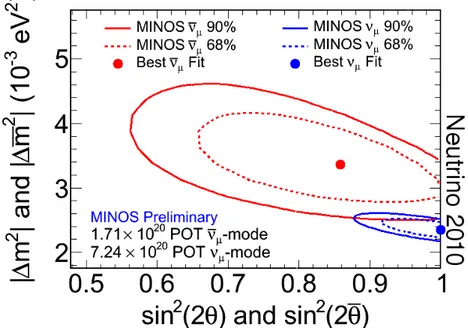
Like K2K data, those from MINOS also contain a hint of the spectral distortion predicted by oscillations (see Figure 1.12) the data disfavour no oscillations by 6.3 standard deviations. The best fit of the data (see Figure 1.13), in the hypothesis of two-flavour oscillations, give:
2 0.45 3 2 0.40 (3.36 ( ) 0.06( )) 10 m + − stat syst − eV ∆ = ± × 1.18 2
sin 2
θ
=0.86 0.11(± stat.) 0.01(± syst) 1.19Another LBL experiment is OPERA [56], which is the subject of this thesis. OPERA is designed to search for νµ→ντoscillations in the Gran Sasso Laboratory. It will study the interactions of neutrinos with an average energy of 17 GeV, produced at CERN. The goal is to observe the appearance of ντin a pure νµbeam.
From the beginning of 2010, the T2K experiment will send a beam of muon-neutrinos from Tokai (on Japan East coast), 300km across the country to a detector at Kamioka. The beam is designed so that it is directed about 2.5 degrees away from the SK detector (it’s “off-axis” ). The primary goal of T2K is a measurement of θ13 through νe appearance analysis, in addition to improving current estimates for ∆m223 and θ23
Neutrino physics overview ___________________________________ -20-
from νµ disappearance. In doing this, T2K is also expected to yield an important
contribution to the current knowledge of neutrino-nucleon scattering cross-sections.
Figure 1.12: This plot compares the events in MINOS Far Detector (black points) to the expected antineutrino energy distribution in the absence of (anti)neutrino disappearance (red histogram). The data disfavour no oscillations at the 6.3 standard deviation level. [57]
Figure 1.13: Confidence Interval contours in the fit of the MINOS Far Detector antineutrino data (red) to the hypothesis of two-flavor oscillations. The solid (dashed) curves give the 90% (68%) contours. The best fit point is Δm2=(3.36+0.45-0.40 (stat.) ±0.06 (syst.) )x10-3 eV2 and sin2(2Θ) =0.86 ±0.11 (stat.) ±0.01 (syst.). Also shown are preliminary contours from the MINOS neutrino analysis [57].
Neutrino physics overview ___________________________________ -21-
1.4.
The global oscillation picture
As discussed in the previous sections, neutrino oscillations give no information about the absolute value of the neutrino mass squared eigenvalues mi2 (being sensitive only to differences). There are two ordering schemes for neutrino masses that are consistent with the explanation of the atmospheric and solar data as result of neutrino oscillations. The normal (inverted) hierarchy is the one for which the neutrinos separated by atmospheric (solar) mass splitting are heavier than those separated by the solar (atmospheric) mass splitting, as shown in Figure 1.14. As explained in section 1.1.2, the neutrino mixing matrix contains 3 mixing angles: two of them (θ23 and θ13) produce oscillations at the larger atmospheric frequency, one of them (θ12) gives rise to oscillations at the smaller solar frequency.
In summary, evidence for neutrino oscillations comes from a wide variety of sources, and the current status of all neutrino oscillation experiments is summarized in Figure 1.15 although this picture is rather crowded, the allowed atmospheric region can be identified by its high value of ∆m2 ≈2.4 10× −3eV2 corresponding to the region labelled “SuperK 90/99 %” in Figure 1.15. The allowed solar region can be identified from its value of ∆m2 ≈ ×8 10−5eV2, corresponding to the intersection of the upper SNO region with the thin upper KamLAND region in Figure 1.15.
The best world estimates on neutrino masses and mixings from oscillation data are summarised in Table 1.3:.
Figure 1.14: Alternative neutrino mass patterns that are consistent with neutrino oscillation explanation of the atmospheric and solar data. The pattern on the left (right ) is called normal (inverted) pattern. The coloured bands represents the probability of finding a particular weak eigenstate ve, vµ, vτin a particular mass eigenstate. The absolute scale of neutrino masses is not fixed by oscillation data and the lightest neutrino mass may vary form 0.0 -0.3 eV.
Neutrino physics overview ___________________________________ -22-
Figure 1.15: The regions of squared-mass splitting and mixing angle favored or excluded by various experiments.
Parameter Best fit 2σσσσ 3σσσσ 4σσσσ
2 5 2 21 10 m − eV ∆ 7.9 7.3-8.5 7.1-8.9 6.8-9.3 2 3 2 31 10 m − eV ∆ 2.6 2.2-3.0 2.0-3.2 1.8-3.5 2 12 sin θ 0.30 0.26-0.36 0.24-0.40 0.22-0.44 2 23 sin θ 0.50 0.38-0.63 0.34-0.68 0.31-0.71 2 13 sin θ 0.000 ≤0.025 ≤0.040 ≤0.058
Table 1.3: Best-fit values, 2σ, 3σ and 4σ intervals for the three-flavour neutrino oscillation parameters from global data including solar, atmospheric, reactor and accelerator experimenst.
Chapter 2
The OPERA Experiment
The OPERA (Oscillation Project with Emulsion- tRacking Apparatus) experiment [56] was designed to perform a conclusive test to check the νµ↔ ντ oscillations hypothesis. It was motivated by results from atmospheric neutrino experiments; hence, its sensitivity covers the ∆m2 region allowed by atmospheric neutrino data. The goal of the experiment is to observe the appearance of ντ in an initially pure beam of νµ. The observation of even a few ντ events will be significant, because of the very low expected background.
In this chapter, the experimental setup and the physical performance of OPERA are briefly described.
2.1.
The conceptual design of OPERA
The CNGS, a pure muonic neutrino beam [58], travels from CERN towards the Gran Sasso Laboratory (730 Km away – Figure 2.1 where the OPERA detector is placed. If oscillation occurs, ντinteractions are likely to happen; kinematical analysis is performed to discriminate background events (νµ CC/NC interactions) from the signal (ντ CC interactions). The search for appearance of ντrequires the detection and identification of the charged lepton by its decay pattern. Because of its short mean-life (2.9 × 10⁻¹³ s - cτ ∼ 87
µ
m), a very high resolution tracking device is needed. Nuclear emulsionsfeature a sub-micron spatial resolution, therefore are suitable for the purpose. This device was used in the CHORUS experiment, which also searched for neutrino oscillations and, later, in DONUT. Unlike CHORUS [53], in which the target was made only of emulsion plates, the OPERA design is based on the Emulsion Cloud Chamber (ECC), a modular structure made of passive plates (lead, in this case) interleaved with
The OPERA Experiment ___________________________________ -24-
emulsion plates. The so-called cell, made of a thin lead plate and emulsion layer, combines the high precision tracking capabilities of nuclear emulsions and the large target mass given by the lead plates. By piling-up 56 cells in a sandwich-like structure one obtains a brick; by assembling a large quantity of such modules, it is possible to realise a detector optimised for the study of ντ appearance.
This target is complemented with arrays of electronic trackers for the real time determination of the event position and with magnetised iron spectrometers for muon identification and for the estimation of their charge and momentum.
Figure 2.1: Schematic view of the neutrino beam trajectory. The beam is produced at CERN. The detector is located in the Gran Sasso Laboratory, about 730 km away.
The OPERA Experiment ___________________________________ -25-
2.1.1.
Experimental setup
2.1.1.a.The CNGS beam
The CNGS (CERN Neutrino to Gran Sasso) beam [58] is designed and optimised for the study of νµ↔ ντoscillations in appearance mode by maximizing the number of charged current ντinteractions at the LNGS site.
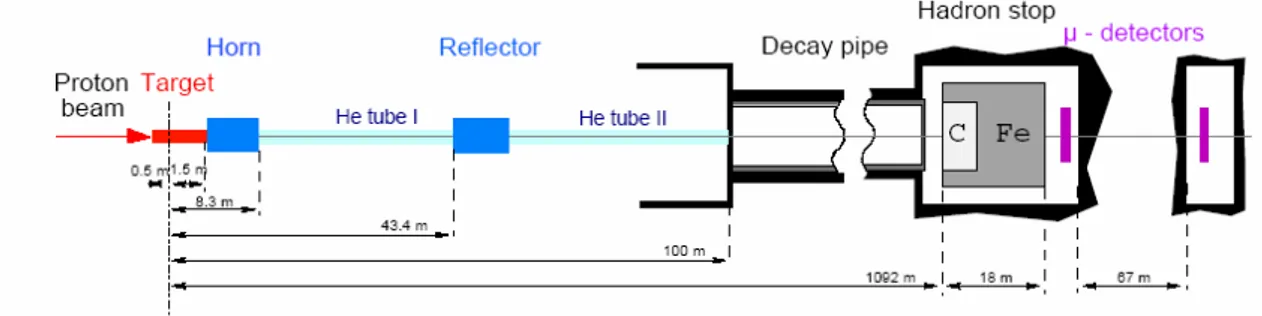
A 400 GeV proton beam is extracted from the CERN SPS and sent into a target made up of several thin graphite rods. Secondary interaction products (pions and positive kaons) are focused into a parallel beam by a system of two magnetic lenses (“horn” and “reflector”).
In a long decay pipe these particles yield muon-neutrinos and muons. The remaining hadrons are absorbed by an iron beam stop. Muons are absorbed further downstream in the rock, while the neutrinos continue to travel to Gran Sasso (Figure 2.2). Due to Earth curvature, the neutrino beam reaches the detector with an angle of about three degrees with respect to the horizontal plane.
Table 2.1 summarizes some beam features. The average neutrino energy at LNGS location is 17 GeV. The νµ contamination is about 2.1 % and the ντ-prompt (coming from Ds decay) contamination is negligible. The
ν ν
e+ e contamination is lower than 1%allowing to probe also the sub-dominant oscillation channel νµ↔ νe, although with a non-optimised sensitivity. In Figure 2.3 the expected flux (at the LNGS site) of muonic neutrinos is reported.
Assuming a CNGS beam intensity of 22.5×10¹⁹ p.o.t (protons on target) per 5 year, about 23600 νµ CC+ NC interaction are expected and about 205
ν ν
e+ e CC interaction. In the hypothesis of maximal mixing and ∆m2 = 2.5 × 10⁻³ eV2 , about 115 ντ CC interactions should be produced. Considering the τ detection efficiency (Section 2.2.2) about 10 of them should be detected.ν
µ (m-2/pot) 7.45 × 10⁻⁹ν
µCC events/pot/kton 5.44 × 10⁻¹⁷ E µ ν (GeV) 17 / e µν ν
0.8% / µ µν ν
2.0% / e µν ν
0.05%The OPERA Experiment ___________________________________ -26-
Figure 2.3: CNGS v - energy spectrum and oscillation probability multiplied by the vτ cross section
2.1.1.b.The detector
The OPERA apparatus is a hybrid structure made of electronic devices and nuclear emulsions [59]. The former are needed to select the brick where the interaction took place, to identify the muon tracks and to determine their charge and momentum; nuclear emulsions are used as high-precision tracking planes in the neutrino interaction vertex region.
The OPERA detector has two identical substructures, named supermodules (SMs). Each supermodule consists of about 77350 ECC bricks assembled in planar structures called
walls, orthogonal to the beam direction. Each wall is followed by the two planes of
scintillating fibers of the Target Tracker (TT) [60]; a module in OPERA terminology is the complex of a brick wall + its two TT planes. A supermodule is made of 29 modules followed by a muon spectrometer (Figure 2.4) [59].
The target
As mentioned above, the OPERA target part is modular; each wall contains about 2668 bricks for a total of 154750 bricks in the whole apparatus. The brick support structure is designed to insert or extracte bricks from the sides of the walls by using an automated manipulator (BMS).
Each brick has transverse dimensions of 10.2 ×12.7 cm2, a total thickness of about 7.5 cm (corresponding to ∼ 10 X0) and a weight of 8.3 Kg [56]. Its structure is obtained by
The OPERA Experiment ___________________________________ -27-
stacking 56 lead plates (1-mm thick) interleaved with thin emulsion films. Each film has about 44 µm thick emulsion layers on both sides of a 205 µm thick plastic base2.
The dimensions of the bricks are set by different requirements:
• each brick should account for a small fraction of the total target mass: when one or more bricks are selected and removed the total mass must not decrease too much;
• transverse dimension should to be larger than uncertainties in the interaction vertex position predicted by electronic trackers;
• the brick thickness must be large enough to allow electron identification thorough EM showers and momentum measurement of hadrons by multiple Coulomb scattering. Electron identification requires about 3 - 4 X0 and the multiple scattering requires 5÷10 X0; with 10 X0, for half of the events such measurements can be done within the same brick where the interaction took place, without the need to follow tracks into downstream bricks.
The Target Tracker strips help restrict the region of the film to be scanned to locate the interaction; they are arranged in two planes oriented along the X and Y directions, close to the wall.
In order to reduce the emulsion scanning load, Changeable Sheets (shortened as CS in the following) were introduced in OPERA [61]. CS doublets are attached to the downstream face of each brick and can be removed without opening the brick. Charged particles from a neutrino interaction in the brick cross the CS doublet and produce a trigger in the TT scintillators. After a trigger, the brick is extracted and its CS doublet is developed and analysed in the scanning facilities at LNGS or in Japan; the information from the CS is used for a precise prediction of the position of the tracks in the most downstream films of the brick, easing track identification and scanback to locate the neutrino vertex point.
Figure 2.4: Left: schematic drawing of the OPERA detector; Center: sketch of 2 modules; each of them is made of a wall + two Target Tracker planes; Right: real brick picture. CSs sheet are contained in a separate box (white in the image)
The OPERA Experiment ___________________________________ -28-
The muon spectrometer
Muon identification, charge assignment and momentum measurement are performed by the muon spectrometers [62]. Each spectrometer consist of a dipolar magnet made of two vertical walls with rectangular cross sections where the magnetic field is approximately uniform. Each wall consist of iron layers interleaved with planes of Resistive Plates Chambers (RPCs) [63], providing tracking inside the magnet, and range measurement of stopping particles.
Drift- tubes (Precision Trackers) are located in front and behind the magnet as well as between the two walls, to measure the muon momentum and for the precise measurement of the muon-track bending.
In order to solve ambiguities in the spatial reconstruction of tracks, each of the drift-tube planes of the PT upstream of the dipole magnet is complemented by an RPC plane with two 42.6° crossed strip-layers called XPCs. RPCs and XPCs also yield a precise start signal to the PTs.
2.1.2.
Operation mode
With the CNGS beam on, the data rate from events due to neutrino interactions is in correlation with the beam spill. Because of the long distance from the source, synchronization with the spill is done off-line via GPS. The detector remains sensitive during the inter-spill time and runs in triggerless mode. Events detected out of the beam spill are used for monitoring.
The decision on which bricks need removal after a neutrino interaction is based on information from electronic detectors (see Figure 2.5) [65]. The most likely brick is extracted by BMS and the CS doublet is removed, exposed to X-ray to produce references, then developed to be sent to either CS scanning station (at LNGS and in Japan). The brick is stored underground waiting for CS feedback. If the CS doublet does not show tracks of particles produced in the interaction, another CS is attached to brick, it returns to the detector and the second most likely brick is extracted.
In case of positive result of the CS doublet scanning, the brick is brought to a location at a shallow depth outside the underground hall and exposed to the cosmic muon flux High-energy penetrating tracks provide a pattern for accurate alignment (sub-micron precision) of the emulsion films within a brick. The component of electromagnetic showers in cosmic rays and soft muons are suppressed by a 40 cm iron shield above the bricks [64].
In addition to the X-ray marking performed while the CS box is still in contact with the brick, another set of X-ray marks is added to bricks to be developed before they are disassembled: this set provides a first coarse alignment (about 20 µm precision) without the need to scan any track. The brick is unpacked, each emulsion sheet is labelled with an ID number and developed in an automatic plant. Emulsion films are then sent from the Gran Sasso Laboratory to the scanning laboratories that take care of vertex location and study. Each of them uses one of the two automatic scanning systems, respectively named ESS (European Scanning System) [66] and S-UTS (in Japan) [67], that were developed for OPERA.
The OPERA Experiment ___________________________________ -29-
Even when the right brick has been extracted for an interaction, the removal of additional bricks, downstream of the one with the primary interaction, may be required for a complete kinematical analysis of decay candidate events.
The OPERA Experiment ___________________________________ -30-
2.2.
Physics Performance
2.2.1.
Signal and background
The signal of the occurrence of νµ→ντ oscillations is the CC interaction ντN→τ-X. The τ in the final state is detected through the decay topology and its decay modes to electron, muon or single-prong hadron [56]:
( . . 17.8%) e e τ B R τ−→ −ν ν = 2.1 ( . . 17.7%)B R τ µ
τ
− →µ ν ν
− = 2.2 0 ( ) ( . . 49.5%) h τn B R τ− → −ν π = 2.3The multi-prong hadronic decay channel has been disregarded because of a higher background from hadronic interactions The single-prong decay is characterized by a
kink topology.
The criterion used to select a kink candidate is independent of the τ decay channel, but it
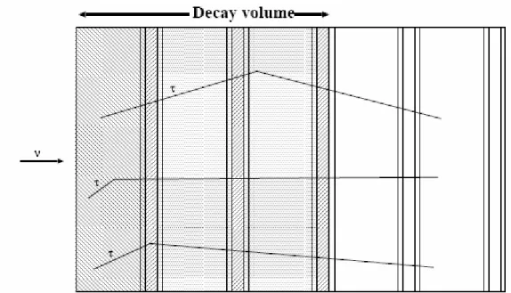
depends on where decays occur. τ decays can be classified as short or long depending
on the decay vertex position with respect to primary vertex (Figure 2.6).
Short decays take place in the same lead plate where the primary vertex is found (about
60%). In this case, there is no chance to reconstruct the parent track and an impact parameter method is applied. The track that is candidate to be a τ-decay daughter is selected and if its impact parameter with respect to the measured primary vertex is larger than a given value (10 micron) a short kink topology has been found and a more
accurate analysis has to be performed.
Long decays are events in which the τ track is long enough to exit the lead plate where
the primary vertex occurs. In this case, at least one film is measured also for the parent track. The topology is considered “interesting” if parent and daughter track cross (within measurement errors), giving significant kink angle. The angular resolution of 2.1 mrad in one emulsion film implies a minimum detectable kink angle of 3.0 mrad.
Events with θkink ≥ 3 × 3.0 mrad = 9.0 mrad [56] are selected, and they undergo further
analysis (which may also include further scanning).
Several techniques are used to define the nature of daughter track. In the electronic channel, the daughter is identified through the electron showering in the ECC. The main background source are charm decays in electronic channel with an undetected primary muon (see Figure 2.7 A)
For the muonic decay mode, the presence of a penetrating (and often isolated) track allows easy identification of the muon attached to the decay vertex. In this case, the background comes from large angle scattering of muons produced in νµCC interactions
The OPERA Experiment ___________________________________ -31-
and from muonic decay of charm particles in the case in which the muon at the primary vertex goes undetected and muon charge assignment is wrong (Figure 2.7 B).
Hadronic decay modes have the largest branching ratio, but they are affected by high background sources:
• One-prong decays from charm particle (with muon at primary vertex undetected) - see Figure 2.7 C.
• Hadron reinteractions (see Figure 2.7 D). In a νµCC event in which muon is undetected or in a νµNC event, a hadron from primary vertex may interact in the lead plate closest to primary vertex. If the other products of this interaction are not detected, the topology found is similar to the CC – single prong decay of the
τ.
Table 2.2 reports the expected background for different decay modes normalized to 106 DIS events.
Figure 2.6: Different decay topologies; short decay (left-hatched region); long decays in base (right-hatched region); long decays outside the base (shaded region); very long decays (white region), not shown.
![Figure 5.3: Multiplicity of photons produced in the interaction of a beam of 5 GeV pions with 1 mm of lead before (left) and after (center) the kinematical cuts and their energy after the cuts (right) [83]](https://thumb-eu.123doks.com/thumbv2/123dokorg/7206211.76099/89.892.161.794.670.878/figure-multiplicity-photons-produced-interaction-center-kinematical-energy.webp)
![Figure 5.8: An example of a hadron interaction reconstructed in a brick exposed to 4 GeV/c hadronic beam.[88]](https://thumb-eu.123doks.com/thumbv2/123dokorg/7206211.76099/95.892.180.757.597.1027/figure-example-hadron-interaction-reconstructed-brick-exposed-hadronic.webp)