Department), Viale Porto Torres, 119; I-07100 Sassari, Italy Received: 27-XII-2013 – Accepted: 4-XII-2014 –Original version Correspondence to: [email protected]
Abstract
In the last two decades of the 20thcentury, most meteorological networks replaced traditional
mechanical thermometers (usually placed inside a Stevenson screen) with electronic ones (usu-ally in the open air, protected by a plastic shelter). Impacts of such instrumental change on the climatology of daily minimum and daily maximum temperatures are assessed here, by analysing eleven years of data from a couple of stations operating in parallel in the same test site in a lo-cation with a Mediterranean climate. Seasonal effects (i.e. monthly biases ranging from -0.8 C to +1 C) were detected on maximum temperatures, but they compensate each other in the yearly average. In minimum temperatures, electronic thermometers introduced a -0.75 C bias, regard-less of the season. Specific biases due to horizontal winds and to vertical heat fluxes were also detected and studied. Two possible causes of the climatological bias were investigated: local wind conditions and different responses to turbulent heat fluctuations by electronic and mechan-ical thermometers. Other possible causes exist, but they could not be investigated due to a lack of data. The present study shows that, in the test site, replacing traditional thermometers with modern ones in climatological networks introduced an underestimate in minimum temperatures. This suggests that in locations with similar microclimates the real atmospheric warming could be even greater than that observed to date.
Key words: Mechanic thermometers, electronic thermometers, climatology, time series, Mediterranean
1 Introduction
For about three centuries, meteorological services or other institutions dedicated to regularly observing tempera-tures measured this fundamental quantity by means of ana-logical instruments. A clear description of how mechan-ical thermometers work can be found in publications by the World Meteorological Organization (Simidichiev, 1986; WMO, 2008) or in many other textbooks.
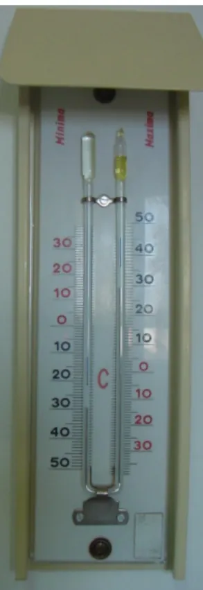
The most familiar thermometer is the mercury ther-mometer, originally invented by Fahrenheit in 1721 and im-proved over the following centuries. Figure 1 shows a mod-ern version of a minimum-maximum mercury thermometer.
In the 20thcentury, mechanical thermographs became
very popular, as well. These instruments had a bi-metallic sensor inside that would plot a pen writing on a paper graph,
like the one in Figure 2. The thermograph contained a slowly rotating cylinder (covering a seven-day period) to be able to continuously record temperatures on a weekly basis.
Thermographs and mercury thermometers were not usu-ally installed in the open air, but were placed inside wooden screens, the so-called Stevenson Screen, of various kinds.
Both types of instruments were used by meteorological services for a long time to register the series of minimum and maximum temperatures that are the basic records for long-term climate studies. The quality of these time series has always been a major concern for climatologists.
One problem, addressed by Parker (1994), was the his-torical setting of these instruments. In his work, he compared the effect of the different screens used to house thermometers during the 19thand 20th centuries. A result that is useful
Figure 1. Traditional liquid-in-glass (mercury) min-max
ther-mometer.
screen, i.e. 0.2 C to 0.5 C, depending on the experiment and the period of the year.
The problem of discontinuity due to relocation or to poor maintenance was then addressed in a set of interesting studies by an Italian research group (Brunetti et al., 2000 and 2006; Maugeri and Nanni, 1998) which assessed the quality of temperature time series and applied a homogenisation pro-cedure to create sets of homogenous secular time series for climate studies. A similar piece of research was carried out by Peterson and Easterling (1994) and by others not quoted here.
In the last decades of the 20thcentury, electronic
ther-mometers were introduced, usually based on thermistors or on thermocouples. By the end of the century, most mechani-cal thermometers had been abandoned. Details on how elec-tronic instruments work and general rules for data process-ing can also be found in World Meteorological Organization publications (Simidichiev, 1986; WMO, 2008).
Analyses on the performance of some types of elec-tronic thermometers can be found in literature. Cheney and Businger (1990), for example, studied thermocouple ther-mometers, showing that they are very sensitive to fast tem-perature variations.
More recently, Lin and Hubbard (2004) analysed intrin-sic errors in four networks using two types of sensors: ther-mistors and platinum resistance thermometers. When the whole set of measurements (-25 C to +50 C) was
consid-ered, an error varying from 0.2 C to 0.33 C was detected in temperature estimates. At temperatures lower than -20 C or greater than +30 C, greater errors were found, possibly by as much as 1 C.
At the beginning of the 1990s, Quayle et al. (1991) and Wendland and Armstrong (1993) analysed the possi-ble propossi-blems of the major instrumental change described above, by comparing liquid-in-glass analogical thermome-ters with electronic resistance-based (thermistors) ther-mometers. Quayle et al. (1991) highlighted a slight bias in minimum temperatures of about +0.3 C; both studies no-ticed a slight bias in maximum temperature (either -0.4 C or -0.6 C). Overall, then, electronic thermometers based on thermistors register narrower daily ranges (0.6 to 0.7 C) than the ones usually observed by traditional liquid-in-glass ther-mometers.
The different performance of electronic thermometers is the consequence of the response time of their sensors that is known to be of the order of a few seconds as compared to the one of mechanical sensors that take minutes to respond to temperature variations (Stringer, 1972). The potential risk of such an instrumental change was pointed out by the World Meteorological Organization in WMO (2008).
The issue of the impact of this instrumental change on climatology, however, must also be addressed from another point of view. Modern electronic thermometers are generally operated by data loggers, which only record a finite set of measurements, generally compliant with World Meteorolog-ical Organization recommendations (WMO, 2008).
Apart from weather stations designed to measure turbu-lence, data loggers usually take a measurement (or a set of measurements) every few minutes or even every hour. Min-imum and maxMin-imum temperatures, thus, turn out to be the minimum and the maximum of such a finite set of values, rather than the lower and the upper band of a continuous measurement, as used to be the case with mechanical ther-mometers.
It is very likely that such a different way of estimating extreme daily temperatures, combined with the highest ac-curacy of thermocouples, is far from being irrelevant from a climatological point of view. The higher accuracy of thermo-couples, for example, is likely to produce different effects in different boundary layer conditions. In fact, rapid changes in air temperature are likely to be observed by a thermocouple, while a bi-metallic or a mercury-in-glass thermometer would not respond as accurately.
This piece of research intends to investigate this prob-lem, by comparing about ten years of maximum and min-imum temperatures in one location of Sardinia (Italy) that has been housing three weather stations installed in the same field: a historical mechanical station installed in 1959, still in operation, and two electronic stations installed in the mid-1990s. The climate of Sardinia and the specific climate of the test location are typically Mediterranean, i.e. a Csa climate according to the K¨oppen-Geiger classification (Peel et al., 2007).
Figure 2. Paper strip from a mechanical thermograph.
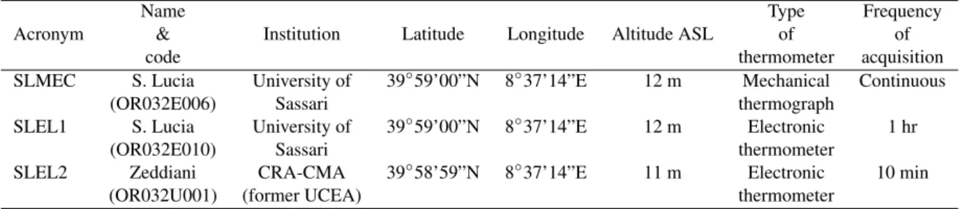
Table 1. Information recorded by the weather stations. Names and codes follow internal ARPAS regulations; the acronyms SLMEC, SLEL1
and SLEL2 are used throughout the paper.
Name Type Frequency
Acronym & Institution Latitude Longitude Altitude ASL of of
code thermometer acquisition
SLMEC S. Lucia University of 39 59’00”N 8 37’14”E 12 m Mechanical Continuous
(OR032E006) Sassari thermograph
SLEL1 S. Lucia University of 39 59’00”N 8 37’14”E 12 m Electronic 1 hr
(OR032E010) Sassari thermometer
SLEL2 Zeddiani CRA-CMA 39 58’59”N 8 37’14”E 11 m Electronic 10 min
(OR032U001) (former UCEA) thermometer
In the first part, this study estimates the statistical pa-rameters of temperature differences between nearby stations: average, standard deviation and RMS (root mean square er-ror). The analysis is conducted on both a yearly and a monthly basis. In the second part of the study, the author in-vestigates whether the surface wind or the vertical heat flux from the surface layer play a role.
2 Description of stations and datasets
In 1959, the Department of Agronomy of the University of Sassari installed a weather station in one of its own exper-imental fields in Sardinia: S. Lucia (near Oristano). The sta-tion consisted of a Stevenson screen, housing a thermograph based on a bi-metallic thermometer, a mercury thermometer and a pluviometer. The station has been operating continu-ously since then.
The site is well exposed and far away from urban ar-eas; the field has been cared for continuously and the station has received very good maintenance. As far as the author is aware, it is one of the best weather stations existing in Sar-dinia.
In 1996, the University installed an electronic station next to it. An air thermometer (based on a thermocouple), a terrain surface thermometer, an anemometer, a pyranometer and a few more instruments were installed; the air
thermome-ter is 2 m above ground level, it is inside a standard parallel cone shield and it is ventilated.
All the station measurements were recorded on an hourly basis. Though maintenance was good, there have been some interruptions over the years.
In the 1990s, the former Italian Central Office of Agrar-ian Ecology (UCEA) installed one more station with sev-eral instruments (including a 2 m thermometer based on a thermocouple) in the same field as S. Lucia, only a few dozen metres from the two stations of the University of Sas-sari. Its own data logger measures the temperature every ten minutes; the daily maximum and the daily minimum temperature are thus calculated among 144 instantaneous values.
The setting of this new electronic thermometer was sim-ilar to the previous one: it was installed 2 m above the ground, it has a standard parallel cone shield and it is ven-tilated.
This new station was also provided with a surface ther-mometer, i.e. an electronic thermometer installed right over the ground, protected by a small metallic shelter. This mea-surement is fundamental to know the temperature at the in-terface between the ground and the air.
The station sites and the instrumental history of the S. Lucia field make it very interesting for climatological analy-ses that aim to highlight instrumental effects.
Figure 3. Scatter plot of the SLMEC-SLEL2 minimum (a, left) and maximum (b, right) temperatures over time. Gaps in the plot correspond
to rejected or missing data.
Table 2. Statistics of differences in minimum temperatures (Tmin) and maximum temperatures (Tmax) at S. Lucia stations. Acronyms
SLMEC, SLEL1 and SLEL2 are explained in Table 1. The errors of the means are the 3-sigma of the estimator probability distributions, i.e. they indicate the range of the 99.7% confidence level.
Mean Standard Deviation RMS Sample size Tmin (SLMEC) Tmin (SLEL1) +0.41 ± 0.05 C 0.97 C 1.05 C 3017 Tmin (SLEL1) Tmin (SLEL2) +0.46 ± 0.05 C 0.85 C 0.97 C 2305 Tmin (SLMEC) Tmin (SLEL2) +0.75 ± 0.06 C 1.02 C 1.61 C 3102 Tmax (SLMEC) Tmax (SLEL1) +1.10 ± 0.06 C 1.09 C 1.54 C 3017 Tmax (SLEL1) Tmax (SLEL2) -1.06 ± 0.07 C 1.07 C 1.50 C 2305 Tmax (SLMEC) Tmax (SLEL2) -0.06 ± 0.06 C 1.11 C 1.24 C 3102
The information recorded at all the stations is given in Table 1.
3 Comparisons of full sets
In this analysis, the 1996-2007 temperature time series of the three stations in the S. Lucia site were compared.
Before starting with the analysis, a visual inspection of the three time series was performed, in order to pick up any macroscopic problems in the data. Figure 3 shows differ-ences in minimum and maximum temperature between me-chanical thermograph (henceforth SLMEC) and UCEA elec-tronic thermometer (henceforth SLEL2) measurements dur-ing the whole decade, havdur-ing discarded suspect data.
As one can see, no unrealistic long-term effects appear in the data; even the yearly cycle in maximum temperatures (described in section 4) is stationary throughout the whole period. A few sparse outliers in temperature differences re-main, mostly in 2001 and 2002; however, they affect a very small amount of records and do not have an impact on the present study.
Similar graphics were made to compare the University of Sassari electronic thermometers (henceforth SLEL1) and the other two time series. These extra graphics are not worth
showing here, since they simply confirm the good quality of all the time series.
Table 2 shows the mean, the standard deviation, the RMS and the sample size of all possible different combina-tions between the three time series.
The biases between the time series (estimated using arithmetical means) are quite different, but they can be con-sidered to be precise because of the great size of the sample (2,000 to 3,000 records). It is a known fact that the variance of the estimator of the arithmetical mean is:
2 m= 1 N 2 s (1) where 2
mis the variance of the estimator, 2sis the variance
of the sample and N is its size.
In this specific case, the 1-sigma random error in the bias estimate ranges from 0.01 C to 0.02 C, even lower than the instrumental precision: about 0.1 C in theory and 0.2 -0.3 C according to Lin and Hubbard (2004).
In Table 2, the means are accompanied by the 3-sigma of the probability distribution of the estimator, so they in-dicate 99.7% confidence level. Therefore, from a statistical point of view, the first results here are indeed quite robust.
For both minimum and maximum temperatures, the mean differences between the three S. Lucia time series are
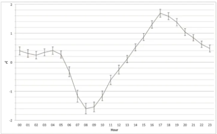
Figure 4. Hourly means of temperature differences between the
two S. Lucia electronic thermometers (SLEL1-SLEL2). The error bars indicate 3-sigma in the estimate of the mean, i.e. the range of the 99.7% confidence level.
very different one from the other. In particular, it can be no-ticed that the temperature range of SLEL1 is much lower than SLEL2 and SLMEC.
This happens because the minima and maxima of SLEL1 are picked from among the 24 instantaneous hourly values, whereas those of SLEL2 are picked from among a denser set of instantaneous records and those of SLMEC are minima and maxima of a continuous analogical signal.
It is clear that the 24-hour sampling technique of SLEL1 is not adequate for registering minimum and maximum tem-peratures. Therefore, from now on, the SLEL1 records will only be used when the 24 instantaneous temperatures are needed; no further considerations will be made regarding the minimum and maximum temperatures of the SLEL1 time se-ries.
Considering that the SLEL2 station is a few dozen me-tres away from the two University of Sassari (SLMEC and SLEL1) ones in the very same field, it was also decided to test if such a small difference in the station setting had any effect on the comparison between the SLEL2 and SLMEC.
In order to test this, mean differences in the SLEL1 and SLEL2 instantaneous temperatures are plotted in Figure 4. The error bars indicate the 3-sigma of the probability esti-mator of the mean, i.e. they indicate the range of the 99.7% confidence level.
The graph shows that the two compare very well on average, except for some positive and negative biases that can be seen morning (07.00 to 10.00 UTC) and mid-afternoon (15.00 to 21.00 UTC). However, such biases drop to 0 C at the time of the day when minimum and maximum temperatures usually occur, i.e. before sunrise and at about 14.00 local time (13.00 UTC).
In fact, when analysing the time of the day when Tmin is record in SLEL2, it happens that 72% of them occur between 00.00 and 07.00, i.e. at the time of day when the average difference between the two time series is within ± 0.4 C. Similar considerations apply to maximum
Figure 5. Monthly means of mean temperature differences (SLMEC-SLEL2): DTmin indicates the difference in minimum temperatures; DTmax indicates differences in maximum tempera-tures. The error bars indicate 3-sigma in the estimate of the mean, i.e. the range of the 99.7% confidence level.
temperatures, as 72% of Tmax occur between 11.00 and 14.00.
The author therefore believes that, if the measurements of both the SLEL1 and the SLEL2 had been continuous rather than discrete, the mean temperature maxima and the mean temperature minima of the two series would have al-most perfectly coincided.
The above result is very important because it allows the author to compare maxima and minima of the SLMEC against those of the SLEL2 as if the two thermometers were placed in the same location. Moreover, the SLEL2 data log-ger takes measurements with the typical frequency of many modern weather stations.
The comparison of the SLEL2 and the SLMEC, is the only one free of the sampling effect. Therefore, for the scope of this piece of research, all the results of the following chap-ters will be based on it.
4 Overall bias and yearly cycle
Table 2 shows that the maximum temperatures of the SLEL2 and the SLMEC coincide quite well on av-erage, with just -0.06 C ± 0.06 C bias (99.7% confi-dence level). On the other hand, minima recorded by me-chanical thermometers are significantly higher than those by electronic ones: +0.75 C ± 0.06 C (99.7% confi-dence level). The temperature range observed with the SLEL2 is 0.81 C greater than the one observed with the SLMEC.
Figure 5 shows the monthly means of the SLMEC-SLEL2. The error bars indicate the 3-sigma of the proba-bility estimator of the mean, i.e. they indicate the range of the 99.7% confidence level. A seasonal cycle is clearly vis-ible in the temperature maxima while no important seasonal effect can be detected in the minima.
Figure 6. Mean temperature differences versus vertical heat gradient. (a, left) Bias of minimum temperature. (b, right) Bias of maximum
temperature.
As one can see, the SLMEC Tmax are higher than the SLEL2 Tmax for the winter months, with a greatest positive bias in December: about +1 C. On the contrary, during the summer months a negative bias is observed, with the lowest value in June: about -0.8 C. As one would expect, the sea-sonal biases of Tmax compensate each other.
Although the results of Table 2 would be enough to show that the change in the thermometer described in section 1 is likely to have introduced a negative climatological bias in the minimum temperature and the seasonal climatologi-cal biases (compensating each other) in the maximum tem-peratures, it is important to investigate the causes of such biases.
Apart from the screening that explains a fraction of it, the main source of the bias is the different response of differ-ent thermometers to local conditions of the planetary bound-ary layer (the so-called PBL). Considering the available data, two forcings can easily be investigated:
• the vertical thermal gradient in the surface layer; • the local wind measured 10 m above the ground.
Other possible forcings, like large-scale advection or ra-diation at different wavelengths, are reasonable to think of, but in the present case, they are difficult to estimate because of lack of data.
If sufficient data and better mathematical models to de-scribe all these effects were available, it is likely they would be able to explain most of the climatological bias and most of the noise in the results.
5 Effect of vertical thermal gradient
It is well known (Stull, 1988) that in the unperturbed PBL, the daily temperature cycle at 2 m above the ground, i.e. the height where thermometers are commonly installed, is mainly driven by the heat released by the ground itself. The latter acts as a black body that releases the heat it has
captured at infrared wavelengths by absorbing the sunlight at visible wavelengths.
The mechanism responsible for the vertical heat trans-port is different from day to night time. During the day, heat plumes rapidly move upward from the ground, feeding the big convective cells called thermals that mix the PBL. At night, the air above ground is vertically stable and the ground nocturnal cooling maintains a downward turbulent heat flux that slowly cools the air layers above.
It could then be interesting to analyse the different ef-fects of the vertical turbulent heat flux on mechanical and electronic thermometers.
While daily PBL turbulence is harder to parameterize, the nocturnal vertical turbulent heat flux (w0z0) is commonly
estimated by a first order closure as in Equation 2: w0z0= k@T
@z (2)
where k is a constant, usually set around 0.5.
More precise estimates of first order turbulence or higher order turbulent closures would require measurements taken with sonic anemometers and ground flux instruments.
Precise values of the vertical temperature gradient in the air layer above ground cannot be obtained with the available data. However, the typical mathematical first order approx-imation, the so-called finite difference, can easily be calcu-lated.
The vertical heat gradient is then estimated by the dif-ference between the air temperature measured at 2 m height (i.e. SLEL2) and the temperature of the microlayer above the ground (the so-called ground surface temperature) divided by the height, i.e.:
@T @z = T2m Ts h + O ⇣ (T2m Ts)2 ⌘ (3) where @T/@z is the vertical gradient, T2m is 2 m
tempera-ture (SLEL2), Tsis the surface temperature measured by the
UCEA station, h is the height of the thermometer (i.e. 2 me-ters) and O⇣(T2m Ts)2
⌘
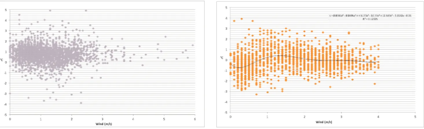
Figure 7. Mean temperature differences versus local wind. (a, left) Bias of minimum temperature versus mean wind speed during the hours
when the air cools down. (b, right) Bias of maximum temperature versus mean wind speed during the time when the air heats up and power law regression with exponent 6 (wind speeds greater than 4 m s 1were discarded).
going to 0 as (T2m Ts)2. Neglecting this error leaves some
noise in the estimate, but it is generally small.
The combined effect of the two approximations de-scribed above makes the estimates of the heat flux rather rough; however are they are the only possible ones.
Figure 6 shows the biases of the SLMEC-SLEL2 Tmin and Tmax versus the vertical temperature gradient estimated with Equation 3. According to Equation 2, Figure 6a could also be considered a scatter plot of Tmin bias versus heat flux scaled by a constant value k.
When examining Tmin (Figure 6a), it appears that @T /@z is more frequently positive than negative, indicat-ing that at night the ground is more often cooler than the air above, though the opposite situation is not infrequent.
Figure 6a also shows a negative linear dependence of Tmin bias on @T/@z. That means that when the air is colder than the ground, the air temperature measured by an electronic thermometer (SLEL2) drops to much lower val-ues than those measured by thermographs (SLMEC). On the other hand, when the ground is much cooler than the air above, Tmin bias tends to 0 C, i.e. both thermometers (SLMEC and SLEL2) respond in the same way.
Figure 6b shows the scatter plot of maximum tempera-tures vs @T/@z. Although Equation 2 does not apply to daily turbulence, the graph is still interesting to analyse.
As one can see, in this figure @T/@z is mainly negative, i.e. in the central hours of the day the ground is generally hotter that the air above. Days when the gradient is positive exist too, but they are much rarer events.
When @T/@z is between -5 C and 0 C, the bias of max-imum temperatures (SLMEC-SLEL2) is low with no evident ties between the two quantities, i.e. when the air temperature and the ground temperature are coupled, the thermographs and the electronic thermometers register similar values.
On the other hand, if @T/@z is lower than -5 C, a weak, noisy negative trend appears. This means that when the ground is much hotter than the air above, the electronic
ther-mometer captures higher temperatures than the mechanical ones.
Finally, fewer considerations can be made during day-time when the ground happens to be not as warm as the air above. On those rare events, it seems that the bias is higher than 0 C, but that is just a rough indication due to the scarcity of data and to their noise.
Overall, it seems that the vertical heat gradient does play an important role in forcing different responses of mechani-cal and electronic thermometers, because of the effects it has on local turbulence.
6 Effects of local wind
The PBL scenario described in section 5 can also be perturbed by surface wind. If the wind blows across a large-scale surface temperature gradient, it transports heat that causes air temperature variations (with an hourly timescale), decoupling it from the ground. This effect is mathematically accounted for by the so-called advection term of the horizon-tal wind equation, i.e. the right hand side term of Equation 4: dT
dt = @T
@t + !v · !rT (4)
Unfortunately, this data is not enough to analyse large-scale advections.
At a local scale, the wind drives small-scale turbulence, especially in the layer closest to the ground. In such a case, the turbulent mixing of the air causes fast temperature fluc-tuations mainly at a timescale of seconds.
Figure 7 shows the effects of 10 m wind on SLMEC-SLEL2 temperature differences. The mean wind intensities are estimated in different ways, according to the time of day when the SLEL2 minima and maxima have been recorded.
According to WMO recommendations, the daily mini-mum temperature is the minimini-mum value between 00.00 and 24.00 Greenwich Mean Time. In Sardinian climate, this
min-imum value mainly occurs a little before sunrise, i.e. be-tween 00.00 and up to 07.00 UTC, although there are many days when it occurs after sunset, i.e. between 16.00 and 24.00 UTC.
On a generic day, then, the minimum temperature is mainly the minimum of the temperatures recorded during the second part of the night before the sunrise of that day (00.00 to 07.00), but it is not infrequent that it should be the min-imum of the temperatures of the first part of the night after sunset (16.00 to 24.00).
In this piece of work, whenever minimum temperatures were registered before sunrise, wind values of Figure 7 were the scalar averages of the wind intensities for the whole night before. Whenever the minima were registered after sun-set, the associated mean winds of Figure 7 were the scalar averages of the afternoon values. This choice is to select the wind blowing when the most effective air cooling takes place.
As far as maximum temperatures are concerned, since they generally occur in the afternoon (usually at 14.00 local time), the associated mean winds of Figure 7 were always calculated by averaging the morning values. As before, this is made to select the wind when the most effective air cool-ing thakes place.
Though Figure 7a is noisy, it seems that the bias in Tmin differences have a mild negative linear dependence on wind speed. It means that during calm nights the bias of the SLMEC-SLEL2 tends to be greater than on windy nights.
The effect on Tmax bias (Figure 7b) turns out to be more complex to describe. In situations when the mean wind speed is lower than 0.5 m s 1the bias of the SLMEC-SLEL2
is slightly negative, going down to about -0.6 C. When the mean speed grows, the bias of Tmax suddenly increases, growing up to almost +0.5 C at speeds of more than 1 m s 1.
At even greater intensities the pattern inverts its trends again and the bias tends towards 0 C, especially beyond 3 m s 1.
This effect is mathematically depicted by applying a high power law polynomial regression to the function join-ing wind speed and Tmax bias, as was shown in Figure 7b. Though the regression is only a statistical description of the phenomenon (there is no physical meaning for such a power law), the curve seems to be able to describe the particular pattern described above.
In conclusion, the effect of local wind is small for Tmin, but it seems to carry interesting insights as far as Tmax are concerned.
In calm wind situations, the mechanical thermometers lose the ability to make precise measurements, as they are affected by the slow thermal mechanical inertial of the in-strument itself. This seems to justify the small Tmax bias, since the slow thermal mechanical inertia of the bimetallic or mercury sensor is actually the feature that takes the measure-ments.
In weak wind situations, the electronic thermometers take precise measurements, but turbulence dominates and that introduces the highest bias.
In strong wind situations, the atmosphere tends toward neutral regimes where turbulence plays a lesser role. This seems to lead all thermometers toward similar value, again reducing the bias in Tmax.
7 Discussion
Biases in minimum/maximum temperature time series at decadal scale can be introduced in four ways: 1) the change of siting of the station; 2) the change of instrument; 3) the screening of the instrument; 4) the sampling frequency and the type of post-processing of the basic information (the instantaneous temperature).
The net effect of the four forcings can sometimes intro-duce severe discontinuities in the time series and climatol-ogists should deal with that before using data for long-term analyses.
In many situations, forcing no. 1) is the main source of bias, but in this experiment it has a minor effect, as dis-cussed in chapter 3. This important initial condition enables this analysis to investigate the effects of forcings 2), 3) and 4). The consequences of forcing no. 4) can have a big im-pact, too, as discussed below.
In this analysis, electronic thermometers operated with data loggers recording one measurement every hour (SLEL1) are not suitable to correctly estimate daily minimum and daily maximum temperatures. In order to do that, the data loggers of the weather station must be programmed to take denser thermometric measurements, at least once every ten minutes or even more frequently.
When discrete measurements are sufficiently dense (SLEL2) or they are continuous (SLMEC), the sampling lets minimum and maximum temperatures be recorded free of the corresponding bias.
Screening (i.e. forcing no. 3) has its effects and it could not be avoided in this study, but it accounts for only a frac-tion of the bias.
The best way to precisely assess the effect of the shel-tering would have been to have had one more set of ten-year measurements taken in parallel by an electronic thermometer inside the Stevenson screen. Of course, this was not the case, so assumptions must be based on literature.
Parker (1994) showed that these screens introduce a constant yearly bias of about +0.2 C to +0.5 C in minimum temperatures as compared to open air thermometers, depend-ing on the season and the experiment.
As far as maximum temperatures are concerned, Parker (1994) reported a seasonal bias with a yearly range of about 1 C from summer to winter: he showed that in two experi-ments the biases were almost 0 C in winter and were quite high in summer; in a third one he indicated that summer and winter biases had different signs, partly compensating each other, because summer biases were greater in absolute value. It therefore seems that sheltering could possibly account for the average seasonal effect on the maximum temperatures of Figure 5, while for the minimum temperatures it can only
mechanical thermograph.
Unlike maximum temperatures, minima taken with the electronic thermometer are significantly lower than those ob-served with mechanical thermometers, but this effect is con-stant throughout the whole year. In the present study the de-tected bias was:
T min = 0.75± 0.06 C (5)
at the 99.7% confidence level.
The difference between the SLEL2 and the SLMEC also shows a high random variability of about 1 C in both Tmin and Tmax, as shown by the two standard deviations of Ta-ble 2. However, this is due to the high frequency variability of the temperature field and it has no effect on the long-term climatological biases.
Section 4 and 5 showed that specific boundary layer conditions affect the SLEL2 and the SLMEC temperatures in different ways and that confirms the role of the instrumen-tal change (source of bias no. 2).
In maximum temperatures, when the ground and the air above are well coupled, i.e. when the vertical temperature gradient is within ± 2 C m 1(that is the ground and the air
temperature stay within ± 4 C of each other), mechanical and electronic thermometers take unbiased measurements. Whenever the air tends to decouple from the ground, in gen-eral when it is warmer than below, the electronic thermome-ter tends to overestimate temperatures as compared to the mechanical thermograph.
One cause of such decoupling is the effect of the wind. Although large-scale advection cannot be investigated, some interesting results are found as far as local winds are con-cerned.
Figure 7a shows that whenever a weak wind blows (1-2 m s 1), it introduces a positive bias in the SLEL2-SLMEC.
However, when the wind is even greater, the bias drops down again towards 0 C.
A possible explanation is the following.
On calm days, the hot plumes from the ground heat the air above. In this situation, the Stevenson screen keeps a ther-mometer cooler than an open-air one; in the other situations, it almost seems to vanish.
During weak wind situations, if there is cool or warm advection, the air temperature is only weakly influenced by
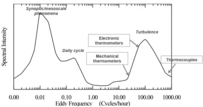
Figure 8. Spectrum of motions in the boundary layer. Regions of
the spectrum are indicated in italics. Arrows point to the highest eddy frequency each type of thermometer can capture (based on a figure of Stull, 1988).
the ground temperature and the two decouple. Finally, when the wind blows stronger, especially during cold advection, it cools down both the 2 m layer and the air near the ground surface at the same time, driving both temperatures towards similar values.
In minimum temperatures, when the vertical gradient stays within ± 1 C m 1, the SLEL2 tends to underestimate
the temperature as compared to the SLMEC with the bias shown in Table 2. When the air above is much cooler than the ground, in general because of cold advection, the two layers decouple and the temperature underestimation by the SLEL2 tends to increase towards higher value.
Contrarily, when a warm advection intervenes, the ground and the air temperature diverge from each other, but electronic thermometers and mechanical thermographs con-verge towards similar values, except for the effect of the Stevenson screen, i.e. about 0.3 C bias.
The author believes that the different response of the two types of thermometers to different boundary layer con-ditions is to be attributed to the weaker ability of mechani-cal thermometers to adjust to temperature variations as com-pared to thermocouples. This coincides with Cheney and Businger (1990), who indicated thermocouples as fast re-sponse thermometers, and with the World Meteorological Organization (WMO, 2008) which suggested that such dif-ferences in time response might become a source of errors.
It has long been known that thermocouple response time is about 1-2 s, thermistors respond in the order of 5 s, bi-metallic thermometers respond in about 20 s and mercury thermometers respond in up to 2-3 minutes, depending on the type of pipe housing the mercury (Stringer, 1972).
However, thermographs usually express temerature at scales of fractions of hours. Electronic data loggers usu-ally average or somehow process sets of row measurements that have been taken within a few seconds from each other, thus smoothing the data to the fraction of minutes. Mercury thermometers are read directly by the observer with no post-processing whatsoever; however, they respond so slowly to
temperature variations that they cannot feel any temperature variations that are faster than a few minutes.
As can be seen in Figure 8 (based on a figure of Stull, 1988), mechanical thermometers are almost unable to cap-ture temperacap-ture variability at the time scale of turbulence. On the other hand, electronic thermometers are actually in-fluenced by the slowest part of such variability, though they cannot properly measure it because they are not designed to fully appreciate turbulence. Since the Tmin and Tmax of an electronic thermometer are the extremes of a set of measure-ments, even one single outlier due to turbulence could change either of them and that would affect the data.
It is clear that whenever turbulent temperature varia-tions are strong, as is the case of the vertical heat fluxes in stable nocturnal boundary layer or the strong vertical heat flux in hot summer daytime, the fast responding elec-tronic thermometers are more likely to catch single outliers in the sets of measurements, thereby causing the general underestimation of Tmin and the summer overestimation of Tmax.
Stull (1988) also pointed out that turbulence of the daily mixed layer is well developed and it has a time scale of 10-15 minutes, while the turbulence of the nocturnal boundary layer is often patchy or discontinuous, so it is much more irregular over space and time. That is the reason why the er-ror in measurements suspected by the World Meteorological Organization (WMO, 2008) is much more likely to occur in minimum temperatures than in maximum ones, as shown by this piece of research.
As far as the effect of wind is concerned, it should be considered that weak winds cause consistent turbulence that is felt by the electronic thermometers. On the other hand, when the wind blows stronger, its steady advection effects become more significant and they are felt by both mechani-cal and electronic thermometers.
The response time of the instruments can also provide an explanation as to why, in calm wind situations, Tmax al-most shows no bias between the SLEL2 and the SLMEC in Figure 7.
In fact, when the wind is calm (less than 0.5 m s 1),
the electronic thermometer stops responding to fast thermal fluctuations, but it is dominated by the slow thermal inertial. Its response time rises to values comparable to those of me-chanical thermometers and that is why they measure much more similar temperatures.
8 Conclusions
The author is aware that the results of this analysis are noisy, so the part of the discussion that deals with the possible causes of the biases could be improved, taking into account the forcings that have not been investigated or improving the tools to analyse the other ones. However, the major impact of the instrumental change is the bias it introduces in long-term climatological studies and, as far as that aspect is concerned, the results given here are indeed quite robust.
Therefore, it is appropriate to suspect that long-term cli-matological analyses of temperature are somehow affected by the change in the measuring technique described in this paper.
Climatologists monitoring minimum and maximum temperatures in climates similar to the one of S. Lucia are likely to encounter a sudden jump in time series around the last decade of the 20thcentury. Considering the topic, this
could be interesting even for other categories of scientists. These results show that precautions should be taken whenever creating time series by merging together tempera-tures registered with mechanical and electronic instruments. In particular, if a single time series or a very small set of them are analysed, typical conditions of the atmospheric boundary layer of the stations locations should be considered, too.
When making separate analyses of winter and summer maximum temperatures in climates similar to this one, it is likely that a negative bias (down to about -1 C) will be found in the former around the end of the 20thcentury and a
posi-tive bias (up to about +1 C) be found in the latter. The two biases, however, would compensate each other if the whole year were considered.
When analysing minimum temperatures, a negative bias of about -0.7 C to -0.8 C (regardless of the season) is likely to be detected in the last decade of the 20thcentury. In order
to cope with that, homogenization must be considered. Finally, considering that many common assessments of global warming are based on long-term analyses of time se-ries of minimum and maximum temperatures combined, the author suspects that in mid-latitude weather stations with cli-mates similar to S. Lucia, the temperature growth in the last two decades could be even greater than what has been esti-mated to date.
Acknowledgements. The meteorological data for this study has been used courtesy of the Department of Agricultural Sciences Unit of Agronomy, Field Crops and Genetics of the University of Sassari and courtesy of the Italian Council for Research in Agriculture Re-search Unit for Climatology and Meteorology applied to Agricul-ture (former UCEA-Ufficio Centrale di Ecologia Agraria) to which the author is grateful for making them available. The author would also like to thank Dr. Giuliano Fois of ARPAS for his support in processing and analysing data and Prof. Maurizio Maugeri of the University of Milan for a critical review of the paper and some very interesting suggestions. The work is partly financed by the Italia-Francia “Marittimo” Operational Programme of the Euro-pean Union, through the RESMAR Project.
References
Brunetti, M., Maugeri, M., and Nanni, T., 2000: Variations of Tem-peratures and Precipitation in Italy from 1866-1995, Theor Appl Climatol,65, 165–174.
Brunetti, M., Maugeri, M., and Nanni, T., 2006: Temperature and precipitation variability in Italy in the last two centuries from homogenised instrumental Time Series, Int J Climatol,26, 345– 381.
Earth Syst Sci,11, 1633–1644.
Peterson, C. P. and Easterling, D. R., 1994: Creation of homoge-neous composite climatological reference series, Int J Climatol, 14, 671–679.
Quayle, R. G., Easterling, D. R., Karl, T. R., and Hughes, P. Y., 1991: Effects of Recent Thermometer Changes in the Coopera-tive Station Network, Bull Amer Meteorol Soc,72, 1718–1723. Simidichiev, D. A., 1986: Compendium of Lecture Notes on
teorological Instruments for Training Class III and Class IV Me-teorological Personnel Volume I. WMO Technical Publication No. 622, World Meteorological Organization, Geneva (CH). Stringer, E. T., 1972: Techniques of Climatology, W.H. Freeman
and Company, San Francisco, CA (USA).
Stull, R. B., 1988: An Introduction to Boundary Layer Meteorol-ogy, Kluwer Academic Publishers, Dordrecht (NL).
Wendland, W. M. and Armstrong, W., 1993: Comparison of Maximum-Minimum Resistance and Liquid-in-Glass Thermome-ter Records, J Atmos Ocean Technol,10, 233–237.
WMO, 2008: Guide to Meteorological Instruments and Methods of Observations. WMO Technical Publication No. 8, World Meteo-rological Organization, Geneva (CH).