Statistical tools for genome-wide studies

(1)

SCUOLA DI DOTTORATO DI RICERCA Scienze e Biotecnologie dei Sistemi Agrari e Forestali e delle Produzioni Alimentari

Scienze e Tecnologie Zootecniche Ciclo XXVI

Anno accademico 2012- 2013

Statistical Tools for Genome-Wide Studies

dr. Massimo Cellesi

Direttore della Scuola prof. Alba Pusino

Referente di Indirizzo prof. Nicolò P. P. Macciotta

Docente Guida dr. Corrado Dimauro

(2)

Massimo Cellesi Statistical Tools for Genomic-Wide Studies

Tesi di Dottorato in Scienze dei Sistemi Agrari e Forestali e delle Produzioni Alimentari Scienze e Tecnologie Zootecniche – Università degli Studi di Sassari

Index

Chapter 1

General Introduction ...6

Pedigree and phenotype to compute EBV ...8

EBV and quantitative trait loci ...9

Genomic Selection ... 10 SNP-BLUP (RR-BLUP) ... 11 G-BLUP ... 12 BAYESIAN METHODS ... 14 BayesA ... 14 Bayesian Lasso ... 16 BayesB ... 17

Genome-wide association studies ... 19

Single marker regression ... 19

The mixed model ... 20

Imputation ... 22

Hidden Markov model ... 23

Outline of the thesis ... 24

References ... 26

Chapter 2 The impact of the rank of marker variance-covariance matrix in principal component evaluation for genomic selection applications ... 31

Summary ... 32

Introduction ... 32

The Principal Component Analysis ... 34

The rank of the genomic variance-covariance S matrix and its effect on PC extraction ... 35

(3)

Materials ... 37

Methods ... 37

Results and discussion ... 38

Conclusions ... 42

References ... 43

Chapter 3 Use of partial least squares regression to impute SNP genotypes in Italian Cattle breeds ... 45

Abstract ... 46 Background ... 46 Methods ... 46 Results ... 46 Conclusions ... 47 Background ... 47 Methods ... 49 Data ... 49

The partial least squares regression imputation method ... 50

Genotype imputation from 3K (7K) LDP to the 50K SNP panel ... 51

Genotype imputation from 3K LDP to the 50K SNP panel for different breeds ... 52

Evaluation of imputation accuracy ... 52

Results ... 53 Discussion ... 56 Conclusions ... 59 Competing interests ... 60 Authors’ contributions ... 60 Acknowledgements ... 60 References ... 61 Chapter 4 Maximum Difference Analysis: a new empirical method for genome-wide association studies ... 65

(4)

Results ... 69 Significant associations ... 69 Milk yield ... 74 Fat yield ... 75 Protein yield ... 76 Fat percentage ... 76 Protein percentage ... 77 Discussion ... 77

Materials and Methods ... 81

The data ... 81

The MDA method ... 81

Conclusions ... 84

References ... 85

Chapter 5 Prediction of direct genomic values by using a restricted pool of SNP selected by maximum difference analysis ... 92

Introduction ... 93

Materials and methods ... 95

The data ... 95

The MDA approach ... 95

Direct genomic value evaluation ... 97

Results ... 98 Discussion ... 99 Conclusion ... 100 References ... 101 Chapter 6 Conclusions ... 103 References ... 107

(5)

(6)

Chapter 1

(7)

Selection in livestock is a technique that has been known for millenniums. In fact, Virgil, in the 3th book of the “Georgica” (36-29 B.C.), wrote about the procedures adopted in bovine selection in his era. Since then, the aim of animal selection has not changed substantially and is generally aimed to obtain animals with high resistance to diseases and high productive performance, both for milk yielded and meat produced. Many years later, Darwin (1869) proposed the use of selection in animal breeding and stated that “The key is man’s power of accumulative selection: nature gives successive variations; man adds them up in certain directions useful to him”.

In any selection procedure, animals have to be evaluated objectively. Therefore, after the traits of interest are individuated, they are studied by using numerical parameters. The first statistical evaluation of the genetic merit of a dairy sire was developed by Lush in 1931. In his work, Lush asserted that the evaluation of an animal was more accurate using a progeny test than a rating based on the pedigree. By using a path coefficient and assuming that genetic and environmental components of variance were known, Lush gave a formula for assessing the genetic merit of dairy sires for factors affecting milk production, using the correlation between the average record of the daughters and the genotype of the sire (Lush 1931). Some years later, Hazel (1943) defined a selection index for measuring the net merit of individuals. To evaluate this index, multiple traits instead of a single trait were taken into account. Using traits of economic importance, an aggregate genotype value for each animal was obtained as a sum of its genotypes weighted by the relative economic value of that trait. Using this aggregate genotype, the selection index was obtained by maximizing the correlation between the aggregate genotype and the index itself, but to get a reliable index a well-estimated phenotype (measured on the animal itself and on its relatives) and a genetic variance-covariance matrix were used.

(8)

The introduction of the selection index was an important milestone in genetic selection because it was the first statistical method used to evaluate the genetic merit of an individual through its phenotype and the phenotypes of its relatives.

Pedigree and phenotype to compute EBV

The estimation of the breeding value (EBV) of animals involved in selection programs is the most important tool to obtain a high genetic improvement in livestock species.

The estimation of breeding value, evaluated by using both pedigree and phenotype recorded on the animals under study, depends on the knowledge of the relationships between the involved individuals. As a consequence, the estimation of the proportion of the phenotypic variance explained to the genotype is obtained by using the relationship matrix. The combination of pedigree and phenotype information with the estimated heritability allows to evaluate the breeding values of the animals. However, due to the enormous dimension of the relationship matrix, a huge amount of computer resources and long computational time are needed (Calus, 2009).

Henderson (1975) proposed a new computational method, named best linear unbiased prediction (BLUP), which is able to improve the accuracy of prediction of breeding values by using all relationships among animals. For many years, this technique has been largely applied and has led to positive results in genetic evaluation programs. However, to get a considerable genetic gain, lots of years are required, especially for traits that can be measured only in one sex (e.g. milk traits), after death (e.g. meat quality) or late in life (e.g. longevity) (Goddard and Hayes, 2009). Another negative aspect of the BLUP approach is that it contributes to an increase in the degree of inbreeding among animals, because it favors the close relatives. Finally, BLUP makes the assumption of the infinitesimal model (Fisher, 1918), where an infinite number of genes with very small effect contribute to the trait (Calus, 2009). This seems a practical but biologically unrealistic assumption because it is known that most of the infinitesimal model assumptions are not verified. Indeed, the number of loci is finite

(9)

or, after repeated selection, the assumption of normality may not be reasonable (Fairfull et al. 2011)

EBV and quantitative trait loci

BLUP and similar statistical procedures, which belong to the so called “quantitative genetics” area, do not use any genetic information directly. The introduction of new molecular techniques able to map the DNA and produce a sparse map of genetic markers has given new momentum to genetic improvement. Fernando and Grossman (1989) applied the BLUP technique to a mixed linear model that also incorporated a marker factor containing information on the linked quantitative trait loci (QTL). Lande and Thompson (1990) showed how molecular genetics could integrate the traditional methods of genetic selection based on phenotypes and pedigree. These methods, where molecular genetics information is integrated in the selection procedures, are known as marker-assisted selection (MAS). This approach was able to increase the genetic gain by 9-38% (Meuwissen and Goddard 1995). With this new approach a more realistic model, alternative to the infinitesimal model, was proposed. In this model, known as the finite locus model, most of phenotype expression is explained by a small number of loci with a large effect, i.e. the QTL, whereas the remaining part of phenotypic variance is explained by a great number of loci with an infinitesimal effect. The initial expectations of a wide use of QTLs in MAS were not completely satisfied because of the presence of some undesirable aspects. Early marker maps were very sparse and, therefore, the QTL mapping was extremely difficult. Associations between chromosome regions and QTLs were studied by using the linkage analysis, which usually locates QTLs at intervals greater than 20 cM. In this scenario, the identification of underlying mutations and the use of marker information in MAS is very difficult (Goddard and Hayes 2009). Nevertheless, some important QTL regions that control milk production were detected in cattle populations (Georges et al. 1995; Weller et al. 1990). However, their use in animal

(10)

breeding programs is not easy, because these models tend to overestimate the QTL effects (Beavis effect) (Xu, 2003b). Moreover, the estimated QTL effects should be validated in an independent population before this information could be used in genetic selection programs. More recent developments in QTL mapping methods have given more precise maps by using the linkage disequilibrium (LD) between markers and QTLs (Aulchenko et al. 2007). The advantage of using the LD for QTL mapping purposes is that the LD quickly decreases as the distance between markers and QTL increases. Consequently, a QTL can be located into a narrower region (Goddard and Hayes 2009). Recently, the availability of high density SNP platforms at reasonably low costs allows to map more and smaller QTLs. Nevertheless, the estimation of QTLs with small effects on the trait under study is difficult and decreases the precision with which the effects of total QTLs are estimated (Calus 2009). Another critical aspect of MAS is that, generally, few markers associated with a QTL are validated in an independent sample population. Using these validated markers, the ability to estimate the breeding value is limited because they explain only a small proportion of the genetic variance. This effect is also confirmed in complex traits studied in humans where only a proportion of the estimated trait hereditability, usually less than half, is explained by QTLs (Stranger et al. 2011).

Genomic Selection

Both accuracy and efficiency of breeding value estimation procedures increased by using the method of Meuwissen et al. (2001), who applied a multiple QTL approach known as genomic selection (GS). This method skipped the QTL-mapping step and estimated the effects of a high number of markers across the genome simultaneously. One of the main difference between the first type of MAS (QTL-MAS) and GS is that QTL-MAS uses the information of a few known QTLs in LD with some markers, whereas GS uses a huge number of markers available in a high density SNP platform. In this approach, all SNPs are considered in LD with a QTL and effects of known and unknown QTLs are accounted for. Furthermore, being all effects simultaneously estimated, the total genetic variance is not, on average, overestimated (Calus 2009; Goddard and Hayes 2009).

(11)

Genomic selection conceptually proceeds in two steps:

• Estimation of the effects of each marker in a reference population where genotypes

and a reliable EBV are known;

• Prediction of the genomic estimated breeding values (GEBV) for animals not present

in the reference population, such as young selection candidates, with known genotypes but without performance records.

In the second step, GEBVs of animals with genotype data but not phenotypes are estimated by summing the effect of each marker across the whole genome:

ˆ GEBV Xg=

where X is a design matrix allocating animals to genotypes, and ˆgis the vector of marker

effects.

There are, however, two main critical issues in the estimation of marker effects. The first is that the number of marker effects that have to be estimated is greater than the number of animals with known genotype and phenotype. The second regards the assumption related to the prior distribution of the variance of SNP effects. Some of the models proposed to solve these problems are the SNP-BLUP (Meuwissen et al. 2001; Moser et al. 2010), the GBLUP (Hayes et al. 2009, Van Raden et al. 2009) and the Bayesian approach termed as Bayes-alphabet (Meuwissen et al. 2001; Xu 2003a). Each model makes different assumptions about the prior distribution of marker effects.

SNP-BLUP (RR-BLUP)

The SNP-BLUP (RR-BLUP) model assumes that each of m SNP has a very small effect on the genetic variance of the trait. If n is the number of animals with known genotype and reliable EBV and m is the number of markers, the model is:

(12)

1_n

y= µ+Xg e+

where y is the reliable EBV, 1_nis a vector of 1s, µ is the overall mean, X is a design matrix,

allocating records to genotypes for markers (n rows and m columns), g is a vector of random

effect of markers, and e is a vector of residuals that are assumed to be normally distributed

with

(

_0, 2

)

e

e N Iσ . In this model marker effects are assumed to be normally distributed

with

(

_0, 2

)

g

g N Iσ , where 2

g

σ is the variance of the marker effects. The solution of the

previous model is given by:

1 ˆ 1 1 1 1 ˆ 1 n n n n n X y X X X I g X y µ λ − ′ ′ ′       =       _′ _′ ₊ _′       where e2₂ g σ λ σ

= and I is the identical matrix. 2

g

σ is unknown but can be calculated from the

total genetic additive variance 2

a

σ , estimated, for instance, by REML (Gilmour et al. 2009).

Therefore, assuming that all markers contribute equally to the total amount of the explained

variance, the genetic variance can be estimated as 2 a2

g _m

σ

σ = . This assumption, however,

seems unrealistic (Meuwissen et al. 2001). A more accurate estimation of 2

g

σ can be done by

taking into account the differences in marker allele frequencies as follows:

(

)

2 2 1 2 1 a g m j j j p p σ σ = = −

∑

where pjis the allele frequency of marker j.

G-BLUP

An alternative and equivalent method to the SNP-BLUP, to estimate GEBV using marker information, is the G-BLUP, which uses a genomic relationship matrix G instead of the pedigree derived relationship matrix (Van Raden 2008, Hayes et al. 2009). Moreover, in the

(13)

G-BLUP, the genetic variance explained by each marker is not constant and changes according to marker allele frequencies. The G-BLUP model is:

1_n

y= µ+Zg e+

where y is the reliable EBV, 1nis a vector of 1s, µ is the overall mean, Z is a design matrix

allocating records to breeding values, g is the vector of SNP effects, and e is a vector of

random residuals, which are assumed to be normally distributed with

(

_0, 2

)

e

e N Iσ . Let

g Wu= where u is the a vector of breeding values and _i _{( )} 2

u

Var g WW= ′

σ

where 2

u

σ is the variance breeding values. W is a design matrix allocating records to genotypes with

, , 2

i j i j j

w =x − p , where x_{,i j}is the genotype jth SNP of the ith_{animal and p}

j is the allele

frequency of jth markers. If WW ′is scaled, the genomic relationship matrix G is defined as

, 1 n i i i nWW G w = ′ =

∑

and 2 ( ) _g

Var g =Gσ . Using this model, the breeding value for both phenotype and non-phenotype individuals can be evaluated by the equations as follows:

1 2 1 2 1 1 1 ˆ 1 1 ˆ n n n n e n g Z y Z Z Z G g Z y µ σ σ − − ′ ′   ′     ₌       _′ _{′ +}  _′   _ _    

This method is very attractive for populations without good pedigree records because the genomic relationship matrix will capture this information among the genotyped individuals. The accuracy of the estimation of GEBV in single breed populations of G-BLUP agrees reasonably well with the accuracy achieved with other methods such as BayesA. When the animals in the reference and validation sets are in a multi-breed population, the accuracy of G-BLUP is lower than that of BayesA (Hayes et al. 2009).

(14)

BAYESIAN METHODS

Both G-BLUP and SNP-BLUP approaches assume that all SNP effects are non-zero, small and

normally distributed. Moreover, the two methods evaluate the genetic variance 2

g

σ from the

additive variance 2

a

σ . Under these assumptions, the vector of marker effects ˆg can be easily

estimated and consequently the GEBV of animals can be calculated. With different and more realistic assumptions about the variance explained by each locus or about the prior distribution of marker effects, the GEBV prediction could be more accurate. However, the

evaluation of the genetic effects ˆg is more complicated and requires complex statistical

tools.

BayesA

The BayesA is an alternative method to BLUP to estimate the EBV. In this method data are modeled at two levels. The first model is developed at the level of the SNP and is similar to the SNP-BLUP model. The second model is developed at the level of variance across the SNPs.

The first model is:

1n

y= µ+Xg e₊

_0, 2

)

i

i g

g _N σ . The latter distribution highlights that the variance of each

effect is not constant as in SNP-BLUP. This assumption seems to be more realistic. Indeed, if

the variability of the variance that affects the effect ˆg , i σg2i, is large then ˆg can be large, i

whereas if 2

i

g

σ is small, then the effect ˆg decreases towards zero. This model, termed as i

BayesA, can be solved as:

1 1 1 2 1 2 1 1 2 2 1 1 1 . 1 ˆ ₁ _. 1 ˆ . . . . ˆ 1 . m n n n n m e n n g m e m m n g X X y X X X I X X g X y g X y X X X X X I σ µ σ σ σ − ′ ′ ′     _′      _′ _′ ₊ _′        _′     =              _′   _ _′ _′ _{′ +} _       .

The second model, considered at the level of variances of SNP effects, allows to evaluate the

2

i

g

σ for each SNP. The variance of effects is evaluated recursively. In the first step the prior

distribution of 2

e

σ and the prior distribution of 2

i

g

σ are fixed. After, the posterior distribution

of effects across all the genome and the posterior distribution of the overall mean are

evaluated. The prior distribution of error variance 2

e

σ is chosen as _χ−2

( )

_2,0 _{because it gives}

an uninformative and uniform prior distribution. With these assumptions, the conditional posterior distribution of error variance is:

( )

_,

i

g

ior σ ₌χ− v S _{where v is the number of}

(16)

useful because, by combining it with the normal distribution of data, the posterior

distribution of 2

i

g

σ also becomes a scaled inverted chi-squared:

( )

2 2

( )

Prior σg_i =χ− v S, → Post

(

σg2i |gi

)

χ 2

(

v n S g gi, i i

)

− _′

= + +

where ni is either the number of haplotype effects at segment i or 1 when a single effect is

estimated for each SNP. Meuwissen et al. (2001) fixed v and S as v = 4.012 and S = 0.002 to get a distribution similar to that of QTL effects obtained by Hayes and Goddard (2001) and to obtain the expected heterozygosity of QTL when the neutral model is considered (Hayes and

Daetwyler 2013). Xu (2003a) proposed 2

1

χ− _{(with 1 d.f.), whereas Ter Braak et al. (2005)}

proposed 2

0.998

χ− _(with_{1 2}₋ _δ_{d.f.). As shown above, the posterior distribution of variance}

effects depends on the knowledge of the effect giand, therefore, σg2i cannot be directly

estimated. Likewise, gi depends on σg2_i. This problem can be solved using the Gibbs sampling

to estimate effects and variances. The Gibbs sampler runs many times (more than 10,000

cycles) for each SNP and, once the first hundreds of evaluations of giare discarded, the final

effect of the ith_{SNP, ˆ}

i

g , is obtained as the average of the remaining evaluations of gi. The

combination of the assumptions of normality distribution of marker effects and inverted chi-squared distribution of variance effects results in a t-distribution of the posterior conditional distribution of marker effects, where the probability of getting SNPs with moderate or large effects is greater than in a normal distribution.

Bayesian Lasso

Bayesian Lasso (BayesL) (Xu 2003a; Yi and Xu 2008) is similar to the BayesA approach. BayesL uses the same model and the same procedure of BayesA to evaluate marker effects, but it makes a different assumption about the distribution of markers variance. In BayesL,

( )

2

(17)

posterior distribution of SNP effects ˆgresults in a double-exponential expression.

Double-exponential distribution has a larger peak at zero and heavier tails than the normal distribution. As a consequence, the effects of a large number of markers will be very close to zero.

BayesB

Another possible assumption about the distribution of marker effects is a situation where a lot of SNPs are located in regions with no QTL and, consequently, have zero, whereas some SNPs have a moderate or large effect because they are in linkage disequilibrium with QTLs. Meuwissen et al. (2001) called this method BayesB and proposed a prior distribution of marker effects where many SNPs have zero effects whereas the remaining markers have a

normal distribution. In BayesB, the prior distribution is fixed with a high density, π, at 2 ₀

i

g

σ =

and with an inverse chi-square distribution at 2 ₀

i g σ > : 2 ₀ i g σ = with probability π

( )

2 2 _, i g v S σ ₌χ− _{with probability (1- π),}

where v = 4.234 and S = 0.0429 (Meuwissen et al. 2001). The Gibbs sampler described in

BayesA cannot be used in the BayesB method, because it moves only where 2 ₀

i

g

σ > . Indeed,

if g ≠i 0, it is not possible to sample from a distribution with σ2gi = , whereas the 0

probability of finding g =i 0 is infinitesimal when σg2i > . This problem was solved by 0

sampling 2

i

g

σ and gi simultaneously using a Metropolis-Hastings algorithm (Meuwissen et

al. 2001).

Even if there are many works where Bayesian methods yield a more accurate prediction of GEBV than SNP-BLUP, these results are often obtained using simulated published data (Meuwissen et al. 2001; Habier et al. 2007). However, when using real data, the best

(18)

performances of Bayesian methods are not consistently verified. One reason for the disagreement observed between real and simulated data could be differences between the genetic architecture of the real population and that of simulated data. It is well known that

accuracy is proportional to hereditability (h2) and to the number of individuals in train

population (Np). Daetwyler et al. (2010) demonstrated that the accuracy of SNP-BLUP, for a

given Np and h2, was not dependent on the number of QTL (NQTL), whereas the accuracy of

BayesB was high when NQTL was low but it decreased when NQTL increased. In addition,

sometimes, the accuracy of SNP-BLUP was higher than the accuracy of BayesB when NQTL was

high.

Another problem that affects both BayesA and BayesB is their sensitivity to the prior distribution and the parameter specification. In a simulated dataset, Lehermeier et al. (2013) tested the sensitivity of four Bayesian methods frequently used in genome-based prediction: Bayesian Ridge, BayesL, BayesA and BayesB. The authors found that the predictive abilities of the tested Bayesian methods were similar, but the performances of BayesA and BayesB depended substantially on the choice of parameters. However, all Bayesian approaches require huge computer resources and are time expensive (Shepherd et al. 2010). The reason is that Markov Chain Monte Carlo techniques, such as Gibbs sampling and Metropolis-Hasting algorithm, require thousands of samplings to detect the effect of each SNP. If the data dimension is small, these techniques are feasible. However, in genomic selection, animals are genotyped by using high density SNP platforms and, in this case, a huge computational time is needed.

Several other methods have been proposed to predict the genomic breeding values of animals in selection programs. Apart from few approaches which assume an equal contribution of all loci to the genetic variance, a common challenge of the most part of these methods is to reduce the dimensionality of the SNP data (Calus 2009). The reduction of the number of SNP involved in genomic evaluations brings down the genotyping costs and might reduce the bias due to SNP that are not in LD with any QTL.

(19)

Genome-wide association studies

Genome-wide association studies (GWAS) is a way to detect associations between markers and production or functional traits or diseases. Associations are studied by examining many common genetic variants in different individuals and then verifying if any variant is associated with a trait of interest. In animal breeding programs, knowledge of the genes that affect a particular trait can be used to select animals carrying desirable alleles (Goddard and Hayes, 2009; Ron and Weller, 2007; Wiener et al. 2011). There are many approaches to implement GWAS for quantitative traits, and the simplest one is the use of a linear regression for each marker.

Single marker regression

Under the assumption of random mating among animals with no population structure, the association between SNPs and traits can be tested by using the following model:

y Wb Xg e= + +

where y is the trait, W is a design matrix for fixed effects (e.g. mean, age and season of birth),

b is the vector of fixed effects, X is the vector of the SNP genotypes, g is the effect of the

markers, and e is the vector of residuals, assumed to be normally distributed with mean zero

and variance 2

e

σ :

(

_0, 2

)

e

e N_ σ . In this model the effect of each marker is additive and is

considered as a fixed effect. The null hypothesis H0 is that the marker has no effect on the

trait, whereas the alternative hypothesis H1 is that the marker is in LD with a QTL that affects

the trait. The statistical test used to test the H0 is a F-test and H0 is rejected if F F> α, ,n m

where α is the level of significance and n and m are the degrees of freedom. The choice of the level α of significance is a crucial point in GWAS. In genomic data analyses, tens of thousands of markers are tested and, therefore, the α value of 0.05 normally used leads to a

(20)

very high number of false positive associations. For example, the 50K Illumina’s chip contains around 50,000 SNP. If a threshold is fixed, the expected false positive associations are

50,000 0.05 2,500× = . To overcome this problem, a correction for the multiple test error can be applied. Usually, the Bonferroni correction is adopted, but it is extremely conservative and discards most of possible true associations. In fact, referring to the previous example, the

threshold that should be fixed with the Bonferroni correction is 0.05 ₁₀ 6

50,000

α ₌ ₌ − _{and this}

value would probably cut off most associations. An alternative empirical procedure is the

permutation test (Churchill and Doerge, 1994), which is an excellent method for setting significance thresholds in a random mating population. On the other hand, the permutation test takes a lot of time because it fixes the α threshold by randomly shuffling, for each marker, the phenotypes across individuals thousands of times.

Another source of spurious associations is the stratification of the population due to the genetic drift or to the artificial selection that exists in some livestock populations (Ma et al., 2012). These effects can be removed by using a mixed model with the population structure as random effect.

The mixed model

In mixed models, the expectation of the outcome y is modeled using both fixed and random effects. Fixed effects are the same as those of the single marker regression, whereas random effects are the polygenic effect due to population structure. In cattle breeds, the assumption of independence between traits does not hold because relatives in the sample population

share genomes and the traits are controlled by genome. The heritability h2 characterizes the

strength of control of the trait by genome, whereas the coefficient of relationship φ,i j, which

characterizes the relationship between a couple of relatives i and j, is roughly proportional to the genome shared identical-by-descent. Correlations among phenotypes of the relatives i

(21)

evaluated by the relation 2

, ,

i j h i j

ρ = φ . The model which takes into account the correlation

structure is the following:

1_n

y= µ+bX Za e+ +

where y is the vector of reliable EBV, 1_n is a vector of 1s, µ is the overall mean, X is the

vector of the considered SNP genotype, b is the regression coefficient, Z is a design matrix for

animal effects, a is the vector of the random additive polygenic effects with _(0, 2₎

a

a N_ Φσ ,

where Φ =

{ }

ρ,ih is the additive genetic relationship matrix, and e random residual effect

with _(0, 2₎

e

e N Iσ (Yu et al. 2006, Aulchenko et al. 2007). The structure of the mixed model

is like that of BLUP and, therefore, its solutions are obtained as previously described for the BLUP model. The significance of the regression coefficient b and consequently the associations between SNPs and traits are assessed by using a t-test or Wald chi-squared. Even if the mixed model solves the problem of the population stratification, it still has the shortcomings of multiple testing. When a single-marker linear regression is used to test associations for complex traits, the model might lead to inconsistent estimation of marker effects because markers are in linkage disequilibrium with many QTL (de Los Campos et al. 2010). In animal breeding, most of the productive traits are affected by a large number of genes with possible interactions among them. As a consequence, in genetic studies of complex traits, the single-locus analysis does not produce reliable results (Cordell, 2009). Another disadvantage of the single SNP approach is that LD could extend to a wide genome region. In this case, the detection of the region containing the true mutation and the significant associated SNPs could be difficult (Pryce et al. 2010). A possible solution to this problem could be to fit all SNPs simultaneously by using the Bayesian-alphabet model.

Whatever the method used for GWAS, SNPs declared associated with a trait have to be validated, even if a stringent threshold is used to detect the statistical associations. The best way to validate the detected SNPs is to verify the associations in an independent population. In livestock, where the degree of inbreeding is high and the pedigree structure could affect

(22)

independent samples, the most convincing validation method is across breeds. However, if a SNP does not segregate in the breeds considered in the validation procedure, the validation of the SNP across breeds might fail.

Imputation

Genotype imputation indicates the process of predicting genotypes that are not directly assayed from a SNP chip panel. These “in silico” genotypes can be used to boost the number of SNPs across the whole genome as part of a GWAS or a GS program. The imputed markers can be also used in a more focused region as part of a fine-mapping study (Marchini and Howie 2010). In GWAS and GS, high-density marker panels of different SNP densities (50K and 777K) are currently used to genotype bulls and elite cows under study (Hayes et al. 2009, Schopen et al. 2011, Chamberlain et al. 2012). In animal science, genotyping costs are one of the major constraints which limit a large-scale implementation of GS. However, the commercial availability of low-density SNP panels has offered new opportunities to increase the number of animals involved in association studies and, above all, in selection programs. Genotypes obtained from a low-density panel are currently imputed to a high-density chip and used in addition to genotypes obtained with a high density panel.

Imputation is very useful when genotypes coming from different chips panel have to be joined (Druet et al 2010). In this case, imputation can increase the sample size of the population under study. In GWAS this implies an increase in the power of a given study and can also facilitate meta-analyses in studies that combine genotypes obtained from different sets of variants (Howie et al. 2011).

The Hidden Markov Model (HMM) is the most useful approach to perform imputation. It is used in many of the available software suite programs, such as Beagle (Browning and Browning 2009), IMPUTE2 (Howie et al. 2009) and FastPHASE (Scheet and Stephens 2006).

(23)

Hidden Markov model

HMM are probabilistic models where the resulting sequences are generated by two concurrent stochastic processes. The first is a one-state Markov model where the probability of transition from state j-1 to state j depends only on state j-1. In the second process, there is the emission of a value (the haplotypes or the genotypes) which is regulated by an emission probability depending on the state. The result is a sample of sequences conditioned by the transition between states (i.e. ACCGTC). Because only the final sequence can be observed, with no understanding of the Markov process, the model is termed hidden.

Figure 1 A Hidden Markov model for DNA sequences. The circled Si are the hidden states and the arrows

between the states indicate the state-transition probabilities. Letters inside squares indicate the symbols of emission and the arrows between a state and a symbol are the emission probabilities.

Using Rabiner’s notation (Rabiner 1989), the five components of a HMM are as follows:

• N hidden states: S1, S2, …. , SN;

• M different symbols (the haplotypes A C G T): v1, v2, …. , vM;

• State-transition probabilities A a={ }i j, : ai j, =P x

(

t =S xj| t−1=Si

)

that is the

(24)

• Emission probabilities B={ }bj k_, : the probability of observing the symbol vk in the

state Sj;

• Initial-state probabilities distribution π ={ }πi : πi =P x S

(

1= i

)

that is the probability

that the HMM process starts at state Si.

In Figure 1 there is a HMM for DNA sequences with the Rabiner’s notation.

Once parameters N and M are fixed, the model is described by means of λ={ , , }A B π , which

is obtained fixing suitable values for A, B and π. Several problems arise with a HMM

inferring the probability of an observed sequence or detecting which could be the most likely sequence. If the entire sequence s of length L generated by the HMM is known and if w is the path of the starting state till the final state, the joint probability to observe s is:

(

)

0,1 , 1 , 1 , | L t t t k t P s w λ a a ₊ b =

=

∏

. Being w unknown, all possible paths should be considered and,

consequently, the probability to observe the sequence s is

(

|

)

(

, |

)

w

P s λ =

∑

P s w λ . The procedure to evaluate s is computationally expensive, even for simple applications. To solve this problem, the forward-backward algorithm was proposed (Baum and Egon 1967; Baum 1972). This algorithm reduces the number of paths to be considered and, consequently, the probability of sequence s can be determined. Once the sequence is fixed, the next step is to detect the most probable state sequence that generated it. This issue can be efficiently solved by using the Viterbi algorithm (Viterbi 1967).

In conclusion, an important shortcoming of the methods based on HMMC is that all of them require a very long computation time.

Outline of the thesis

The overall aim of this thesis is to propose some alternative approaches to evaluate the genomic breeding value of animals involved in genomic selection programs. Moreover, a new

(25)

method to develop genome wide association studies is proposed. This new method was also used to reduce the dimensionality of the SNP data. These selected SNPs were then used to estimate the breeding values.

(26)

References

• Aulchenko YS, de Koning J, Haley C (2007) Genomewide rapid association using mixed

model and regression: a fast and simple method for genomewide pedigree–based quantitative trait loci association analysis. Genetics, 177: 577–585.

• Balding DL (2006) A tutorial on statistical methods for population association studies.

Nature Reviews Genetics, 7: 781–79

• Baum L (1972) An equality and associated maximization technique in statistical

estimation for probabilistic functions of Markov processes. Inequalities, 3: 1–8.

• Baum L, Egon JA (1967) An equality with applications to statistical estimation for

probabilistic functions of a markov process and to a model of ecology. B Am Math Soc, 73: 360–363.

• Browning BL, Browning SR (2009) A unified approach to genotype imputation and

haplotype–phase inference for large data sets of trios and unrelated individuals. Am J Hum Genet, 84: 210–23.

• Calus MPL (2009) Genomic breeding value prediction: methods and procedures.

Animal, 4: 157–164.

• Chamberlain AJ, Hayes BJ, Savin K, Bolormaa S, McPartlan HC, Bowman PJ, Van Der

Jagt C, MacEachern S, Goddard ME (2012) Validation of single nucleotide polymorphisms associated with milk production traits in dairy cattle. J Dairy Sci, 95: 864–875.

• Churchill GA, Doerg RW (1994) Empirical threshold values for quantitative trait

mapping. Genetics, 138: 963–971.

• Cordell HJ (2009) Detecting gene–gene interactions that underlie human diseases.

Nat Rev Genet, 10: 392–404.

• Daetwyler DH, Pong–Wong R, Villaneuva B, Woolliams JA (2010) The impact of

genetic architecture on Genome–Wide evaluation methods. Genetics, 185: 1021– 1031.

(27)

• Darwin CR (1869) On the origin of species by means of natural selection, or the

preservation of favoured races in the struggle for life. London: John Murray.

• de Los Campos G, Gianola D, Allison DB (2010) Predicting genetic predisposition in

humans: The promise of whole–genome markers. Nat Rev Genet, 11: 880–886

• Druet T, Schrooten C, de Roos APW (2010): Imputation of genotypes from different

single nucleotide polymorphism panels in dairy cattle. J Dairy Sci, 93: 5443–5454.

• Fairfull RW, McMillan I, Muir WM (1998) Poultry Breeding: Progress and prospects for

genetic improvement of egg and meat production. In Proceedings of the 6th World Congress on Genetics Applied to Livestock Production–WCGALP, Armidale, Australia, pp. 271–278.

• Fernando RL, Grossman M (1989) Marker assisted selection using best linear unbiased

prediction. Genet Sel Evol, 21: 467–477.

• Fisher R (1918) The correlation between relatives on the supposition of Mendelian

inheritance. Trans Roy Soc Edin, 52: 399–433.

• Georges M, Nielsen D, Mackinnon M et al. (1995) Mapping Quantitative Trait Loci

Controlling Milk Production in Dairy Cattle by Exploiting Progeny Testing. Genetics, 139: 907–920.

• Gilmour AR, Gogel BJ, Cullis BR, Thompson R (2009). ASReml user guide release 3.0.

VSN International Ltd, Hemel Hempstead, UK.

• Goddard ME and Hayes BJ (2009) Mapping genes for complex traits in domestic

animals and their use in breeding programmes. Nat Rev Genet, 10: 381–391.

• Habier D, Fernando RL, Dekkers JCM (2007) The impact of genetic relationship

information on genome–assisted breeding values. Genetics, 177: 2389–239.

• Hayes BJ, Bowman PJ, Chamberlain AJ, Goddard ME (2009): Genomic selection in

dairy cattle: progress and challenges. J Dairy Sci, 92: 433–443.

• Hayes BJ, Daetwyler H (2013) Genomic Selection in the era of Genome sequencing.

(28)

• Hayes BJ, Goddard M.E. (2001) The distribution of the effects of genes affecting

quantitative traits in livestock. Genet Sel Evol, 33: 209–29.

• Hazel LN (1943) The genetic basis for constructing selection index. Genetics 28: 476–

490.

• Henderson CR (1975) Rapid method for computing inverse of a relationship matrix. J

Dairy Sci, 58: 1727–1730.

• Howie B, Marchini J, Stephens M (2011) Genotype Imputation with Thousands of

Genomes. G3 (Bethesda), 1: 457–470.

• Howie BN, Donnelly P, Marchini J (2009) A flexible and accurate genotype imputation

method for the next generation of genome–wide association studies. PLoS Genet, 5: e1000529.

• Lande R, Thompson R (1990) Efficiency of marker–assisted selection in the

improvement of quantitative traits. Genetics, 124: 743–756.

• Lehermeier C, Wimmer V, Albrecht T, Auinger HJ, Gianola D, Schmid VJ, Schön CC

(2013). Sensitivity to prior specification in Bayesian genome–based prediction models. Stat Appl Genet Mol Biol, 1–17.

• Lush JL (1931) The number of daughters necessary to prove a sire. J Dairy Sci, 14:

209–220.

• Ma L, Wiggans GR, Wang S, Sonstegard TS, Yang J et al. (2012) Effect of sample

stratification on dairy GWAS results. BMC Genomics, 13: 536.

• Marchini J, Howie B (2010) Genotype imputation for genome–wide association

studies. Nat Rev Genet, 11: 499–511.

• Meuwissen THE, Goddard ME (1996) The use of marker haplotypes in animal

breeding scheme. Genet Sel Evol, 28: 161–176.

• Meuwissen THE, Hayes BJ, Goddard ME (2001) Prediction of total genetic value using

(29)

• Moser G, Khatkar MS, Hayes BJ, Raadsma HW (2010) Accuracy of direct genomic

values in Holstein bulls and cows using subsets of SNP markers. Genet Sel Evol, 42: 37.

• Pryce JE, Bolormaa S, Chamberlain AJ, Bowman PJ, Savin K, Goddard ME, Hayes BJ

(2010) A validated genome–wide association study in 2 dairy cattle breeds for milk production and fertility traits using variable length haplotypes. J Dairy Sci, 93: 3331– 45.

• Rabiner LR (1989). A tutorial on hidden Markov models and selected applications in

speech recognition. Proc IEEE Inst Electr Electon Eng, 77: 257–286.

• Ron M, Weller JI (2007) From QTL to QTN identification in livestock –winning by

points rather than knock–out: a review. Anim Genet, 38: 429–439.

• Scheet P, Stephens M (2006) A fast and flexible statistical model for large–scale

population genotype data: Applications to inferring missing genotypes and haplotypic phase. Am J Hum Genet, 78: 629–44.

• Schopen GCB, Visker MHPW, Koks PD, Mullaart E, van Aredonk JAM, Bovenhuis H

(2011): Whole–genome association study for milk protein composition in dairy cattle. J Dairy Sci, 94: 3148–3158.

• Shepherd R, Meuwissen T, Woolliams J (2010). Genomic selection and complex trait

prediction using a fast EM algorithm applied to genome–wide markers. BMC Bioinformatics, 11: 529.

• Stephens M, Balding DJ (2009). Bayesian statistical methods for genetic association

studies. Nat Rev Genet, 10: 681–690.

• Stranger BE, Stahl EA, Raj T (2011) Progress and promise of genome–wide association

studies for human complex trait genetics. Genetics, 187: 367–383.

• Ter Braak CJF, Boer MP, Bink MCAM (2005) Extending Xu's Bayesian model for

estimating polygenic effects using markers of the entire genome. Genetics, 170: 1435–1438.

(30)

• Van Raden PM (2008) Efficient Methods to Compute Genomic Predictions. J Dairy Sci,

91: 4414–4423.

• Van Raden PM, Van Tassell CP, Wiggans GR, Sonstengard TS, Schnabel RD, Taylor JF,

Schenkel FS (2009) Invited review: reliability of genomic predictions for North American Holstein bulls. J Dairy Sci, 92: 4414–4423.

• Viterbi A. (1967) Error bounds for convolutional codes and an asymptotically

optimum decoding algorithm. IEEE T Inform Theory, 13: 260–269.

• Weller JL, Kashi Y, Soller M (1990) Power of daughter and granddaughter designs for

determining linkage between marker loci and quantitative trait loci in dairy cattle. J Dairy Sci, 73: 2525–2537.

• Wiener P, Edriss MA, Williams JL, Waddington D, Law A, Woolliams JA, Gutiérrez–Gil B

(2011) Information content in genome–wide scans: concordance between patterns of genetic differentiation and linkage mapping associations. BMC Genomics, 12: 65.

• Xu S (2003a) Estimating polygenic effects using markers of the entire genome.

Genetics 163:789–801.

• Xu S (2003b) Theoretical Basis of the Beavis Effect. Genetics, 165: 2259–2268.

• Yi N, Xu S (2008) Bayesian LASSO for quantitative trait loci mapping. Genetics, 179:

1045–1055.

• Yu J, Pressoir G, Briggs WH, Vroh Bi I, Yamasaki M, Doebley JF, McMullen MD, Gaut

BS, Nielsen DM, Holland JB, Kresovich S, Buckler ES. (2006). A unified mixed–model method for association mapping that accounts for multiple levels of relatedness. Nat Genet, 38: 203–208.

(31)

Chapter 2 The impact of the rank of marker

variance-covariance matrix in principal component

evaluation for genomic selection applications

Corrado Dimauro, Massimo Cellesi, Maria Annunziata Pintus, Nicolò P.P. Macciotta

Dipartimento di Scienze Zootecniche, Università di Sassari, via De Nicola 9, 07100 Sassari, Italy

Published in Journal of Animal Breeding and Genetics (2011) 128: 440-445.

(32)

Summary

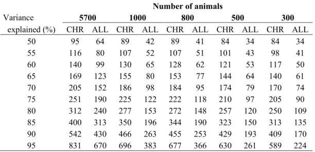
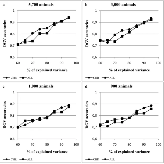
In genomic selection (GS) programs, direct genomic values (DGV) are evaluated by using information provided by high-density SNP chip. Being DGV accuracy strictly dependent on SNP density, it is likely that an increase of the number of markers per chip will result in severe computational consequences. Aim of present work was to test the effectiveness of principal component analysis (PCA) carried out by chromosome in reducing the marker dimensionality for GS purposes. A simulated data set of 5,700 individuals with an equal number of SNP distributed over 6 chromosomes was used. PCs were extracted both genome-wide (ALL) and separately by chromosome (CHR) and used to predict DGVs. In the ALL scenario, the SNP variance-covariance matrix (S) was singular, positive semi-definite and contained null information which introduces ‘spuriousness’ in the derived results. On the contrary, the S matrix for each chromosome (CHR scenario) had a full rank. Obtained DGV accuracies were always better for CHR than ALL. Moreover, in the latter scenario DGV accuracies became soon unsettled as the number of animals decreases whereas, in CHR, they remain stable till 900-1,000 individuals. In real applications where a 54K SNP chip is used, the largest number of markers per chromosome is about 2,500. Thus a number of around 3,000 genotyped animals could lead to reliable results when the original SNP-variables are replaced by a reduced number of PCs.

Introduction

In the last decade, several countries have developed breeding programs based on genomic selection (GS). In this approach, the genetic merit of an animal is assessed by using marker information provided by dense SNP platforms (Fernando et al. 2007). The BovineSNP50 BeadChip (Illumina Inc., San Diego, CA), which contains 54K SNP-markers, has been the most used platform in bovine genomic studies. It is likely that SNP chip density will be further enlarged in the very next future, being direct genomic value (DGV) accuracy strictly

(33)

dependent on SNP density (Solberg et al. 2008). Recently, a 777K SNP platform has been made available (Illumina Inc., San Diego, CA) for bovine genotyping. In human genetics, for example, over one million SNPs are usually typed per individual (Hinds et al. 2005; The International Hapmap Consortium 2005). However, expertise is hardly transferable to animals being genomic information, in human genetics, mainly used for association studies. In genomic selection, the primary aim of animal genotyping is the estimation of DGV which is highly computational demanding. Moreover, being DGV accuracy strictly dependent on the number of animals with genotypes and phenotypes available (i.e. size of the reference population), a large number of individuals has to be genotyped, thus increasing the amount of data to be processed. As an example, a data matrix (X) of nearly 4 billion columns is generated if 5,000 animals are genotyped with the 777K chip. Such amount of records is very difficult to handle and the use of complex algorithms such as BLUP, Bayes A (Meuwissen et al. 2001) or LASSO (Park & Casella 2008) requires a huge computational capacity. Therefore, the search for methods able to reduce the dimension of the X matrix represents a priority. With this aim, Vazquez et al. (2011) proposed to select relevant SNP by single marker regression on phenotypes. However, results on actual data highlight a reduction of DGV accuracy when a number of SNP are deleted. Moreover, being SNP selection based on their relevance on the analyzed phenotype, specific sets of SNP should be needed for different traits (Habier et al. 2009).

Actually, the deletion of some columns in the data matrix X should be avoided, considering the great economic effort for genotyping a large number of animals with the highest marker density available. A more rational approach should summarize information contained on the whole SNP panel in a smaller set of new variables. This is the case of the principal component analysis (PCA) (Hotelling 1933). This technique removes any redundancy in the original data by searching for a new set of mutually orthogonal variables (the principal components, PC), each accounting for decreasing amount of variance in the data. PCA has been used to analyze human genetic patterns (Cavalli Sforza & Feldman 2003; Paschou et al. 2007). Recently, Lewis et al. (2011) applied PCA to a genomic dataset (30,000 SNP) generated in a study

(34)

involving 19 breeds (13 taurine, three zebu, and three hybrid breeds). Authors demonstrated that 250-500 carefully selected SNP are sufficient to trace the breed of unknown cattle samples. In GS simulated experiments, PCA has been used to reduce the dimension of the SNP data matrix for DGV prediction (Macciotta et al., 2010; Solberg et al., 2009), obtaining similar accuracies when either SNPs or PCs were used as predictors. These results indicate that PCA can be considered a suitable tool to reduce the number of SNP variables in GS programs.

Aim of this work was to demonstrate, both in theory and in practice, that a proper use of PCA may be effective in reducing the marker dimensionality for GS purposes.

The Principal Component Analysis

PCA is a statistical procedure that transforms a number of (possibly) correlated variables into an equal number of uncorrelated variables called PCs. The objective of PCA is to redistribute the original variability of data. Thus, the first principal component accounts for as much as possible of original variability in the data, and all components are extracted in order to maximize successively the amount of variance explained (Morrison 1976; Krzanowsky 2003). In other words, to summarize information contained in the starting m-dimensional space (the m SNP-variables), original directions are rotated into a new m-dimensional space. The new m-directions are the principal components where the jth PC is represented by a linear

combination of the observed variables Xm:

1 1 ...

j j mj m

PC =v X + +v X

with j=1,……,m. The vmj weights are the components of the eigenvectors extracted from the

variance-covariance (correlation) matrix (S) in a so called “eigenvalue problem”. The S matrix is symmetric and positively semi-definite. It has on the diagonal the variances of each m-variable and off diagonal the covariance between m-variables. The trace of S (trS) represents

(35)

the total variance of the multivariate system. The eigenvalue problem applied to S gives the following results: i) m eigenvalues, λ1> λ2>………> λm ≥0, such as m i i trS λ =

∑

.

ii) a set of m vectors (eigenvectors), one for each eigenvalue. These vectors are mutually

orthogonal and their components are the weights vmj used to compose the PCs. These

vectors constitute the matrix V of the eigenvectors.

The first eigenvalue is greater than the second, the second is greater of the third and so on.

The proportion of the total variance accounted by the ith component (varexpl) can be

empirically evaluated as:

expl var i

trS

λ

=

Finally, the matrix P whose columns are the new variables, can be calculated as:

P X V= ⋅ whose dimension is (nxm).

One crucial step of PCA concerns the choice of the number of PCs to be retained. Several methods have been proposed (see Jolliffe, 2002, for a review of the most frequently used criteria). The simplest is to retain a number of p components (p<m) until the cumulative variance explained reach a fixed value. Generally this value is fixed at around 80 – 85% of the total variance.

The rank of the genomic variance-covariance S matrix and its effect on PC

extraction

The rank (ρ) of a matrix is defined as the maximum number of independent rows (or

columns). For a rectangular matrix Anxm, ρ is minor or equal to the minimum value between n

(36)

Xnxm, being n<<m, ρx ≤ n. Therefore, its variance-covariance square matrix S has dimension

mxm but not full rank (ρS ≤ n-1). As a consequence, it has one or more eigenvalues equal to

zero.

Let we consider a real situation where X has n=4k rows and m=50k columns. The extraction

of principal components starts from a S matrix with dimension 50 50k× k and rank

4 1

S k

ρ ≤ − . In the best situation, only 4k-1 eigenvalues are greater than zero, and therefore,

the maximum number of non-redundant PCs is 4k-1. The remaining PCs are directions along which the observations do not have components. The total variability, originally distributed

over 50k variables, has been compressed in 4k-1 directions, being 4 1

1 k i trS λ − =

∑

. This result is

a non-sense because, being the PCs new axes obtained by rotation, their number should be equal to the original axes. Moreover, the number of PCs is further reduced if a threshold of 85% of the total variance explained is considered.

The same problem has been raised by Bumb (1982) for factor analysis, another dimension-reduction multivariate technique. The author observed “spurious” results, i.e. characterized by a random variability, when the number of variables exceeds the number of observations. The S rank issue is particularly relevant in genomic selection due to the huge number of columns in the SNP data matrix. The extraction of PCs by chromosome instead of genome-wide could represent a possible strategy to deal with this problem. The approach is supported by the substantial biological orthogonality between chromosomes. Moreover, as stated in the previous section, the number of markers per chromosome is lower than 2,500 in the commercial 54K SNP platform. The current size of reference populations in genomic projects often exceeds 3,000 individuals. Therefore, both X and S matrices evaluated by

chromosome (XCHR and SCHR) could have a full rank and the related PCs would not lead to

(37)

A simulation study

Materials

Data were extracted from an archive generated for the XII QTLs – MAS workshop, freely available at: http://www.computationalgenetics.se/QTLMAS08/QTLMAS/DATA.html. Briefly, a genome of six chromosomes with 6,000 biallelic evenly spaced SNP was generated. A total of 300 SNP were deleted: 75 monomorphic, and 225 with MAF lower than 10%. A number of animals (5,700) equal to the retained SNP was considered: 5,600 of reference (REF), and the remaining 100 younger individuals as prediction population (PRED). All animals had phenotypes available. For complete details on the data generation see Lund et al. (2009).

Methods

Effects of SNP markers on phenotypes in the REF population were estimated by using a BLUP mixed linear model that included either the fixed effects of mean, sex and generation, and the random effect of principal component scores (Meuwissen et al. 2001). The overall mean and the estimated effects of PC scores were then used to predict DGV in PRED population (for more details on DGV evaluation see Macciotta et al. 2010). Accuracy of DGV prediction was evaluated by calculating Pearson correlations between DGV and true breeding value (TBV) in PRED animals.

Two scenarios were simulated. PCs were extracted on all SNP simultaneously (ALL) or separately by chromosome (CHR). Different sizes of REF population and number of extracted PCs (corresponding to different percentages of the total variance explained) were tested for each scenario. In particular, the size of REF was fixed at 5,700, 3,000, 1,000, 900, 800, 500, 400, and 300 animals. Variance retained by PCs ranged from 60% to 95% by a step of 5%.