1 Introduction 3
1.1 General review and scientific issues . . . 3
1.2 Thesis structure . . . 17
2 Mesoscale modelling of convection and Monsoon dynamics 21 2.1 State of the art of regional modelling in West Africa . . . 21
2.2 Model intercomparison in the frame of AMMA . . . 25
3 How to improve the model scores? A simple data assimilation approach 31 3.1 Observations used . . . 32
3.2 The BOLAM model . . . 35
3.3 Description of the MCS event . . . 35
3.4 Nudging procedure and simulation set-up . . . 38
3.4.1 Sensitivity tests . . . 41
3.5 Comparison of simulated MCS lifecycle with observations . . . 43
3.5.1 Cloud top brightness temperature . . . 43
3.5.2 Rainfall . . . 50
3.6 Nudging impact on model dynamics . . . 55
4 The AMMA field campaign 61 4.1 Description of the AMMA field campaign . . . 61
CONTENTS 1
4.2 Aircraft campaign background . . . 67
4.3 Convective outflow measurements . . . 78
4.3.1 Satellite observations . . . 78
4.3.2 M55 observations . . . 79
5 Impact of deep convection in the tropical tropopause layer in West Africa 87 5.1 Mesoscale simulation . . . 88
5.1.1 Validation . . . 88
5.1.2 Trajectories . . . 89
5.2 Convective outflow from BOLAM trajectories . . . 93
5.3 Comparison with observations . . . 99
6 Transport of biomass burning emissions 105 6.1 Observational evidence . . . 106
6.2 Model description and simulation set up. . . 110
6.3 Biomass burning transport . . . 113
7 Seasonal scale re-analysis 121
Conclusions 134
A List of acronyms 141
Chapter 1
Introduction
1.1
General review and scientific issues
To give an idea on what a tropical monsoon system is we cite from Holton (2004): “The term monsoon is commonly used in a rather general sense to designate any seasonally reversing circulation system. The basic drive for a monsoon circulation is provided by the contrast in the thermal properties of the land and sea surfaces.” The absorption of the solar radiation raises the surface temperature over land much more rapidly than over the ocean. Because of their different heat capacity, thin layer of the soil responds to the seasonal change in surface temperature more rapidly than the upper layer of the ocean that responds on a longer (seasonal) timescale. The warming of the land relative to the ocean leads to enhanced cumulus convection, and hence to latent heat release, which produces warm temperature throughout the troposphere.
Beyond the general features shared by all tropical monsoons, West African monsoon (WAM) has its own structure and variability. Monsoon dynamic involves a wide range of space (synoptic, regional and local) and time (decadal, interannual, seasonal and intra-seasonal) scales. Figure 1.1 shows streamlines from mean ECMWF (European Centre for Medium-Range Weather Forecast) wind fields in
July 2002, to sketch the main dynamical features, at 850 hPa, 650 hPa and 250hPa. Usually in July the WAM is in its mature stage and the atmospheric circulation related with the monsoon is well developed. Low level winds are shown in top left panel: the Harmattan, driven by the Saharan anticyclone (top right panel), the south-easterly trade winds and the monsoon flow, driven by the temperature gradient between the warm Guinean coast and the cold eastern equatorial Atlantic (Gu and Adler, 2004). Red line in the same panel represents the inter-tropical front ITF, where moist southwesterly monsoon winds and dry northeasterly Harmattan converge.
Upper right panel of figure 1.1 shows the atmospheric circulation at 650 hPa: the Saharan anticyclone, due to the descendent branch of the Hadley cell, and the African Easterly Jet (AEJ), are highlighted by the shaded area. AEJ is essentially geostrophic and owes its existence to the presence a strong surface wetness contrasts between the Sahara and equatorial Africa that leads to a positive surface temperature gradient , which, according to the thermal wind relation, induces easterly shear over the surface monsoon westerlies (Cook, 1999). Upper tropospheric dynamics (250 hPa) is shown in bottom panel of figure 1.1. The easterly wind blowing, around 10N and during the boreal summer, over Africa and the Atlantic ocean is the Tropical Easterly Jet (TEJ).
The inter-decadal and inter-annual variability of rainfall in the Sahelian region is shown by the Sahelian standardized rainfall index presented in figure 1.2. The rainfall index is evaluated as the difference, between the Sahelian (where sahel is identified by the lon-lat box: 10N-17.5N 22.5W-17.5E) rainfall for a given year and the mean over the reference period, divided by the standard deviation of the rainfall time series. Even if this index hides the spatial differences of precipitation trends in Sahel (Ali and Lebel, 2009; Lebel and Ali, 2009), it is used to understand the strong interdecadal variability of rainfall over the Sahelian region as a whole.
1.1 General review and scientific issues 5
Figure 1.1: Monthly mean streamlines from July 2002 ECMWF analyses. 850 hPa [upper left]; 650 hPa [upper right] and 250 hPa. Main dynamical features are written in blue. Inter-tropical front is represented by a red doted line. Red points symbolize the position of the fires in July. Shaded areas symbolize the AEJ location. (Adapted from Sauvage et al. (2005))
represent one of the strongest interdecadal signals on the planet in the 20thcentury.
As reported by Giannini et al. (2003) Sahel is highly sensitive to sea surface temperature (SST) variability in all tropical basins, remote (Pacific) and local (Atlantic and Indian). A positive trend in equatorial Indian Ocean SSTs, between East Africa and Indonesia, is identified as the proximate cause for the negative rainfall trend observed in the Sahel from the late 1960s.
Figure 1.2: Sahelian precipitation index computed for period 1905-2006. (From Ali and Lebel (2009))
On a shorter time scale the seasonal cycle of the WAM is shown in figure 1.3. It represents mean precipitation between 10E and 10W over the 1998-2003 period. Major intense rainfall events appear near the Gulf of Guinea (5N) starting in April (day 90), move to northward latitudes around 10N during the July mid-September period and then retreat back to the south after mid-mid-September October, corresponding to the seasonal migration of the inter tropical convergence zone (ITCZ) over the Sahelian region.
1.1 General review and scientific issues 7
Figure 1.3: Seasonal cycles in (a) weekly rainfall (mm day−1) between 9.5W and
9.5E, (b) weekly SST (◦C;4S-4N, 10W-5E), and (c) weekly SST differences between
2N and 0, averaged along 10W-5E. In (b) and (c), solid lines are used for 1998, dashed lines for 1999, dashed-dotted lines for 2000, dotted lines for 2001, lines with asterisks (*) for 2002, and lines with crosses (1) for 2003. (Adapted from Gu and Adler (2004)). Vertical lines in (a) indicates the mean monsoon on-set date with its standard deviation (Sultan and Janicot, 2003).
The monsoon onset is the seasonal migration of rain band between June and July, it is defined as the abrupt latitudinal shift of the ITCZ from a quasi-stationary location at 5N in May-June to a second quasi-stationary location at 10N in July-August. Sultan and Janicot (2003) found that the transition phase between the two stationary positions of the ITCZ is accompanied by low convective activity over West Africa and they indicated that the mean date for the WAM onset is 24 June with a standard deviation of 8 days.
As reported by Gu and Adler (2004) intense rainfall in the Gulf of Guinea begins in April (day 90 in figure 1.3) following the occurrence of warm sea surface temperature (SST) in the tropical eastern Atlantic. Low-level southerly wind accelerates and enhances upwelling of the eastern Atlantic ocean resulting in a decreased SST around the equator. This increases the SST gradient between the equator and 2N (fig. 1.3c) enhances southerly winds and produces favourable conditions for convection and rainfall around 5N during days 120-190. The cold SST zone begins to suppress the convection and rainfall when the mean SST is less than about 27◦C (around day 180). Then the surface rainfall events near the Gulf
of Guinea disappear and a second rain belt begins to develop around 10N in July and remains there during the later summer season.
Looking at smaller time-scale and focusing on the Sahelian region, we observe that there are few intense and short precipitation events that carry the whole rainfall over the region, as shown by figure 1.4, where drastic increase in time of precipitation are due to intense events related with mesoscale convective systems (MCS) in the Sahelian region.
MCS definition includes fast moving squall lines (10 to 15 m/s) that can be large systems up to 1000 km large, according to Redelsperger et al. (2002), and responsible for 80% of the annual rainfall in the sub-Saharan region (Mohr et al., 1999). The annual variability of MCSs in West Africa (WA) is driven by monsoon circulation, which provides favourable conditions for convection formation in the
1.1 General review and scientific issues 9
Figure 1.4: Daily (bars) and cumulated (line) rainfall for 2005 [left] and 2006 [right] at the Wankama catchment site, 13.65N 2.63E. (From Boulain et al. (2009))
Sahelian area.
The regional-scale environment of MCS development in WA has similar characteristics, which are common to organized convection (Laing and Fritsch, 2000), i.e. baroclinic zones characterized by large vertical wind shear in the lower troposphere and high Convective Available Potential Energy (CAPE). At a larger scale the low level AEJ constitutes the source of the African easterly waves (AEW), which are well recognised in playing an important role in the organization and modulation of convection (Mekonnen et al., 2006).
Concerning MCS internal dynamics, a conceptual model of a two-dimensional steady state squall line was proposed by Rotunno et al. (1988), which stresses the importance of a strong downwelling density current, a low-level wind shear and high CAPE value in maintaining a long-lived squall line. Such factors promote deep lifting at the leading edge of the system and enable it to maintain themselves and to propagate by mean of the continuous triggering of new convective cells. Mid-level dry air is important in promoting evaporation, allowing the formation of the density current. Figure 1.5 shows the sketch of the dynamic of a simplified 2 dimensional MCS. The thick black arrow indicates the density current allowing the formation of new convective cells, thick white arrow depicts the transport of boundary layer air up to the level of main convective outflow and thin arrows on the right shows the vertical wind shear. That picture must be taken just as an example used to show the main characteristics of a MCS, the real dynamic is more complicated and fully 3 dimensional.
Figure 1.5: Schematic sketch of a 2 dimensional squall line. Black arrow indicates the density current, white arrow depicts the transport of boundary layer air up to the level of main convective outflow and thin arrows on the right shows the vertical wind shear. (From Rotunno et al. (1988))
This simplified 2D scheme can be roughly applied to characterise MCSs in west Africa. Middle level dry air can be also supplied by dry intrusion arriving from the Saharan area (Roca et al., 2005), while the vertical shear is due to the transition between the monsoon flow coming from the south-west in the low-level, and the AEJ in the middle-level (Sultan and Janicot, 2003). Large CAPE values are jointly provided by the strong heating of the surface and the wet air masses transported by the monsoon flow.
Concerning MCS lifetime, Laing et al. (2008) studied the propagation and diurnal cycle of organized convection in the period from May to August and in northern tropical Africa using five years (1999-2003) of infrared images in the 10.5 µm channel of the Meteosat7 satellite. They reported that convective episodes tend to initiate in the lee of high terrain, consistent with thermal forcing from elevated heat sources. Single MCS spans an average distance of about 1000 km and last about 25 h with a phase speed between 10 and 20 ms−1, but a substantial
fraction of events exhibits systematic propagation over grater space scales (regional to continental) while undergoing decay and regeneration. An example of an MCS developing and propagating between 18 and 19 August 2006 in west Africa is given
1.1 General review and scientific issues 11
in figure 1.6.
Figure 1.6: MSG cloud top brightness temperature from 15UTC of 18/08/2006 to 15UTC 19/08/2006 at 3 hours intervals. Yellow, orange and red colours correspond to cloud colder than 230K, 215K and 200K respectively.
Regarding the interaction between organised convection and AEW Laing et al. (2008) showed that organized mesoscale systems moved faster than the waves with an average phase speed of 12 and 7.7 ms−1, respesctively. Furthermore they found
that during the peak monsoon period and in the zone between 10 E and 10 W, more than one third of cold cloud episodes occurred behind the trough of easterly waves, nearly quarter of cloud episodes occurred ahead of the trough and
one-tenth occurred within the wave trough. Regarding the diurnal cycle Laing et al. (2008) report that organised convection most probably occurs between 18 and 2 local time and west of 20 E.
So WAM dynamics is determined by the interaction of atmospheric features that have different spatial and temporal scale. Furthermore, the two-way interaction between atmosphere and ocean, soil and vegetation, contributes to increase the complexity of the picture. For those reasons meteorological and climatic models, both at global and regional scales, still shows important weaknesses when simulate rainfall. The other reason that makes modelling of west African monsoon a difficult task is the scarcity of measurements (Agusti-Panareda et al., 2009).
Numerical weather prediction precipitation forecast is generally poor during the wet West African monsoon season from June to September, because of the lack of data available. Particularly lacking are radiosondes data, which are the only observing system that provide a comprehensive 3-D thermodynamic and dynamic information of the atmosphere in the lower and mid-troposphere. Radiosonde observations are particularly important for the Sahel region located between 12N and 20N which is characterized by large gradients in temperature and moisture in the lower troposphere.
To overcame those difficulties, huge effort have been done to improve seasonal forecast of WAM. A correct prediction of the WAM onset is of great help for agriculture management in West Africa, where marked interannual variations in recent decades have resulted in extremely dry years with devastating environmental and socio-economic impacts. In a region were agriculture is mainly rain fed, drought years represent a serious danger for food and water security for West African societies.
Together with droughts another hazard for West African region is represented by floods as reported by United Nation-International Strategy for Disaster Reduction (www.unisdr.org) 70% of natural disasters in West Africa between 1991 and 2005
1.1 General review and scientific issues 13
are due to flooding. Thus short-range (0.5-2 days) forecasts of intense precipitation events are useful for early warning alert service in West Africa.
In west Africa lower tropospheric monsoon circulation, inter-hemispheric transport from central Africa driven by upper and middle tropospheric jet, long range transport from Asian monsoon region, deep convection, in-mixing across sub-tropical jet (STJ) from midlatitudes, export downwind and transport into the lower stratosphere (LS) superimpose their effect, leading to a complex atmospheric transport pattern (see the sketch in figure 1.7). Since west Africa is an important source for both biogenic and anthropogenic trace gases that controls the ozone concentration of the troposphere (e.g. Crutzen and Andreae (1990),Williams et al. (2009)), the distribution of chemicals and aerosols at local, regional and global scale is a key issue for atmospheric composition and global radiative budget.
Figure 1.7: Main transport mechanisms influencing atmospheric composition over west Africa.
volatile organic compound) plays a fundamental role in determining the oxidising capacity of the troposphere through the formation of the OH radical. Furthermore oxidised organic compound can lead to the formation of secondary aerosols which affect cloud formation processes and the radiative budget.
Tropical and deciduous forest in west Africa emits large amount of volatile organic compounds, which are rapidly oxidised and form secondary organic aerosols (Capes et al., 2009). Soil emissions of nitrous oxide, due to microbial processes, are quickly oxidised to NO2, changing the rate of ozone production (Delon et al.,
2008). Quickly growing African cities and megacities as Lagos, emit large amount of pollutants. Volatile organic compound, CO and NOx emitted by vehicle
combustion, power generation and petrochemical activity put Lagos amongst the cities with highest emission of the world (Hopkins et al., 2009).
Chemicals and aerosols sources in west Africa are still poorly known because of lack of direct measurements. Recently a large field campaign in the framework of AMMA (African Monsoon Multidisciplinary Analysis, Redelsperger et al. (2006)), devoted to the study of the dynamics and chemical composition of atmosphere in West Africa, gave some insight into emission processes over west Africa.
Together with local emissions also long range transport of biomass burning (BB) plumes influences the composition of troposphere and lower stratosphere in the region. Africa is the continent emitting the largest quantity of BB emissions with a strong inter-hemispheric transition between West Africa in boreal winter to central and southern Africa (figure 1.8) in boreal summer (Crutzen and Andreae, 1990) following the location of the dry season in each hemisphere. Production of O3 downwind from wild fires influences the global oxidizing capacity and thus the lifetime of greenhouse gases such as CH4.
Layers influenced by BB plumes have been observed in the mid and upper troposphere over the Atlantic Ocean (Thompson et al., 1996; Jenkins et al., 2008) and over West Africa (Thouret et al., 2009) during the summer monsoon period.
1.1 General review and scientific issues 15
Figure 1.8: Surface mean CO concentration for August 2006 measured by MOPITT.
Mari et al. (2008) investigated the variability in the transport of BB emissions from central Africa to the gulf of Guinea (West Africa) and the Atlantic Ocean in the mid-troposphere during July and August 2006 and suggested that it is driven by variations in the southern branch of the African easterly jet. During periods when this jet is less active, BB emissions can be trapped over the continent and injected into the upper troposphere by deep convection, influencing the ozone concentration in the upper troposphere.
Vertical transport within the troposphere of chemicals and aerosols over tropical Africa is mainly due to convection. Other mechanism that are effective in middle latitude, like frontal uplift or slow isentropic transport, are less relevant with respect to convective uplift in northern tropical Africa during boreal summer. The transport within deep convective cloud also determine the exchange between troposphere and stratosphere. Air masses are transported by deep convection up to the level of neutral buoyancy, laying within the tropical tropopause layer (TTL), the interface layer between troposphere and stratosphere. Afterward TTL air masses
are slowly uplifted into the stratosphere due to dynamical forcing and radiative heating (Fueglistaler et al., 2005).
The determination of the height of convective clouds and their subsequent impact on TTL composition is important to estimate but it is difficult to achieve from satellite measurements due to the limited vertical resolution of satellite-borne profilers, on-board of METEOSAT for example, at the tropical tropopause.The information on the height where deep convection outflow occurs and modifies the water vapour and trace gas distributions can be derived from in-situ observations that offer an adequate vertical resolution. Several observational analyses based on in-situ aircraft data show that deep convection can impact up to the tropical tropopause (see for example Corti et al. (2008) and Khaykin et al. (2009)).
High vertical resolution observations of chemicals in the UTLS (Upper troposphere Lower Stratosphere) have been used to assess the role of convection in determining the atmospheric composition. Trace gases mixing ratios within recently uplifted air masses have been used to calculate the rate at which UTLS air is substituted by lower tropospheric air (Bertram et al., 2007), the fraction of boundary layer air present in the convective outflow (Bertram et al., 2007; Bechara et al., 2009), the vertical transport timescale within MCS (Bechara et al., 2009) and the photochemical activity of MCS’ outflow.
It is difficult to distinguish between recent convective outflow and air masses transported from far away that underwent to chemical and photochemical processing.In west African atmosphere local convection superimposes its signature on other transport processes that take place in the troposphere and lower stratosphere: (1) the tropical easterly jet transport air masses uplifted by deep convection in the Asian monsoon area (Barret et al., 2008) (2) transport of extra tropical low stratospheric air masses within the tropical tropopause layer (3) transport of biomass burning plumes coming from south hemispheric wild fires and uplifted by deep convection in central Africa (Real et al., 2009).
1.2 Thesis structure 17
For this, the use of trajectory simulations, passive tracer transport and chemistry-transport model simulations can be used to determine the area of provenience and distinguish between fresh convective outflow and aged air masses.
1.2
Thesis structure
The research presented here addresses a twofold issue: (1) analyse the dynamic of MCS, their role in precipitation and their predictability; (2) study how convection during the west African summer monsoon impacts on atmospheric composition. The approach chosen is based on a synergy between state of the art atmospheric mesoscale modelling and the analysis of a wide range and typology of observations. Availability of observations is a key problem for west Africa and the large international initiative AMMA (African Monsoon Multidisciplinary Analysis), in the frame of which the present study was conducted, aimed at improving our knowledge and understanding of chemical and physical processes within the WAM through balloon, aircraft, satellite, ground and sea based measurements.
One of the final objectives of AMMA is to improve the forecast the WAM on various time and spatial scales and assess its impact on climate. In this frame, the synergy between observations and modelling is a of fundamental importance since models are needed to interpret and homogenise measurements and, on the other hand, observations are needed to improve and validate models.
The scientific issues presented in the previous section are addresses in the present work with the aid of the mesoscale model BOLAM (BOlogna Limited Area Model) and measurements coming from satellite, ground based and aircraft measurements. Thus the first part of the thesis is devoted to test and improve BOLAM model while in the second part we use the BOLAM model to analyse measurements mainly collected in the frame of the AMMA field campaign during August 2006.
In chapter 2 we give a review of the problems that mesoscale models show when used in west Africa: low reliability of meteorological fields used to initialise regional models, the difficulty in reproduce the initiation and propagation of organised convective systems and the incorrect prediction of rainfall amount. Then we show a case study of intense precipitation due to an organised convective system and we evaluate the performances of numerous mesoscale models in reproducing precipitation rain rate and the propagation of the system. Precipitation generated by mesoscale models is compared with satellite precipitation estimates.
Precipitation related with deep convective events appear to be poorly forecasted by mesoscale model and often weakly correlates with rainfall measurements. So in chapter 3 we describe an approach to improve mesoscale model performances in reproducing the formation and propagation of organised convection and related precipitation. We present the implementation of a nudging procedure in the BOLAM model and we evaluate it using cloud top brightness temperature (CTBT) measured by Meteosat satellite together with precipitation estimates. The assimilation approach is based on the continuous assimilation of Meteosat infrared brightness temperatures within the model.
Chapter 4 is dedicated to the description of the field campaign that took place in west Africa in the frame of the AMMA project. During the campaign ground-based, ship, balloon, aircraft and satellite measurements were performed to sample the atmosphere, the ocean, the soil and the vegetation in west Africa. We particularly focus on atmospheric measurements taken during 2006 wet season. The measurement strategy is described and a review of the current literature based on aircraft and balloon measurements is presented together with the analyses of the average profiles of chemicals and aerosol in WA from aircraft observations. Moreover the observed role of convection on in situ observations from the M55 research aircraft is analysed.
1.2 Thesis structure 19
allowed to better simulate tracer transport in chapter 5. Beside the amelioration of precipitation, the improvement of organised convection position and evolution as well as the coherent modification of the divergent wind at convection outflow level, is exploited to evaluate the effect of deep convection over trace gases transport.
In chapter 5 we utilise the BOLAM model, together with the assimilation scheme, to analyse the impact of convection on the composition of the tropical tropopause layer in West-Africa. More specifically the model is validated against observations from M55 aircraft in convectively perturbed conditions and is then used to quantitatively estimate the impact of deep convection in west African upper troposphere.
Together with deep convective impact on the upper tropospheric composition, we also studied the influence of inter-hemispheric transport of biomass burning emissions from southern hemispheric wild fires. In chapter 6 we used BOLAM mesoscale model simulation to investigate whether the measurements collected during the AMMA field campaign were influenced or not by biomass burning emissions.
Pollutant plumes with enhanced concentrations of trace gases and aerosols were measured by research aircraft over the southern coast of West Africa during August 2006. We ran the BOLAM mesoscale model including a biomass burning tracer to confirm that the origin of the plumes are wild fires located in the southern hemisphere. Furthermore the injection of a tracer per day allowed to evaluate the time needed by air masses to travel between emission region and west Africa at different altitudes.
In the chapter 7 a follow-up of the work presented in the thesis is given. A seasonal mesoscale simulation covering the whole West African area is presented showing the impact of the nudging scheme on longer time-scales.
In the last section we delineate the general conclusions of this thesis giving an outline of future developments made possible by the finding of this study.
Chapter 2
Mesoscale modelling of convection
and Monsoon dynamics
2.1
State of the art of regional modelling in West
Africa
The complex coupling between different spatial and temporal scales involved in west African atmosphere dynamics, makes precipitation forecast on time scale ranging from inter-decadal to the single convective event a difficult task to be addressed. Synoptic atmospheric features like the low tropospheric African easterly jet (AEJ), the perturbations of this jet (African easterly wave AEW) and the tropical easterly jet promote and organise deep convection (Mekonnen et al., 2006). On the other hand, diabatically generated potential vorticity anomalies has a role in sustaining AEW (Berry and Thorncroft, 2005), soil moisture gradient, also due to MCS precipitation, determines the formation of the AEJ (Cook, 1999) and convection contributes to reinforce the monsoon flow at low levels (Diongue et al., 2002).
Another example of scale interaction is reported by Giannini et al. (2003) and regards the driving of two distinct pattern of rainfall variability by oceanic sea
surface temperature (SST) anomalies: on an inter-decadal time scale, Sahel is highly sensitive to SST variability in all tropical basins, remote (Pacific) and local (Atlantic and Indian). A positive trend in equatorial Indian Ocean SSTs, between East Africa and Indonesia, is identified as the proximate cause for the negative rainfall trend observed in the Sahel from the late 1960s. On a seasonal time scale anomalies in the equatorial Atlantic ocean drives precipitation anomalies of opposite sign in coastal west Africa and in the Sahelian region.
Modelling of west African monsoon is a difficult talk also because of the lack of measurements (Agusti-Panareda et al., 2009) in fact numerical weather prediction of precipitation forecast is often low reliable during the wet west African monsoon season. Radiosonde data are particularly necessary because provide thermodynamic and dynamic profiles of both troposphere and stratosphere. Radiosonde observation are necessary in particular in the Sahelian region (12N-20N), that is characterised by strong latitudinal temperature and moisture gradients in the lower troposphere.
Before the African Monsoon Multidisciplinary Analysis (AMMA) field experiment in 2006, the radiosonde network was quite sparse and only few data were received via the Global Telecommunication System. Therefore, few radiosonde observations were assimilated in numerical weather prediction models’ analyses. The AMMA project put a large effort on restoring and enhancing the radiosonde network (Parker et al., 2008). The AMMA radiosonde observations had a significant impact on the ECMWF analysis. ECMWF re-analyses show an overall improvement due to the assimilation of AMMA data, with an increase of deep cloud in the analysis and a precipitation increase in the 1-day forecast between 10W and 10E. On the other hand, the influence on the forecast is very short-lived due to large model biases. The soundings reveal large model biases in boundary layer temperature, which are too low, over northern and eastern Sahel. Assimilation of soundings east of 15E results in large temperature increments that
2.1 State of the art of regional modelling in West Africa 23
caused unrealistic increments of winds. Thus, although the mean analysis/forecast is improved over central Sahel, it is actually degraded over eastern Sahel.
The lack of measurements in the region lead to uncorrected or biased global meteorological models’ analysis used to initialise regional models. Unrealistic initial and boundary conditions drive mesoscale models to incorrect representation of convection. Particularly important is the correct initialisation of humidity fields, and this initial-value problem is increased for the tropics and convective flows as large-scale forcings are weaker than for midlatitudes and condensation is an all-or-nothing process.
Diongue et al. (2002) studied the evolution of a squall line over Sahel in August 1992. They report moist bias in the ECMWF ERA-15 (ECMWF Re-Analyses from December 1978 to February 1994) reanalyses. The moist bias leaded to absolute instability and moist layers mainly in the deep Saharian boundary layer and at mid-level over Mali and Nigeria, respectively. Such features appeared to be responsible for the triggering of convective systems in the simulation at incorrect locations as compared with Meteosat images. They analysed the initial fields to find region of spurious instability by mean of the Brunt-Vaisala frequency. They modified the water vapour profile in order to suppress unrealistic instabilities. The corrections lead to a successful simulation of formation and propagation of the studied squall line.
Druyan et al. (2001) used regional model to simulate the Synoptic weather features over West Africa in the period 8-22 August 1988. They also needed to develop a methodology to improve ECMWF analyses, in particular moisture fields, used as initial and boundary conditions for the regional model. They found that more realistic time-space distribution of precipitation, when compared with rain gauge observations, were obtained by modifying the initial moisture and circulation fields to improve their compatibility with the regional model. Thus, a 24 hours simulation was ran prior then the initial date of the simulation (7 August), the
humidity fields produced by the regional model were used together with ECMWF temperatures to evaluate specific humidity profiles, that was then used instead of the ECMWF ones, to initialise the regional model.
Another way to improve the initial field used to initialise a limited area model in the tropics have been developed by Ma et al. (2007). They created a technique to improve initialization of a tropical cyclone prediction model using diabatic heating profiles estimated from a combination of both infrared satellite cloud imagery and satellite-derived rainfall. They created reference diabatic heating profiles, classifying them into three kinds: convective, stratiform or composite types. Then, during a 24h period prior to the start of the simulation, they used a nudging scheme to replace model-generated heating profiles by the reference heating profiles on the basis of the satellite-observed cloud top temperature and rainfall type.
Orlandi et al. (2010) used a similar approach to improve the representation of mesoscale convective systems in the region of West Africa. They developed and implemented a nudging procedure in the mesoscale meteorological model BOLAM (Malguzzi et al., 2006) to assimilate the METEOSAT infrared brightness temperatures within the model in order to trigger convection, where observations show the presence of large convective systems and to inhibits convection, when the model reproduces unrealistic convective precipitation. They showed that the nudging improves the geographical distribution and time evolution of mesoscale convective systems reproduced by the model and that the impact of assimilation is positive up to 13 hours after the end of the nudging period. They also showed that the nudging improves the simulated amount and spatial distribution of precipitation and coherently modifies the dynamical fields.
2.2 Model intercomparison in the frame of AMMA 25
2.2
Model
intercomparison
in
the
frame
of
AMMA
In the present section we give an example of precipitation forecasts in the Sahelian region performed by mesoscale and global models. We participated to a model inter-comparison conducted in the framework of AMMA project aimed to assess the capability of meteorological models in reproducing a case of intense precipitation occurred in Sahel between 28 and 30 August 2005.
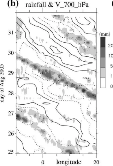
Figure 2.1 shows the Hovmoller (longitude versus time) plot of precipitation and the meridional component of the wind at 700 hPa averaged between 7N and 16N for the period 25-31 August 2005. 700 hPa is the altitude at which African easterly wave (AEW) forms as instability of the African easterly jet on its southern and northern side (Berry and Thorncroft, 2005). Interaction between MCS and AEW has been reported by many authors (e.g. Berry and Thorncroft (2005) and Mekonnen et al. (2006)), deep convective organisation seems to be favoured by the presence of AEW and diabatically generated potential vorticity anomalies has a role in sustaining AEW activity. As captured by time longitude diagrams of meridional wind at 700 hPa (figure 2.1), numerous African easterly wave developed and propagated in the period 25 August onward. The propagation of the rain band produced by the MCS studied here seems to be embedded within the trough of an African easterly wave.
Figure 2.2 shows the longitude-time diagram of surface rainfall from the satellite precipitation estimates EPSAT-SG (Chopin et al., 2004; Berg`es et al., 2010) and TRMM-3B42RT (Huffman et al., 2007). Both satellite estimates show a westward moving MCS propagating at a speed of 15◦/day. Structure and time evolution of
the simulated MCS are similarly described by TRMM and EPSAT products while the amount of precipitation is higher for TRMM.
Figure 2.1: Rainfall (shaded) and meridional wind at 700 hPa (interval of 2.5 ms−1
between isolines). (Adapted from Guichard et al. (2010))
Figure 2.2: Longitude-time diagrams of surface rainfall, averaged over [7N,16N]. Contour are 1,2,3,4,5,10,15 and 20. EPSAT-SG (left) and TRMM-3B42RT (right); the black thick lines delineate the area where the EPSAT-SG rainfall estimate is greater than 2 mm. (From Guichard et al. (2010))
2.2 Model intercomparison in the frame of AMMA 27
intercomparison (see table 2.1), all the mesoscale models have been initialized with ECMWF analyses. All the mesoscale models include parameterizations, which vary in complexity, of surface, radiative, turbulent, convective and cloud processes. The size of the simulated domain differs among models, the horizontal resolution varies between ten to a few tens of kilometers, therefore, all of them made use of a parameterization scheme to describe subgrid convection.
Table 2.1: Model used, horizontal grid resolution M odelname Horizontal Ref erence
resolution
BOLAM 12 km Malguzzi et al. (2006) COSMO 28 km Doms and Schattler (2002) MesoNH 10 km Lafore et al. (1997) PROMES 15 km Arribas et al. (2003)
WRF 12 km Skamarock et al. (2005)
MOUM 60 km - global Pope et al. (2000) ECMWF IFS 35 km - global Bechtold et al. (2008)
Figure 2.3 shows the longitude versus time plot for model precipitation, to be compared with figure 2.2. All the model simulate, as observed, a westward-moving pattern in this area, with relatively close speeds among models. However, it is not always the dominant pattern. Indeed, rainfall is predicted at night to the east of the rainfall line in most models. The rainfall line itself is less well defined in MesoNH, COSMO and ECMWF IFS. MesoNH and MOUM are also characterized by widespread daytime convection east of 5E. The BOLAM model overestimates precipitation with respect to satellite estimates but well reproduce the longitudinal extension of the MCS. Furthermore it underestimated the speed of propagation and generates an eastward shifted precipitation pattern.
task for mesoscale models. Despite the fact that all the mesoscale models have been initialised with the same ECMWF fields and have similar horizontal resolution, relevant differences are found with respect to satellite estimates and among model’s representation of precipitation.
2.2 Model intercomparison in the frame of AMMA 29
Chapter 3
How to improve the model
scores? A simple data
assimilation approach
In the previous chapter we showed that meteorological simulations of deep convective events and of the precipitation associated with them in West Africa is a difficult task to be addressed by mesoscale meteorological models. This because of the complex interaction between processes at different spatial and temporal scales and because of the scarcity and sparsity of atmospheric measurements in the region that lead to low reliable global analyses/forecasts used as boundary and initial conditions for mesoscale models.
In this chapter we describe the implementation of an assimilation scheme aimed at improving convective representation and precipitation. The scheme is based on the use of satellite observations of cloud top brightness temperature (CTBT) to correct the model humidity profiles. In fact the simulation of convection and precipitation is strongly dependent on an accurate description of water vapour profiles.
results are presented. Then the nudging procedure is tested against an intense precipitation event occurred between 9 and 12 August 2006 in West Africa. Precipitation and cloud top brightness temperature are used to evaluate the model capability in reproducing the deep convective event.
3.1
Observations used
During the monsoon season in West Africa the 80% of precipitation is expected to come from mesoscale convective systems that have a time-scale ranging from 1 day to few days. Thus for assimilation purposes observations used to improve convection needs to be at sufficiently high temporal resolution.
Global datasets of precipitation from rain gauges like GPCC (Rudolf and Schneider, 2004) are sparse and have low temporal resolution (1 month). Combined satellite and ground precipitation estimates of the Global Precipitation Climatology Project (GPCP 1DD) (Huffman et al., 2001) have the advantage of being continuous in space, but have a horizontal resolution of 1◦and a temporal resolution
of 1 day. Near-real-time satellite precipitation estimates from infrared and merged infrared and passive microwave instruments have a higher temporal (6 hours to 15 minutes) and spatial (0.7◦ to 0.1◦) resolution, but exhibit a low detection
rate for heavy precipitation in the tropics (Ebert et al., 2007). Moreover multi-satellite measurements need to be converted into precipitation estimates by means of parameterization and calibration that could introduce errors.
In the nudging scheme developed herein CTBT from 10.8 µm channel of SEVIRI radiometer on-board the Meteosat Second Generation Satellite (MSG) is used. It has been preferred to rainfall because its derivation from MSG radiance is a straightforward calculation and because it has higher temporal (15 minutes) and spatial (3 km at the sub-satellite point) resolutions with respect to rainfall estimates that also uses satellite radiance and has a time resolution of 3 hours and a spatial
3.1 Observations used 33
resolution of 0.25◦ (TRMM products).
A CTBT lower than 230 K is considered as a proxy for the occurrence of deep convection following Fu et al. (1990) where is shown that very little bright-cold clouds (organised convective systems) occurs at temperature warmer than 230K and very little dull-cold cloud (thin cirrus) occurs at temperature colder than 230K. A detailed description of the method used to derive CTBT from radiance is described in EUMETSAT (2008)
To evaluate the model, CTBT, TRMM 3B42 and GPCP 1DD precipitation estimates are used. The GPCP algorithm combines precipitation estimates from several sources, including infra red (IR) and passive microwave (PM) rain estimates, and rain gauge observations (Huffman et al. (2001) and references therein). The IR data came mainly from the different geostationary meteorological satellites but data from polar-orbiting satellites were also used to fill in the gaps at higher latitudes. The IR-based estimates used the Geostationary Operational Environmental Satellite (GOES) precipitation index (GPI). The microwave data come mainly from the Special Sensor Microwave Imager (SSM/I) onboard the defense meteorological satellite program. The PM estimates were used to adjust the GPI estimate. Then the multisatellite estimate was adjusted towards the large-scale gauge average for each grid box. The gauge-adjusted multisatellite estimates were then combined with gauge analysis using a weighted average, where the weights are the inverse error variances of the respective estimates. The current products include a monthly analysis at 2.5◦×2.5◦ grids, a 5-day (pentad) analysis at the
same spatial resolution, and a daily product at a special resolution of one degree.
The GPCP one-degree daily (1DD) product does not use PM rain estimates and gauge measurements directly (Huffman et al., 2001). SSM/I data were used within the framework of the threshold-matched precipitation index to delineate rain areas in the IR data. Gauge data were involved indirectly when the 1DD product was scaled so that monthly accumulations of 1DD matched the monthly
GPCP product. The monthly and pentad analyses extend from 1979 to current, while the daily product is available starting from October 1996. The daily products are made available 2 to 3 months after the end of each month.
Products from the TRMM multisatellite precipitation analysis algorithm include the ’TRMM and Other Satellites’ (3B42) described in Huffman et al. (2007). The 3B42 estimates are produced 3-hourly at a spatial resolution of 0.25◦. The
major inputs into the 3B42 algorithm are IR data from geostationary satellites, PM data from the TRMM microwave imager (TMI), SSM/I, Advanced Microwave Sounding Unit (AMSU) and Advanced Microwave Sounding Radiometer-Earth Observing System (AMSR-E). The 3B42 estimates are produced in four steps: (1) the PM estimates are calibrated and combined, (2) IR precipitation estimates are created using the PM estimates for calibration, (3) PM and IR estimates are combined, and (4) the data are rescaled to monthly totals whereby gauge observations are also used indirectly. This product is available for a few days after the end of each month.
3.2 The BOLAM model 35
3.2
The BOLAM model
BOLAM is a meteorological model based on primitive equations in the hydrostatic approximation. It solves the prognostic equations for wind components u and v, potential temperature, specific humidity and surface pressure. Variables are defined on hybrid coordinates and are distributed on a non-uniformly spaced Lorenz grid. The horizontal discretization employs geographical coordinates, with latitudinal rotation on an Arakawa C-grid. The model implements a weighted average flux scheme for three-dimensional advection. The lateral boundary conditions are imposed by means of a relaxation scheme that minimizes wave energy reflection. The microphysical scheme has five prognostic variables (cloud water, cloud ice, rain, snow and graupel), as derived from the one proposed by Schultz (1995). Deep convection is parameterized with the scheme of Kain-Fritsch (Kain and Fritsch, 1990; Kain, 2004). The boundary layer scheme is based on the mixing length assumption and the explicit prediction of turbulent kinetic energy (Zampieri et al., 2005), while the surface turbulent fluxes are computed according to the Monin-Obukhov similarity theory. The parameterization of the effects of vegetation and soil processes (Pressman, 1994) is based on the water and energy balance in a four-layer soil model, and includes the diagnostic computation of skin temperature and humidity, seasonally dependent vegetation effects, evapo-transpiration and interception of precipitation. The radiation is computed with a combined application of the scheme from Ritter and Geleyn (1992) and the operational one from the ECMWF (Morcrette et al., 1998). Further details of the model are provided in Malguzzi et al. (2000).
3.3
Description of the MCS event
The event used to perform the test of data assimilation is characterised by the development of two large mesoscale convective systems observed in the Sahelian
region from 9 to 12 August 2006. It has been chosen because is one of the strongest convective event of the 2006 monsoon season and because a validation of the nudging scheme for this case of intense precipitation was useful for the analysis of aircraft measurements presented in chapter 5.
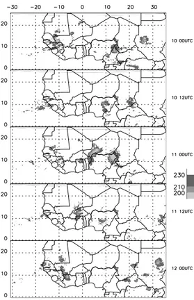
Figure 3.1: Meteosat cloud top temperature from 00 UTC 10 Aug. to 00 UTC 12 Aug. 2006, every 12 hours. Colour scale in K.
Figure 3.1 shows the CTBT derived from channel 10.8 of the SEVIRI instrument on-board the Meteosat Second Generation Satellite (MSG). The top panel refers to 00 UTC 10 August 2006 and the interval between two images is 12 hours. Two systems are clearly visible in the top panel: a westward system (WS) around 13E 10N and an eastward system (ES) around 26E 13N. The WS has a lifecycle longer than two days, with a decreasing phase at 12 UTC 11 August, followed by regeneration. Its approximate speed of propagation is 11 m/s and the minimum
3.3 Description of the MCS event 37
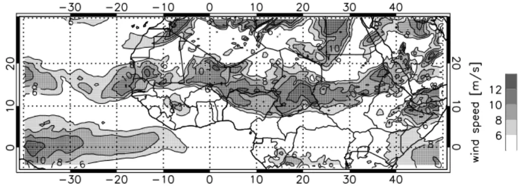
Figure 3.2: ECMWF analysis of wind speed at 700hPa on 00 UTC 10 Aug. 2006.
CTBT is 190K. The ES has a shorter lifecycle of 36 hours and dissolves over northern Nigeria around 12 UTC 11 August. Its propagation speed is similar to that of the WS system and its minimum brightness temperature is 185K.
The generation of these large systems is related to the intense monsoon flow, which is well established, providing favourable conditions for the generation of convection. The relationship of the observed MCS with the AEW activity is less clear. The wavelet decomposition presented in Janicot et al. (2008) shows that the AEW activity during the 2006 monsoon season was divided into three peak periods: mid-June, mid-July and from mid-August to mid-September. According to Janicot et al. (2008), the analysed event occurs in a period of low AEW activity. However, it is possible to identify the wave structure in the western part of the Sahelian region. Figure 3.2 shows the ECMWF (European Centre for Medium-range Weather Forecast) analysis of wind speed on 10 August at 00 UTC at 700hPa, considered as the altitude of maximum AEW intensity. A trough of an AEW is visible over South Mali. The ECMWF analysis 24 hours later (not shown) indicates that the wave moves westward toward Senegal. Nevertheless, it is difficult to relate the generation of the observed systems directly to this wave event.
3.4
Nudging procedure and simulation set-up
The nudging scheme is based on the approach proposed by Davolio and Buzzi (2004) (which is an evolution of the Falkovich et al., 2000 approach), focusing on the nudging of precipitation in extratropical regions. The scheme is modified here to deal with intense convective precipitation in the West African monsoon season: (1) the separation between convective and stratiform precipitations is not included and (2) the scheme assimilates the CTBT derived from the SEVIRI infrared channel centred at 10.8 micrometers, instead of precipitation. This has the advantage of a high spatial and temporal resolution and overcomes the uncertainty associated with precipitation estimates (Ebert et al., 2007).
The nudging procedure compares brightness temperature observed from satellite and evaluated by BOLAM and makes the appropriate modifications on the model specific humidity profile. Modifications are made when the temperature difference exceeds 2 K and when model or observed brightness temperatures are below 230 K, the latter condition to select only the grid points where precipitating deep convection occurs or is forecast by the model (Fu et al., 1990). The model-derived CTBT is estimated with the RTTOV-8 (Saunders et al., 2005) radiative transfer model from BOLAM water vapour, temperature and hydrometeors profiles.
The mixing ratio q(k), evaluated by BOLAM at each model level k and each grid point , is modified for the grid-point column selected for nudging according to the following equations:
q(k) = q(k)model+ ∆q(k)nudg (3.1) ∆q(k)nudg = −ν(k)τ−1[q(k)model−εqsat(k)] × ∆t (3.2)
where qsat is the saturation mixing ratio with respect to liquid water above
3.4 Nudging procedure and simulation set-up 39
a combination of saturation mixing ratio over liquid water and ice from Tetens’ formulas.
ν(k) is a weighting function that identifies the portion of the vertical profile modified by the nudging procedure. Parameter ν is set to 1 between the ground and 700 hPa, and then decreases to 0 at 500 hPa following a cubic law, remaining equal to 0 up to the top of the domain.
Parameter τ is the relaxation time that determines the intensity of nudging, it has been varied to test the sensitivity of BOLAM to the nudging scheme. The values used for the test are 2, 4 and 10 hours.
The sign and intensity of the modification applied to the moisture profile depend on the term in the square brackets in Equation (3.2). If BOLAM CTBT is greater than the satellite one (less intense convection), parameter ε in equation 3.2 is set to 1 and the humidity profile is increased toward its saturation value. In the opposite case, ε is set to 0.5 and the profile is decreased toward a sub-saturated condition. The subset of grid points where the nudging is applied and the value of parameter ε are determined by the comparison between model and satellite CTBT, performed every 20 minutes, while the satellite data are updated once per hour. The modification to the moisture profile is applied after the evaluation of the term in the square brackets of Equation (3.2), which is done for every integration timestep. This allows a smooth forcing of the model and the reduction of the forcing term, if the model profile approaches the target profile εqsat
.
A set of simulations was defined, using nudging with different assimilation periods and relaxation times, while a simulation without nudging was used as reference for the assessment of nudging impact. All simulations cover a period of three days from 00 UTC 09 August 2006 to 00 UTC 12 August 2006: better performances are obtained with a three day simulation starting when the two MCSs began to develop, in order to include their complete life cycle. Initial and lateral boundary conditions are interpolated from the ECMWF 6-hourly analyses
at 0.5◦×0.5◦ horizontal resolution and at 91 vertical levels.
The BOLAM model (described in section 3.2) is run with 38 vertical hybrid levels, from the ground to the top of the atmosphere (0.1 hPa), with denser levels near the ground. The horizontal domain chosen for the simulation has 300×220 grid points with a horizontal resolution of 12 km (0.108◦ in rotated coordinates). The
domain covers the region of the analyzed convective systems life cycle and ranges from 8W, 25E in longitude and from 2S to 23N in latitude. The large distance covered by Sahelian MCSs, due to their speed of propagation, requires the use of a large domain to describe their whole lifecycle, and, as a practical consequence, a reduced horizontal resolution. Thus convection cannot be explicitly risolved in the model and the use of a convective parameterization is needed.
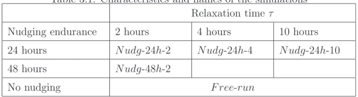
The values of the nudging window and the relaxation times are given in Table 3.1. Assimilation of CTBT through the nudging scheme starts after one day of free model integration (00 UTC of 10 August). According to sensitivity studies, a longer assimilation period does not improve the model performance nor the duration of improvements due to assimilation in the last day of simulation. The Nudg-24h-2 and Nudg-48h-2 simulations will be used to evaluate the impact of nudging duration on the rainfall and convective life cycle. The 24h-2, 24h-4 and Nudg-24h-10 experiments will be used to evaluate the sensitivity to the relaxation time τ defined in Equation 3.2
Table 3.1: Characteristics and names of the simulations Relaxation time τ
Nudging endurance 2 hours 4 hours 10 hours 24 hours N udg-24h-2 N udg-24h-4 N udg-24h-10
48 hours N udg-48h-2
3.4 Nudging procedure and simulation set-up 41
3.4.1
Sensitivity tests
In the present section we investigate the response of the BOLAM model to the modification of the weight assigned to the forcing term modulating the moisture profile. We focus on the sensitivity to the relaxation time τ , since it has a strong impact on the scores considering CTBT. The tests were run only on the 24 hour nudging simulations. The values tested for the τ parameter are 2, 4 and 10 hours. A further aim of the work was to assess the feasibility of producing accurate analyses based on radiance temperature nudging. Since τ determines the intensity of nudging, it is crucial to choose a smooth relaxation of the model towards the observations, for a long period of nudging. Fractional Skill Score (FSS, Robert and Lean 2008) was used to evaluate the performance of the model, in terms of CTBT (and rainfall in the following section). FSS scores belong to the verification methods based on fuzzy logic (Ebert, 2008), which relax the requirement for exact matches between forecasts and observations, using instead a spatial window or neighbourhood surrounding the forecast and observed points.
The percentage of grid points over the domain with CTBT under 220K is shown in the left panel of Figure 3.3 for the three analyzed simulations. This temperature threshold was chosen to evaluate the performance of the model in reproducing deep convective events, because 220K roughly corresponds to a cloud top above 12.5 Km height (Schmetz, 1997). In both panels the vertical lines indicate the start and the end of the assimilation period. In left panel it can be seen that the best matching between the MSG data is obtained with the simulation Nudg-24-2 for the first 62 hours of the run, after which an underestimation of the area covered by convection is visible. The right panel in Figure 3.3 shows the time evolution of the FSS score during the nudging period. It shows higher values for the maximum and a more rapid increase of the score for lower relaxation times. On the third simulation day, when the nudging scheme was inactive, the best performance of the model is still obtained with the experiment that has the lowest relaxation time, since the
simulation with τ =2 h shows the longest endurance of the improvement due to nudging. Such behaviour can be explained by the fact that a lower relaxation time implies a stronger forcing of the model toward the target given by the observations. Nevertheless, it must be stressed that the nudging directly modifies the water vapour content only in the lower troposphere, and a substantial agreement with a derived variable like infrared CTBT should be considered as a validation of the nudging approach. Thus, in the analysis below, we use the value of τ =2 h for both the 24 hour and the 48 hour nudging experiments.
Figure 3.3: Evolution in time of the percentage of grid points characterized by a CTBT exceeding 220 K [left panel]. FSS score versus time for CTBT, temperature threshold is 220 K and spatial window is 60 Km [right panel].
3.5 Comparison of simulated MCS lifecycle with observations 43
3.5
Comparison of simulated MCS lifecycle with
observations
3.5.1
Cloud top brightness temperature
The first objective was to evaluate the spatial and temporal distribution of the convective systems reproduced by the Free-run and the nudged simulations. The purpose was to assess the impact of the nudging procedure on the convective system representation and to evaluate the duration of the improvements derived from nudging. The evaluation here was carried out using observed and model-derived CTBT, because it is a good proxy for the intensity of convection. The simulations analyzed were Nudg-24h-2, Nudg-48h-2 and the Free-run; it has been chosen to use τ=2 h because it gives the best scores for CTBT, compared to the other relaxation times tested, as discussed in Section 3.4.1.
The CTBT at 18 UTC 10 August 2006 for the three simulations and MSG observations are shown in Figure 3.4. The Westward mesocale convective system (WS) and Eastward one (ES) are visible in the observations (top left panel) over northern Nigeria (WS) and southern Chad (ES), respectively. The ES appears to be more intense in terms of brightness temperature and area coverage. Sparse intense convective activity is also observed in northwestern Niger, Eastern Mali and Burkina Faso. The brightness temperature from the Free-run (Fig. 3.4, top right panel) is severely underestimated: convective systems in the latitude belt ranging from 5N and 15N appear to be smaller, less intense and less organised than observed. The Free-run simulation reproduces two distinct areas of intense convection: a western one over Nigeria, which is southerly displaced and less intense compared to satellite observations; an eastern one over southern Chad, now reproduced as sparse and intense convective activity and displaced eastward.
Nudg-24h-2 and Nudg-48h-2 (Fig. 3.4, bottom panel) are identical, since the nudging process is still active at the analyzed time for both simulations.
The nudging provides a substantial improvement on the MCS distribution and propagation. Both the position and the overall structure of ES and WS agree well with observations, even if the simulated MCSs are more scattered. The BOLAM brightness temperatures now lies within the same range as the MSG ones, even if the area covered by the MCS seems to be underestimated. The nudging reduces the cloud coverage and the intensity of the unrealistic convective activity at the boundaries between Nigeria and Cameroon, and allows the generation of small MCSs in the northern part of the domain.
Figure 3.4: Cloud top temperature at 18 UTC 10 Aug. 2006. MSG (top left), Free-run (top right), nudged simulations (bottom left). Colour scale is in K.
Figure 3.5 shows the observed and simulated brightness temperature at 18 UTC 11 August. It should be stressed that the simulation Nudg-24h-2 had 18 hours of run without assimilation after the 24 hour nudging, while Nudg-48h-2 was still
3.5 Comparison of simulated MCS lifecycle with observations 45
forced with MSG data. The observations show that the WS system is located in the 9N-18N belt around 5W longitude. The WS is weakening (as displayed by the lower BT values), while the ES is nearly dissolved, except three smaller cloud systems located above Benin and western Nigeria. Apart from the WS system and a small one in middle of Chad, convective activity north of 10N is absent. The Free-run simulation (Fig. 3.5, top right panel) shows a much more intense convective activity than the satellite. It reproduces organized convective activity in three areas, plus some small and intense convective systems.
The bottom left panel of Figure 3.5 (Nudg-24h-2) shows the evolution of the WS and the ES described above. The former is located between 10N and 17N and between 5W and 0, while the latter is the convective complex with its highest convective activity centred at 13N 5E. Both systems have moved slower than the observed ones and are slightly displaced northward. As regards the system evolving from the ES, it is still in an active (and intensifying) phase, rather than in a decreasing phase, as observed in the satellite data. The Nudg-48h-2 simulation (Fig. 3.5, bottom right panel) is in better agreement with the observations, as expected, since the nudging process is active throughout the entire run. Nevertheless, the 48 hour nudged simulation does not completely dissipate the WS, as in the case of Nudg-24h-2 simulation.
Figure 3.6 shows the 12.5 percentile of grid points where the CTBT exceeds the thresholds of 210K, 220K, 230K and 240K, for each fixed longitude in the domain, as a function of time. The cloud fraction colder than the threshold from MSG observations (Fig. 3.6, upper left panel) shows the time and longitude evolution of the two large MCSs described in section 2. Both systems are characterized by a marked diurnal cycle with development of convection after 12 UTC, a maximum around 18 UTC and a rapid decrease from 6 UTC to 12 UTC. This is in agreement with the convection cycle evaluated from the MSG climatology over Africa presented in Laing et al. (2008).
3.5 Comparison of simulated MCS lifecycle with observations 47
The Free-run simulation (Fig. 3.6, top right panel) forms three convective systems, which propagate westward with a reduced speed compared with observations. A realistic diurnal cycle is reproduced with generation of convection at 12 UTC on each simulation day and a maximum around 18 UTC. From CTBT maps at 14 UTC (not shown), it is possible to observe that convection initiates on the lee side of the Darfur mountains, in agreement with the analyses of Laing et al. (2008) and Mekonnen et al. (2006).
The Nudg-24h-2 simulation (Fig. 3.6, bottom left panel) has a correct position and propagation speed of the MCSs during the assimilation period (00 UTC 10 August - 00 UTC 11 August). After the end of the nudging period the speed of the two systems decreases and their lifecycle is not correctly reproduced. In fact, the ES does not totally dissipate at 6 UTC 11 August, but grows again at 12 UTC 11 August, while the WS decreases after 12 UTC 11 August. In general, the convective systems reproduced during the portion of simulation without nudging are characterized, as in the Free-run, by a lower westward propagation speed, but display a diurnal lifecycle of the systems in agreement with observations. It is also possible to argue that nudging has a relevant impact throughout the run since the convection on the last day of simulation, despite the mentioned differences, seems to be more realistic than in the Free-run. Figure 3.6 confirms that the Nudg-48h-2 simulation is in good agreement with the observed lifecycle and propagation speed of the MCS, even if it can be observed that convection is still active after 6 UTC 10 August between 0E and 10E, as in the case of the Nudg-24h-2 simulation.
The left panel in Figure 3.7 shows the percentage of grid points with CTBT under 220K. For both panels the vertical lines indicate the start of the assimilation period for both the nudged simulations and the end for the Nudg-24h-2 simulation. MSG observations again show the diurnal cycle of the convective activity, which is also, at least on a qualitative basis, reproduced by all simulations. Compared to the Free-run, the amount of convection is much better reproduced when the
Figure 3.6: Hovmoller plots for the 12.5 percentile of grid points whose CTBT exceeds the temperature thresholds of 210K, 220K, 230K and 240K, for each fixed longitude in the domain. Solid lines in the left borders indicate the nudging period.
3.5 Comparison of simulated MCS lifecycle with observations 49
assimilation is applied. The Free-run underestimates the average convective activity during the first two days of the simulation and overestimates it during the last one, while the nudged simulations underestimate the convective activity for just the first 30 hours, and capture a secondary maximum at 4 UTC 10 August as well as the rapid increase after 12 UTC 10 August. It is also worth noticing that, during the third day of the run, the Nudg-24h-2 simulation still shows a better agreement with MSG observations than the Free-run does. The right panel in Figure 3.7 shows the time evolution of the FSS. A maximum threshold of 230 K to calculate the FSS is chosen to apply the score only to the model grid points where the nudging procedure was active. The FSS analysis also shows a quantitative improvement as a result of the nudging procedure. From the start of the nudging period FSS rapidly increases up to values close to 0.85, after which the FSS for Nudg-48h-2 remains higher than in the Free-run until the end of the simulation, while the FSS for Nudg-24h-2 drops to values close to those of the Free-run after 13 hours from the end of nudging. This also provides an estimate of the endurance of the improvement due to assimilation.
Figure 3.7: Evolution in time of the percentage of grid points characterized by a CTBT exceeding 220 K [left panel]. FSS score versus time for CTBT, temperature threshold is 220 K and spatial window is 60 Km [right panel].
3.5.2
Rainfall
The next step was to assess to what extent the nudging improved the spatial distribution and intensity of the precipitation field. The comparison was performed for the last 24 hours of simulations, i.e. 11 August 2006. The rainfall observations came from the daily accumulated precipitation at 1 degree of the GPCP project (Huffman et al., 2001) and from the Tropical Rainfall Measuring Mission (TRMM) (Kummerov et al., 2000) 3 hourly product at 0.25 degree of resolution. Nicholson et al. (2003 I and II) used a rain gauge database, different from the one used by GPCP and TRMM estimates, to validate both TRMM and GPCP rainfall products over West Africa on 1998. They used an horizontal resolution of 2.5 degrees and showed that GPCP relative error lies between -2% and 14% in August. They showed also that TRMM relative error is around 8% in August, considering 1 degree boxes.
Figure 3.8 shows the accumulated precipitation for GPCP, TRMM and the simulations. Both rainfall datasets show two main precipitation areas associated to the ES and WS convective systems: West of 5E and between 10E and 15E. The precipitation of the Free-run simulation is associated to the three systems described in Figure 3.5, which produce rainfall throughout the 10N-15N latitude band. The comparison between the Free-run and rainfall observations shows that the simulated precipitation is more spread, and that the geographical position of the intense precipitation (> 20 mm) does not agree with the observed one.
A clear improvement is obtained with nudging for both the Nudg-24h-2 and Nudg-48h-2 simulations. The first shows a remarkable coincidence with GPCP and TRMM for the areas of intense precipitation and a general reduction of the rainfall area. The agreement is further improved with the 48 hour nudging. This result is also confirmed by the FSS score, calculated for two precipitation thresholds, 10 and 20 mm, and a longitude-latitude window of 3◦×3◦ for GPCP product
and 0.75◦×0.75◦ for TRMM. FSS scores have been evaluated by remapping the
3.5 Comparison of simulated MCS lifecycle with observations 51
scores are reported in Table 3.2. As expected, the FSS score is in general higher for the Nudg-48h-2 simulation. The improvement is particularly relevant for the highest threshold (20 mm), where both Nudg-48h-2 and Nudg-24h-2 simulations give markedly higher scores compared to the Free-run. For the lower threshold (10 mm) the nudging still provides an improvement in terms of FSS score. Nevertheless, the difference compared to the Free-run simulation score is less pronounced, a finding that can be explained by observing that low precipitation is distributed over a larger area, located in the same latitudinal band for observations and all the simulations.
Table 3.2: FSS score for precipitation evaluated for three thresholds: 10 and 20 mm. The reference values are GPCP [top] and TRMM [bottom]. The neighbourhood window considered is 3◦×3◦ for GPCP and 0.75◦×0.75◦ for TRMM.
N udg-48h-2 Nudg-24h-2 F ree-run GPCP 10 mm 0.88 0.74 0.65 20 mm 0.64 0.64 0.43 TRMM 10 mm 0.77 0.58 0.43 20 mm 0.65 0.53 0.24
Table 3.3 reports the total rainfall amounts from GPCP, TRMM and the simulations. Total rainfall is the accumulated precipitation over the whole model domain for the 11 August. Three range (< 0.5; 0.5 ÷ 5; > 20 mm) are chosen to estimate the performance of the simulations for total, low and intense precipitation, respectively. area values are the percentage of grid points where precipitation lies within the above mentioned ranges. It is worth noticing that the GPCP and TRMM product does not only use MSG radiances, which are assimilated into the model, but also passive microwave satellite and gauge measurements, to evaluate
Figure 3.8: 24 hour cumulated rainfall on 11 Aug. 2006. GPCP (top left), TRMM (top right), Free-run simulation (centre left), 24h-2 (center right) and Nudg-48h-2 (bottom).Black solid contours on the three simulation panels reproduce the GPCP rainfall for the threshold of 10 and 30 mm.


![Figure 3.3: Evolution in time of the percentage of grid points characterized by a CTBT exceeding 220 K [left panel]](https://thumb-eu.123doks.com/thumbv2/123dokorg/4725390.45842/44.892.157.737.508.764/figure-evolution-percentage-points-characterized-ctbt-exceeding-panel.webp)

