Foodomics: LC×LC approach in modern food science

(1)

UNIVERSITÀ DEGLI STUDI DI MESSINA

Dipartimento di Scienze Chimiche, Biologiche, Farmaceutiche ed

Ambientali

Doctor of Philosophy in “Chemical Science”

_________________________________________________

Foodomics: LC×LC approach in modern food science

PhD Thesis

Tutor

Katia Arena

Ivana Lidia Bonaccorsi

Coordinator

Prof.ssa Paola Dugo

(2)

Index

Abstract 1

1.0 Introduction 2

1.1 Liquid chromatography from the origin to modern techniques 2

1.2 General trends and recent development in LC 9

1.2.1 UHPLC techniques 9

1.2.2 Multidimensional LC 11

1.3 Detection system 12

1.3.1 Solute or solvent property detectors 13

1.3.2 Selective or universal detectors 13

1.3.3 Mass or concentration sensitive detectors 14

1.3.4 MS ion sources 15

1.3.5 MS analyzers 16

References 21

2.0 Multidimensional liquid chromatography 23

2.1 Heart-cutting versus comprehensive 2D-LC 25

2.2 Theoretical aspects 29

2.2.1 Peak capacity 30

2.2.2 Orthogonality 32

2.2.3 Resolution 34

2.2.4 Sampling frequency 35

2.2.5 Dilution factors and limit to detection 37

2.3 Method development in LC´LC 38

2.3.1 Column selection 38

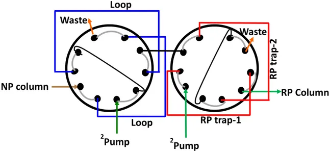
2.3.2 Modulation interfaces 39

2.3.3 Sampling 47

2.3.4 Mobile phase compatibility 47

2.3.5 Sample loop volumes 48

2.3.6 Elution modes in the second dimension 49

2.4 Detection 51

2.5 Data processing 52

2.6 Recent developments 53

References 58

(3)

3.1 Introduction to Foodomics 61 3.2 Foodomics applications: Challenges, advantages and drawbacks 62

3.3 Metabolomics 63

3.3.1 Metabolomics of Diet-Related Diseases 65

3.3.2 Analysis of Metabolome 66

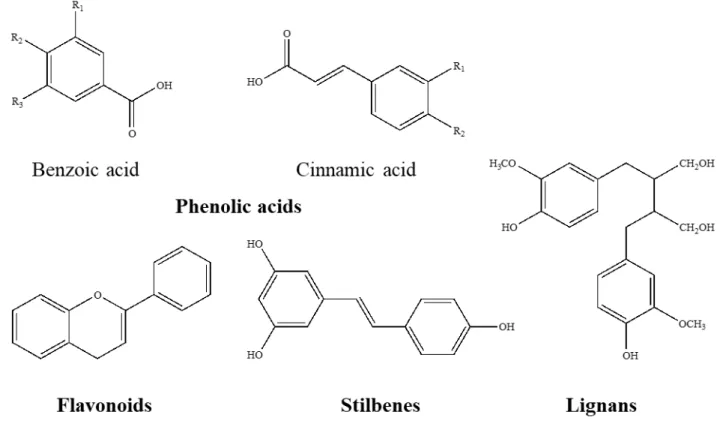
3.4 Polyphenols 67

3.4.1 Classes and structure of Polyphenols 69

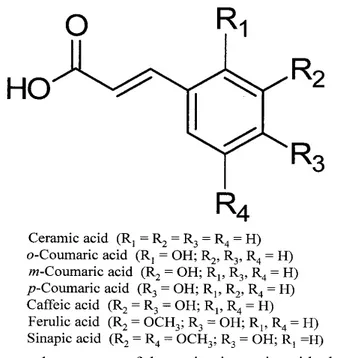
3.4.2 Phenolic acids 70

3.4.3 Flavonoids 72

3.4.4 Lignans 74

3.4.5 Stilbenes 74

References 76

4.0 Determination of the polyphenolic fraction of Pistacia vera L. kernel extracts by comprehensive two-dimensional liquid chromatography coupled to mass

spectrometry detection 78

4.2 Experimental 80

4.2.1 Reagents and Materials 80

4.2.2 Sample and sample preparation 81

4.3 Instrumentation and software 82

4.4 Analytical conditions 82

4.4.1 LC separation 82

4.4.2 LC×LC separations 82

4.5 Detection conditions 83

4.6 Data handing 83

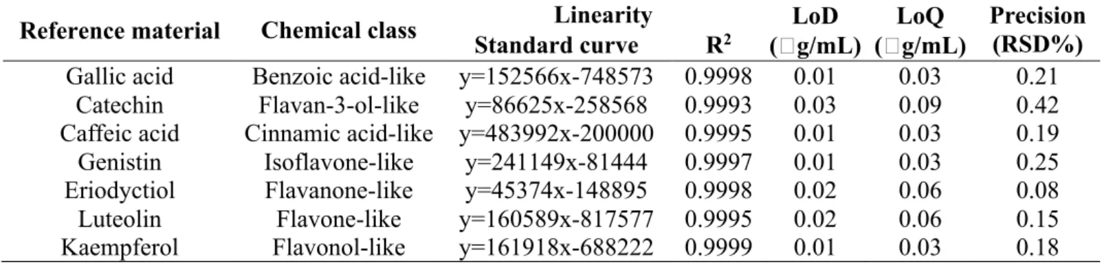
4.7 Construction of calibration curves 84

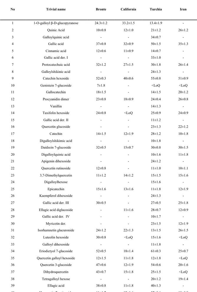
4.8 Results and discussion 85

4.8.1 RP-LC-PDA-ESI-MS analysis of the polyphenolic fraction of in Pistacia vera

extracts 85

4.8.2 Optimization of the RP-LC×RP-LC-PDA-ESI-MS analysis of the

polyphenolic fraction in Pistacia vera extracts 86

4.8.3 Semi-quantification of the polyphenolic fraction

of in Pistacia vera extracts by RP×RP-PDA-ESI-MS analysis 92

4.9 Conclusion 94

(4)

5.0 Quantitative analysis of aqueous phases of bio-oils resulting from pyrolysis of different biomasses by two-dimensional comprehensive liquid

chromatography 98

5.2 Materials and methods 101

5.2.1 Reagents and standards 101

5.2.2 Biomass samples 102

5.2.3 Bio-oils production 102

5.3 LC × LC instrumentation 103

5.3.1 LC × LC separation conditions 104

5.4 Validation of the quantitative method 105

5.5 Other calculations 106

5.5.1 Peak capacity 106

5.5.2 Orthogonality 107

5.6 Results and discussion 108

5.6.1 LC × LC method optimization 108

5.7 Development and validation of the quantitative method 113

5.8 Analysis of bio-oils 116

5.9 Conclusion 123

References 124

6.0 Comprehensive two-dimensional liquid chromatography-based

quali-quantitative screening of aqueous phases from pyrolysis bio-oils 126

6.1 Introduction 126

6.2.1 Chemicals and standards 129

6.3 Biomass samples 129

6.4 Pyrolysis process and aqueous phase samples 130

6.5 LC × LC analysis 131

6.5.1 Equipment 131

6.5.2 Chromatographic conditions 131

6.5.3 Calculations 132

6.5.4 Quantitative method 133

6.6.1 LC × LC analysis of bio-oil aqueous phases 134

6.6.2 Qualitative and quantitative chemical characterization 137

(5)

References 146 7.0 Application of compressed fluid–based extraction and purification

procedures to obtain astaxanthin-enriched extracts from Haematococcus pluvialis and characterization by comprehensive two-dimensional liquid

chromatography coupled to mass spectrometry 148

7.2.1 Samples and Reagents 152

7.3 Pressurized liquid extraction 152

7.4 Supercritical antisolvent fractionation 153

7.5 Experimental design 154

7.6 Total carotenoid determination 156

7.7 Chemical characterization of H. pluvialis extracts and SAF fractions by

liquid chromatography coupled to diode array detection 156 7.8 Chemical characterization of H. pluvialis extracts and SAF fractions by

comprehensive two-dimensional liquid chromatography 157

7.9.1 Extraction of carotenoids from H. pluvialis 158

7.9.2 Characterization of extracts using comprehensive two-dimensional coupled

to mass spectrometry detection 167

7.10 Conclusion 171

8.0 Determination of the Metabolite Content of Brassica juncea Cultivars Using Comprehensive Two-Dimensional Liquid Chromatography Coupled with a

Photodiode Array and Mass Spectrometry Detection 174

8.2.1 Chemical and Reagents 177

8.2.2 Sample and Sample Preparation 177

8.3 Instrumentation 178 8.4 Analytical Conditions 178 8.4.1 LC Separations 178 8.4.2 LC×LC Separations 179 8.4.3 Detection Conditions 179 8.4.4 Data Handling 180

(6)

8.4.5 Construction of Calibration Curves 180

8.5 Results and Discussion 180

8.5.1 Elucidation of Brassica juncea Cultivars Using RP-LC×RP-LC-PDA-MS 181 8.5.2 Semi-Quantitative Determination of the Flavonoid Content of Brassica juncea

Cultivars 185

8.6 Conclusion 189

9.0 Polyphenolic compounds with biological activity in guabiroba fruits

(Campomanesia xanthocarpa Berg.) by comprehensive two-dimensional liquid

chromatography 192

9.2 Materials and Methods 192

9.2.1 Sample 194

9.2.2 Chemicals 195

9.3 Extraction of polyphenolic compounds and experimental design 195

9.4 Determination of total phenolic content 197

9.5 Determination of polyphenolic compounds by LC×LC 197

9.5.1 Chromatographic columns 197

9.5.2 Instrumentation and software 197

9.5.3 Analytical conditions 198

9.5.4 Validation of the quantitative method 199

9.5.5 Peak capacity and orthogonality 200

9.6. Biological activity 201

9.6.1 α-amylase inhibitory activity 201

9.6.2 α-glucosidase inhibitory activity 202

9.6.3 Antioxidant analysis by survival assay 203

9.7. Statistical analysis 203

9.8. Results and discussion 204

9.8.1 Effects of the solvent system on phenolic compounds extraction 204

9.8.2 LC×LC method optimization 206

9.8.3 Development and validation of the quantitative method 209 9.8.4 Profiling of polyphenolic compounds in guabiroba fruits 212

9.8.5 Antidiabetic and antioxidant properties 216

9.9. Conclusion 219

(7)

10.0 Evaluation of matrix effect in one-dimensional and comprehensive two-dimensional liquid chromatography for the determination of the phenolic

fraction in extra virgin olive oils 223

10.2.1 Chemicals and reagents 225

10.2.2 Samples and sample preparation 226

10.2.3 Instrumentation and software 226

10.3 Analytical conditions 227 10.3.1 LC separations 227 10.3.2 LC × LC separations 228 10.3.3 Detection conditions 228 10.3.4 Data handling 229 10.3.5 Method validation 232

10.4.1 RP-LC and RP-LC × RP-LC method validation 233

10.4.2 Evaluation of MEs of the RP-LC×RP-LC method for determination of the

phenolic compounds of extra virgin olive oils 236

10.5 Conclusions 238

(8)

Abstract

The object of the research work investigated in this Ph.D. thesis was the development and implementation of advanced analytical techniques based on comprehensive two-dimensional liquid chromatography coupled to MS, in order to obtain a complete identification and characterization of bioactive molecules in complex natural products. Comprehensive two-dimensional LC (LC×LC), involving the coupling of two or more orthogonal or quasi-orthogonal separation systems, is an interesting alternative to classical 1D approach, being in many cases also selective and sensitive enough to detect minor components. The advantages of this technique compare to mono dimensional approach are: increased resolving power, enhanced identification potential, especially when coupled to mass spectrometry, reduction of ion enhancement or suppression phenomena during the ionization process in the source of MS. In addition, modern food analysis is direct to the characterization of as many components as possible in food and food-related materials. The use of “Foodomics” approach requires the employ of these advanced analytical techniques, able to offer capability to separate a high number of constituents, such as LC×LC separations. For this reason, most of the research have been focused on the characterization of polyphenols compounds in food samples and natural products.

(9)

1.0 Introduction

1.1 Liquid chromatography from the origin to modern techniques

The term “chromatography” according to the International Union of Pure and Applied Chemistry (IUPAC) refers to a physical method of separation, in which, compounds of the samples are selectively distributed in two immiscible phases [1]. The history of modern chromatography can be located to the beginning of the 20th_{century, when the}

Russian botanist Michail Tswett (1872–1919) using a packed column with a calcium carbonate as stationary phase, was able to separate coloured pigments from plant extracts [2]. In his experiments, Tswett put the sample at the head of the column that were carried out through the stationary phase using a flow of petroleum ether used as mobile phase. As the sample moved through the column, the extracts were separated into individual coloured bands. Once the pigments were well separated, the calcium carbonate was eluted from the column and the pigments recovered by extraction. Tswett called the technique “chromatography”, combining the Greek words “chroma” (colour) and “grafos” (writing). There was little interest in Tswett’s technique until late 60’s, when thanks to the development in columns, detectors and the works of Martin and Synge, who developed the liquid-liquid partition chromatography for the separation of acetyl derivatives of natural amino-acids, and defined a chromatographic theory by adding the theory of distillation in packed columns [3]. The column could be divided into a series of "theoretical tables", each one showing a partition balance between various phases (stationary phase and gas phase during distillation, stationary phase and liquid phase in chromatographic processes). The efficiency is related to the theoretical plates, so correlated to the length of the column, or otherwise, reversely proportional to the “equivalent height of the theoretical plate (HETP o H). This latter dependes to variables that influence the diffusion of solutes in the two phases, like the diameter of the particle of the column, so that a larger porosity size results in a more

(10)

relevant diffusibility of the compounds in the stationary phase, thus enhancing the H value. The new parameter to be taken into account in chromatography is the flow rate of the mobile phase, in particular the diffusion described above can be minimized if a high flow rate is applied. In this respect, the capability to use a very high flow rate without any pressure restrictions and maximize the chromatographic performance was the main reason for the faster development of gas chromatography (GC) compared to LC. In 1956 was introducted, by Van Deemeter et al., the relative equation for GC process [4].

! = # +%

&+ '( (1)

According to this formula, H is the sum of the three terms:

1) A refers to the influence of multi-path dispersion across the column, due to potential packing differences or particles with various dimensions so multiple diffusion channels are formed; this parameter is also called Eddy diffusion and could be calculated as A=2λdp, where λ refers to the quality of the packing and

dp is the diameter of the particle.

2) B is the longitudinal diffusion, which follows the solute gradient of concentration, resulting in the Gaussian shape of each chromatographic peak. It can be represented as B=2γDM/u, where γ is, as λ, a variable connected to

potential differences in the stationary phase, DM is the diffusivity of the solute

in the mobile phase and u is the linear velocity of the mobile phase. To reduce the B factor, DM should be kept to a minimum and a high flow rate should be

used.

3) C is the resistance to mass transfer, considering both mobile (Cm) and stationary (Cs) phase transfer, then C = Cm+Cs, where Cm=f1K'dp2u/DM and

Cs=f2K'df2u/Ds. The parameters f1 and f2 are values related with the shape of the

(11)

retention, dp and df are respectively the particle diameter and the total packing, DM and

Ds are the diffusivity of the solute in the mobile and stationary phase, respectively, and

u is the flow rate of the mobile phase. This term was not considered before by Martin and Synge, who expressed only a direct proportionality between chromatographic efficiency and flow rate [5].

Due to the presence of two different contributions, it has been possible to establish that there an optimal flow is obtained when both terms B and C were minimized. It corresponded to the minimum of the traced curve H against the linear velocity u (Figure 1).

Figure 1. Typical Van Deemter plot

According to Van Deemter's equation it became obvious that the decrease of both particle diameter (dp) and stationary phase thickness (df) should cause a significant reduction of H, since both terms A and C are linked to these parameters. This was the work of Golay, who in 1958 wrote an article on open tubular columns equally coated with a thin layer of stationary phase, thereby removing the term A and making C

(12)

smaller due to the thinness of the stationary phase [6]. The direct result was an exponential increase in GC applications and open capillary tubular columns are re the most popular used nowdays. GC theory was promptly applied to LC, resulting in the development of high performance column packings for LC, substituting traditional 30-200 µm porous material with particles of less than 10 µm. The origin of modern LC is usually attributed to Horvath, who packed for the first time in 1965, a 1mm ID column with µ-porous particelles [7]. Based on column length, ID and particle dimensions, the mobile phase has been flushe into the column at different flow rates in the µL-mL/min range with relatively high back pressures. Therefore, high performance liquid chromatography or high pressure liquid chromatography (HPLC) has been the name of modern LC techniques, aiming to increase the separation of constituents and the repeatability of the method, thus enabling qualitative/quantitative analysis. The main columns used in LC have ID 2-2.1 mm or 4-4.6 mm and a length of 10-25 cm. Columns with smaller ID allow very low sample detection quantification but leading to a low sampling capacity. Bigger columns are generally utilized for preparatory LC. Table 1.1 shows the classification of analytical LC columns according to their ID [8].

The first stationary phases employed in LC by Tswett in 1903 were very polar chemicals such as cellulose, silica. In 1950 Martin and Howard discovered that very apolar components such as long chain fatty acids were not properly separated on a polar substrate, whatever the composition of the mobile phase used [9]. Subsequently, they combined a stationary phase in cellulose acetate and water in combination with a very apolar solvent such as octane to ensure good separation quality (high chromatographic resolution). New chromatography separation, in which the stationary phase was less polar than the mobile phase, was called reversed phase (RP) LC to differentiate it from conventional normal phase (NP) LC.

(13)

Table 1.1 Classification of LC columns according to their ID

Column designation Typical I.D. (mm)

Preparative LC Higher than 20

Semi- Preparative LC 6-20 Conventional LC 3-5 Narrow-bore LC 2 Micro LC 0.5-1 Capillary LC 0.1-0.5 Nano LC 0.01-0.1 Open tubular LC 0.005-0.05

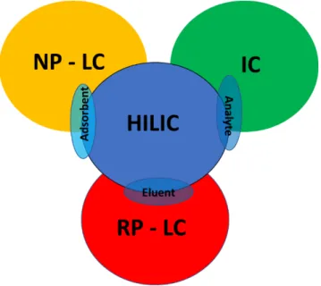
In normal phase liquid chromatography (NP-LC), the stationary phase is more polar than the mobile phase. Retention is higher as the polarity of the mobile phase decreases, so polar analytes are retained more strongly than non-polar analytes. Opposite situation occurs in reverse phase liquid chromatography (RP-LC). NP-LC has been extensively utilized to separate different compounds, from non-polar to highly polar compounds. Even though RP-LC systems were earlier widely employed by scientists, NP-LC methods are still in a phase of turnaround. Hydrophilic interaction liquid chromatography (HILIC) is another mode of high performance liquid chromatography (HPLC) for the polar compounds separation. Due to various reasons, HILIC has been described as a variant of normal phase liquid chromatography, but the separation mechanism used in HILIC is more complex than that of NP-LC. The number of publications on HILIC has increased substantially since 2003 as highlighted in the well-constructed review of Hemström and Irgum [10].

(14)

Such as NP-LC, HILIC uses traditional stationary polar phases such as silica, amine or cyan [8-12], but the mobile phase adopted is quite similar to those used in RP-LC mode [10-12]. HILIC also enables the analysis of charged substances, as in ion chromatography (IC). Figure 2 shows how HILIC is complementary to other areas of chromatography and extends the range of separation options.

Figure 2. HILIC combines the characteristics of the three major methods in liquid chromatography

HILIC offers several specific benefits over traditional NP-LC and RP-LC. For example, it is suitable for the analysis of mixtures in complex systems that always elute close to void in reserved phase chromatography. Polar samples always exhibit good water phase solubility in the mobile aqueous phase used in HILIC, which bypasses the problems of poor solubility often found in NP-LC. Expensive ion pair reagents are not needed in HILIC and can be conveniently combined with mass spectrometry (MS), especially in electrospray ionization (ESI) mode. Unlike RP-LC, HILIC gradient elution starts with a low-polarity organic solvent and elutes polar analytes by increasing the aqueous polar content [13]. A recommendable mobile phase would contain high

(15)

organic concentration for enhanced sensitivity and would also exhibit good column retention for polar ionic compounds. Hydrophilic interaction liquid chromatography has proven to be the separation mode of choice for uncharged highly hydrophilic and amphiphilic compounds that are too polar to be well preserved in RP-LC but have insufficient charge to allow effective electrostatic retention in ion exchange chromatography. HILIC separation is currently gaining a lot of popularity as it resolves many separation problems that were previously hard to solve, such as the separation of small organic acids, basic drugs and many other neutral and charged substances. It has been successfully applied to the analysis of carbohydrates [14,15], peptides [16-18] and polar drugs [11,19], etc.

Several articles have discussed the mechanism and theoretical description of analyte retention in HPLC. Basically, there are three different ways to model the separation process. The first is the partitioning of the analyte between the mobile and stationary phase [20, 21]; the second is the adsorption of the analyte on the adsorbent surface [22, 23]; the third takes the selective adsorption of the organic mobile phase modifier on the adsorbent surface, and then by the partitioning of this analyte in the adsorbent layer [24]. The retention phenomenon in HPLC depends at the same time on several types of intermolecular interactions among solute and stationary phase, solute and mobile phase, and stationary and mobile phases. The current theory suggests that HILIC retention is due to partitioning. This phenomenon still lacks an in-depth theoretical explanation. In this method, the separation mechanism is dependent on the differential distribution of the solute molecules of the injected analyte between the mobile phase rich in acetonitrile and a layer enriched with water adsorbed on the stationary hydrophilic phase [25,26]. Therefore, the more hydrophilic the analyte, the more the distribution equilibrium is shifted towards the immobilized water layer on the stationary phase, the more the analyte is retained. This means that a separation based on the polarity of the compounds and the degree of solvation takes place.

(16)

1.2 General trends and recent development in LC

1.2.1 UHPLC techniques

Over the last years, chromatographers continued to focus their attention on reducing column particle diameters in order to improve chromatographic efficiency with reasonable flow rates, resulting in a considerable reduction in analysis time. As shown by Giddings in 1991 there is a linear correlation between the pressure drop (ΔP) and the linear velocity (u) in the column [27] (equation 1.2).

∆* =

,h-._/

!

"

(2)

where φ, h, L and d are the flow resistance, mobile phase viscosity, column length and diameter of the particles, respectively. It has been proved that choosing a 25cm lengthy column packed with 5 µm particles, an inlet pressure less than 25bar is needed to perform the analysis, while reducing the particle diameter at 1 µm require an inlet pressure of 2000 bar [28,29]. Therefore, a significant upgrade of the instrumentation was essential: the pumps, the injection system and all connections had to be able to work at very high pressures (thousands of bar), instead detectors capable of acquiring a high acquisition speed had to be used. The name of the new instrumentation and new methods was ultra-high pressure (or ultra-high performance) LC (UPLC or UHPLC), a term coined by Jorgensen in 1997 [30] and used today to refer to a very fast separation with high efficiency and resolution. The heart of the UHPLC technique lies in columns with particles smaller than 2 µm. Observing Van Deemter's diagram for this type of columns (Figure 3), it is possible to see the flattening of the curve in the region of linear velocity of mobile phase greater than optimal, which means that these columns can run at high flow rates without any loss of efficiency.

(17)

Figure 3. Van Deemter Plot at different dp

Figure 3 shows similar performance for the other packing of columns, i.e. monolithic and with fused-core. The first was introduced roughly in the same years of sub-2µm particles and consists of a single piece of porous material such as organic polymers or silica, having a very limited flow resistance compared to a particle-packed column. Normally the diameter of the porous rod is about 1.5-2 µm (macroporosity) with porosity of 10-12 nm (mesoporosity), which minimizes the diffusion path and mass transfer effect. However, mesopores make these columns not very efficient for small molecules, on the contrary, they are largely still employed for the analysis of macromolecules, like in proteomics analysis [31]. The biggest problem with monolithic technology is the limited length of the column: a straight monolithic column longer than 15 cm cannot be prepared smoothly, thus limiting the number of theoretical plates per column. [32,33]. Fused core particles appeared on the market in 2006 and are also called as partially porous or core-shell particles to discern the difference with totally porous technology and the presence of a solid core in which analytes cannot penetrate. The biggest advantage of the fused core columns compared to columns of less than 2 μm is the lower backpressure so that these phases can be operated on a conventional LC instrument [34].

(18)

1.2.2 Multidimensional LC

Within the overview of LC trends, recent improvements in multidimensional techniques should be reported. Actually, multidimensional LC (MDLC) has a history almost as long as chromatography. The term is used to refer to the coupling of more than one column to separate sample compounds, where each mechanism of separation in each column being an independent separative dimension. The necessity to develop MDLC methods was born from the extreme complexity of several real samples, since the one-dimensional system was not able to fully resolve all the components of the sample mixture. For example, in the presence of biological or pharmaceutical samples, the separation of enantiomers is very important; therefore a first dimension (1D) is used to separate the diastereoisomers, and a properly time-controlled transfer of each peak into a second dimension enantioselective (2D) is used to resolve the enantiomers. Basically, there are two types of multidimensional LC approaches: the heart cutting (LC-LC) and comprehensive (LC×LC). The first one, allows 2_{D separation for selected}

fractions of the sample only, while the second allows the two-dimensional (2D) separation of the whole matrix with a significant increase in resolving power, which is usually given by the total peak capacity (nc), which is the number of analytes that can

be theoretically separated.

The two approaches may be carried out both in off-line and on-line modes. In the former case, the fractions eluted from the first column are collected manually or from a fraction collector, concentrated if necessary, and re-injected in a second column. These solutions are certainly time-consuming, labor-intensive and difficult to automate. In addition, off-line sample treatments might be prone to contamination resulting not useful if quantitative trace analysis is required. This technique is most commonly employed when only specific parts of the first separation require secondary separation. In an on-line MDLC system instead, the two columns are connected through a special interface, usually a switching valve, which enables the transfer of the

(19)

fractions from the first column effluent to the second column. This approach should fulfill some specific criteria, like as compatibility of the 1_{D mobile phase and the}2_D

stationary phase, the miscibility of the solvent used in the two dimensions, and the elution time in the 2_{D must be very fast, before the successive transfer. Stop flow}

approach, where the 1_{D flow is temporarily interrupted during the elution in}2_D,

allowed to go over this issue. Otherwise, a very high flow rate or a short column can be used to accelerate the separation in 2D, affecting the chromatographic efficiency according to Van Deemter's equation. However, the development of UHPLC and improvements in stationary column phase technology have made possible to perform very fast analyses without losing efficiency. Nonetheless, the need for a specific interface and software, the skill level of the operator and also the cost implications make online techniques less easy to use than the off-line approach which can be easily realized because both analytical dimensions can be optimized as two independent methods.

1.3 Detection systems

Detector choice is usually key for the achievement of a particular HPLC method. A certain variety are in daily use, including UV, fluorescence, electrochemistry, conductivity and refractive index detectors, each with their own particular advantages and drawbacks. Detectors may be classified:

• solute or solvent-property detectors • selective or universal detectors

• mass or concentration sensitive detectors •

(20)

1.3.1 Solute or solvent property detectors

This category covers whether the detector detects in solute property (analyte), e.g. for the UV detector, or a variation of some solvent properties (mobile phase) caused by the presence of an analyte, e.g. for the refractive index detector.

1.3.2 Selective or universal detectors

This category takes into consideration whether the detector responds to a specific analyte property of the analyte of interest or whether it will respond to a high number of analytes, regardless of their structural properties. According to the classification, it can be assumed that solute detectors are also typically selective while solvent detectors are general detectors.

UV absorption is the most used HPLC detection technique is probably UV absorption and has capacity both as a specific detector and as a general detector, according on the way it is utilized. If the wavelength of maximum absorption of the analyte (λmax) is given, it can be controlled, and the detector can be considered selective for these analytes. As UV absorptions are, however, typically broad, this form of detection is often not selective. If a diode instrument is used, it is possible to monitor more than one wavelength and measure the absorbance ratio. Agreement of the ratio measured by the "unknown" with that measured in a reference sample gives better confidence that the analyte of interest is being measured, although it does not yet provide absolute certainty.

A broadly used general detector is the refractive index detector that measures variations in the refractive index of the mobile phase as an analyte elutes from the column. If gradient elution is selected, the refractive index of the mobile phase changes as its composition changes, giving a constant baseline of the detector. The measurement of both position and intensity of a low intensity the analytical signal on a variable baseline

(21)

is less exact and less accurate than the same measurement on a constant baseline with zero baseline signal. It is usually recognized that general detectors are not as sensitive as specific detectors, showing a lower dynamic range and do not provide the best results when gradient elution is utilized.

1.3.3 Mass or concentration sensitive detectors

The last classification concerns how intense the detector response is proportional to the solute concentration or to the absolute amount of solute that reaches it. This class of detector is really important for quantitative goals. If the flow rate of the mobile phase is increased, the concentration of the analyte reaching the detector remains the same, but the amount of analyte increases. In these conditions, the intensity of the signal from this kind of detector will stay constant, even though the peak width will decrease, i.e. the the response area will decrease too. A variation in the flow rate will decrease the width of the response of a mass sensitive detector, unlike a concentration sensitive detector, the signal intensity will increase as the absolute quantity of analyte reaches the detector. As the overall response increases, this can be used to improve the quality of the signal obtained. In many experimental conditions, mass spectrometer works as a mass sensitive detector, and in others, like for example when LC-MS is used in electrospray ionization, it can be considered like a concentration sensitive detector. A benefit of the mass spectrometer as a detector is that it can provide differentiation of compounds with very similar retention characteristics or may enable the identification and/or quantitative determination of compounds that are only partially eluted chromatographically, or even those totally co-eluted. In general, an MS instrument consists of three basic components, namely the ion source, to generate ions from the sample, the mass analyzer, to separate them according to the mass-to-charge ratio (m/z), and the detector, to measure emerging ions.

(22)

1.3.4 MS ion sources

According with the ionization process that take place into the ion source, mainly divided in hard and soft ionization, the level of information obtained is different. Hard ionization process provides enough energy to the molecules that involves bonds break, releasing fragment ions having a mass-to-charge ratios lower than the molecular ion, driven the structural elucidation. On the contrary, soft ionization leads to a less fragmentation, therefore the resulting mass spectrum usually includes the molecular ion peak (in GC-MS) or the deprotonated molecular ion (LC-MS), given the molecular weight details. Immediately after its invention, it became obvious that this technique was well adapted for volatile and thermally stable compounds, but it precluded the study of large molecules. In addition, due to poor compatibility of the liquid phase with the vacuum region of an MS, hyphenation with gas chromatography was simpler than hyphenation with LC, which needed to elimination of the mobile phase prior the analyte enters in the mass spectrometer, thus compromising analytical performance. The turning point arrived with the discover of different ionization techniques, like as, the atmospheric pressure ionization (API) and in particular the electrospray ionization (ESI) and atmospheric pressure chemical ionization (APCI). Thanks to these new techniques, the elimination of the quantity of the solvent was much easier [35,36]. Nowadays, ESI and matrix assisted laser desorption ionization (MALDI) are the techniques of choice for the analysis of macromolecules. In the first case, the ionization arrives after the passage of the analytes into a needle keep at high voltage (kV) placed at the entrance to the MS. ESI is the best technique for very polar compounds, ranging from 100 to 150000 Da. On the contrary, MALDI produces only singly charged ions, and it is suitable for protein and carbohydrate characterization [37]. Finally, APCI is preferred to ESI for the medium polarity compounds comprised for 100 to 2000 Da. While ESI is liquid phase ionization, APCI is in gas phase conditions, after a nebulization promoted by nitrogen stream and the subsequent LC effluent vaporization at 350-550 °C.

(23)

1.3.5 MS analyzers

The analyzer can be considered the heart of MS, since characteristics such as analysis speed, mass range, resolution, mass accuracy, dynamic range and sensitivity depend on it. The most widely used mass analyzers, due their low cost, are the quadrupole (Q), ion-trap (IT) and time of flight (ToF), as well as a mix of hybrid instruments such as Q-ToF, IT-ToF and QqQ (triple quadrupole). In general, the ToF analyzer is distinguished by a very high resolution, mass accuracy, analysis speed and very wide mass range. On the contrary, quadrupole and ion trap are limited to a specific m/z range that arrive to detector according to the electric field applied [38]. In the Figure 4 a schematic representation of quadrupole and ion trap detector is showed. In detail, quadrupole is made up of 4 metal bars to which a combination of current and radiofrequency is applied in order to send only specific ions; in fact, in ion trap the radiofrequency (RF) is released by a ring electrode, while a direct or alternate current (DC or AC) can be applied to the terminal electrodes, so that at the beginning the ions are present together inside the trap and are ejected by applying the RF field in a similar way to the quadrupole analyzer.

Figure 4. Schematic representation of quadrupole (on the left) and ion trap (on the right) analyzers.

Generally, MS systems can work in full scan mode (total ion current chromatogram, TIC), in tandem MS experiments or in selected ion monitoring mode (SIM) where only

(24)

ions with a given m/z value reach the detector by setting a specific RF on the quadrupole. SIM mode is used for the development of selective and sensitive quantitative method, due to the reduction of the baseline noise, i.e. the gain in the signal-to-noise ratio (S/N). In addition, the integration of the SIM spikes excludes any problem from totally or partially coeluted substances, as is the case with a PDA detector [39].

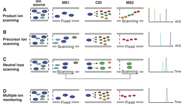
Nevertheless, the quantification, or even detection of a target trace component, in SIM mode can be tricky with high background ions of the same m/z values; in these cases, higher selectivity is achieved using MS/MS techniques. At this time, triple quadrupole (QqQ) instruments are the detector of choice for targeted analysis with high selectivity and sensitivity [40]. A schematic representation of this analyzer is shown in Figure 5.

Figure 5. Schematic representation of triple quadrupole

While Q1 and Q3 work as true quadrupoles by filtering ions according to the combination of RF and DC, q2 operates like an ion trap where only one RF is applied to capture the ion. If both Q1 and Q3 operate both in SIM mode, by choosing a precursor or "parent" ion and a produced or "daughter" ion respectively, maximum selectivity and sensitivity is achieved in the so-called selected reaction monitoring (SRM) or multiple reaction monitoring (MRM) mode. Normally, the fragmentation

(25)

marked by the highest S/N is chosen as a quantifying transition for quantitative analysis, while a second (or even more) fragmentation is selected as a qualifying transition, necessary to evaluate with a high level of certainty the identification of the components. Furthermore, the ratio between the intensity of the two transitions is typical of the given component and must remain stable along the linearity range [41]. The very low detection limit reduces sample consumption and also shortens analysis time, minimizing the need for clean-up operations. If there is a need to monitor multiple components with similar fragmentation patterns, the neutral loss scan mode can be used to monitor the loss of a neutral molecule, such as water or carbon dioxide during fragmentation, so only transitions characterized by a specific difference between the precursor and the produced ion will result in a peak in the chromatogram. The very low detection limit reduces sample consumption and also shortens analysis time, minimizing the need for clean-up operations. If there is a need to monitor multiple components with similar fragmentation patterns, the neutral loss scan mode can be used to monitor the loss of a neutral molecule, such as water or carbon dioxide during fragmentation, so only transitions characterized by a specific difference between the precursor and the produced ion will result in a peak in the chromatogram. Also, to help elucidate the structure, the full scan spectrum of a precursor ion can be achieved in the product ion scan mode, in the same way that the precursor ion scan mode is adequate to provide identification of a component by giving the possible precursor for a selected product. Figure 6 shown the different way of working of a triple quadrupole [42].

(26)

Figure 6. Different working step of the different mode for QqQ

Despite the high selectivity of tandem MS, the necessity for more powerful high-resolution separation methods increased over the years, with the interest in complex biological samples and metabolic profiles, so that the analyst's goal is to achieve the entire fingerprint of all metabolites in a biological sample. If the analyte of interest is not well separated, its mass spectrum is ''contaminated'' with ions coming from other non-specific compounds, hindering positive identification and, even more, reliable quantification, especially for trace components. The more recent analyzer is the orbitrap (OT), it is based on orbital trapping of the ions in an electrostatic field (figure 7), similar to the ion trap technology. The aim of the OT development was to achieve a high-performing research and routine instrument regarding resolution power and sensitivity. The OT is based on pulsed packages of ions, produced by the C-trap, that are introduced and captured into the analyzer. The ions are kept in an OT movement while the applied electrical field keeps the ions in oscillating movement and produces signals to receiver plates. The signals are Fourier transformed into mass spectral data. In order to obtain quality data, the time spent for each ion package in the OT is essential. Orbitrap mass spectrometers deliver a total possible maximum resolution

(27)

and easy-to-use instrument. These high-resolution accurate-mass systems detect a wide range of compounds and small molecules during both targeted and untargeted analyses, without losing selectivity or sensitivity. Simply put, when it comes to Orbitrap technology, there is no compromise [43-44].

(28)

References

[1] M. Tswett. Ber. Dtsch. Botan. Ges. 1906, 24, 316-384. [2] A. J .P. Martin. R. L. M. Synge, Biochem. J. 1941, 35, 1358. [3] J. R. Peters. W.A. Ind. Eng. Chem. 1922, 14, 476-479.

[4 ] J. J. Van Deemter; F. J. Zuiderweg; A. Klinkenberg. Chem. Eng. Sc. 1956, 5, 271-289.

[5] A.T. James; A.J.P. Martin. Biochem. J. 1952, 50, 679-690.

[6] M. J. E. Golay. Gas Chromatography 1958, edit. by Desty, D.H., 36, Butterworths Sci. Pub., London, 1958.

[7] C. Horváth; S. R. Lipsky. Nature, 1966, 211, 748-749.

[8] Y. Saito; K. Jinno; T. Greibrokk. J. Sep. Sci 2004, 27,1379-1390. [9] G. A. Howard; A.J.P. Martin. Biochem. J. 1950, 46, 532-538. [10] P. Hemström; K. Irgum. J. Sep. Sci. 2006, 29, 1784–1821. [11] R. Li; J. Huang. J. Chromatogr. A 2004, 1041,163–169. [12] Y. Guo; S. Gaiki. J. Chromatogr. A 2005, 1074, 71–80.

[13] S. Cubbon; T. Bradbury; J. Wilson; J. Thomas-Oates. Anal. Chem. 2007, 79, 8911-8918.

[14] A. J. Alpert; M. Shukla; A. K. Shukla; L. R. Zieske; S. W. Yuen; M. A. J. Ferguson; A. Mehlert; M. Pauly; R. Orlando. J. Chromatogr. A 1994, 676, 191–202. [15] S. C. Churms. J. Chromatogr. A 1996, 720, 151–166.

[16] A. R. Oyler; B. L. Armstrong; J. Y. Cha; M. X. Zhou; Q. Yang; R. I. Robinson; R. Dunphy; D. J. Burinsky. J. Chromatogr. A 1996,724, 378–383.

[17] T. Yoshida. J. Biochem. Biophys. Meth. 2004, 60, 265–280.

[18] Z. G. Hao; C. Lu; B. M. Xiao; N. D. Wenig; B. Parker; M. Knapp; C. Ho. J Chromatogr. A 2007, 1147, 165–171.

[19] M. A. Strege; S. Stevenson; S. M. Lawrence. Anal. Chem. 2000,72, 4629–4633. [20] K. A. Dill. J. Phys. Chem. 1987, 91, 1980–1988.

[21] P. T. Ying; J. G. Dorsey; K. A. Dill. Anal. Chem. 1989, 61, 2540–2546.

[22] H. L. Wang; U. Duda; C. J. Radke. J. Colloid. Interface Sci. 1978, 66, 153–165. [23] F. Riedo; E. S. Kováts. J. Chromatogr. A 1982, 239, 1–26.

[24] J. H. Knox; A. Pryde. J. Chromatogr. A 1975, 112, 171–188. [25] A. J. Alpert. J. Chromatogr. A 1990, 499, 177–196.

(29)

[27] J. C. Giddings. Unified separation Science, Wiley, New York, 1991.

[28] L. A. Colon; J. M. Cintron; J. A. Anspach; A. M. Fermier; K. A.Swinney. Analyst, 2004, 129, 503-504.

[29] J. A. Anspach; T. D. Maloney; L. A. Colon. J. Sep. Sci. 2007, 30, 1207-1213. [30] J. E. MacNair; K. C. Lewis; J. W. Jorgenson. Anal. Chem. 1997, 69, 983-989. [31] I. Ali; V. D. Gaitonde; H. Y. Aboul-Enein. J. Chromatogr. Sci. 2009, 47, 432-442. [32] N. Ishizuka; H. Kobayashi; H. Minakuchi; K. Nakanishi; K. Hirao; K. Hosoya; T. Ikegami; N. Tanaka. J. Chromatogr. A, 2002, 960, 85-96.

[33] N. Tanaka; H. Kobayashi; N. Ishizuka; H. Minakuchi; K. Nakanishi; K. Hosoya; T. Ikegami. J. Chromatogr. A, 2002, 965, 35-49.

[34] S. Fekete; D. Guillarme; M.W. Dong. LC GC N. Am. 2014, 32, 2-12.

[35] E. C. Horning; I. Carroll; K. D. Haegele; M. G. Horning; R. N. Stillwell. J. Chromatogr. Sci. 1974, 12, 725-729.

[36] C. M. Whitehouse; R. N. Dreyer; M. Yamashita; J. B. Fen. Anal. Chem. 1985, 57, 675-679.

[37] M. Karas; M. Glückmann; J. Schäfer. J. Mass Spectrom. 2000, 35, 1-12. [38] G.L.Glish; R.W. Vachet. Nat. Rev. Drug Discov. 2, 140-150.

[39] P. Donato; F. Cacciola; P.Q. Tranchida; P. Dugo; L. Mondello. Mass Spectrom. Rev. 2012, 31, 523-559.

[40] D.C. Liebler; L. Zimmerman. J. Biochem. 2013, 52, 3797-3806.

[41] European Communities. "Commission Decision 2002/657/EC of 12 August 2002 implementing Council Directive 96/23/EC concerning the performance of analytical methods and the interpretation of results." Official Journal of the European Communities L 221.

[42] H. Farwanah; T. Kolter. eds. Lipidomics in Wiley Encyclopedia of Chemical Biology, John Wiley & Sons, Inc. New York, 200.

[43] A. Makarov; E. Denisov; A. Kholomeev; W. Balschun; O. Lange; K. Strupat; S. Horning. Anal. Chem. 2006, 78, 2113–2120.

(30)

2.0 Multidimensional Liquid Chromatography

Nowadays, the real world presenting different and heterogeneous samples in term of chemical composition. Matrices derivate of food, biological samples and pharmaceutical formulations are one of the more complex matrices; the most challenging step of the actual separation science is to overcome the traditional methods to obtain a comprehensive profile of all chemical classes.

Despite recent and important improvements in conventional LC, this technique has several limitations in terms of increased separation power and to overcome matrix effects.

The separation capability is represented by the peak capacity (nc), which is the

maximum number of the peaks that are distributes between the first and the last compounds of interest. It’s a measure of the maximum number of components that can be separated during a single chromatographic run. The values of peak capacity should be considerably larger than the number of sample compounds [1].

In this regard, Davis and Giddings with the statistical theory of component have proved that peak resolution is seriously compromised when the number of components exceed 37% of the peak capacity [2]. To overcome this problem, a multidimensional system (MD) can be used. This latter is a combination of more dimensions with different separation mechanisms (orthogonal) that greatly improve the separation power, which is reflected in the increase in the peak capacity and the reduction of component co-eluted [3-4]. In MD-LC, the peak capacity can overcome values major of thousand. For high-resolution separation, multidimensional techniques are also very fast, with a peak-production rate (peak capacity divided by the analysis time) of about 1 peak per second, instead of to 1 peak per minute in high-resolution one dimensional LC (1D-LC) [5-6]. In MD-LC according with the way transfers from the primary column effluent to the second column, the two-dimensional liquid chromatography (2D-LC) can be classified in off-line or on-line mode. Off-line 2D-LC is the most used approach, due to the simple use. One or more fractions isolated in the first dimension (1_{D) are manually or,}

(31)

via a fraction collector, transferred after which they are separated from the initial solvent, re-dissolved in the different solvents if necessary, and re-injected in the second column. Instead, in the on-line 2D-LC setup, one or more fractions isolated in the first column are automatically transferred with the aid of a specific interface or modulator into the second dimension (2_{D) [1]. Pros and cons of each approach are illustrated in}

Table 1.

Table 1: Pros and cons of Off-line and On-line MD-LC

Off-line MD-LC On-line MD-LC

Advantage Disadvantage Advantage Disadvantage

- Very Simple - Times _consuming - High analytical _{reproducibility}

- More advanced instrumentation required - Conventional instrumentation -Possible sample contamination and artefact formation - Analysis time comparable to conventional LC (1-2 h) - Need a specific modulator or interface - No problems related with immiscible solvents - Losses or degradation during solvent evaporation - Minor treatment of the sample - Need a specific software - Different separation mode can be applied - Low analytical reproducibility o - Problems related with immiscible solvents - The sample concentration injected can be different in each dimension - Problems related to coupled different separation mode in each dimension

On-line 2D-LC can be divided into heart-cutting (LC-LC) and comprehensive (LC×LC). In both techniques, the dimensions in the system are connected via a specific interface. The most important difference between the two approaches is the number of the 1_{D fractions that are transferred in the}2_{D. In addition, in the last decades, other}

(32)

2.1 Heart-cutting versus Comprehensive 2D-LC

In heart-cutting 2D-LC, only certain fractions of the analysis, containing the target compounds, are transferred into the 2_{D. The result is one or more separations, that are}

useful for resolving the co-eluted peaks in a specific region(s) of the first dimension (Figure 1),

Figure 1. Heart-cutting separation mechanism.

The set-up can be simplified, using a fraction collector in which, the zone of interest, is collected. Then, the collected segment is re-injected in a different selectivity column. LC-LC has a long history, the first studies date back to 1943 with the isolation of plant chlorophyll extracts using an adsorption column; the procedure was carried out manually, the separation fractions from the first column were evaporated and re-

injected in a second different column [8]. Then, another approach of resolution of co-elution R,S-leucine and glycine was performed by Wachtel and Cassidy [9]. Tyrosine and phenylalanine were separated from glycine/leucine through the first column, each

(33)

fraction was concentrated and pre-separated in the second column containing a different ration of charcoal/paper adsorbent to separate the glycine and leucine.

Scott et al. [10] developed a LC-LC system for the elucidation of molecular constituents of body fluids, by cation exchange and anion exchange separations in 1_D

and 2_{D, respectively. In particular, the actual version of LC-LC was developed by}

Huber et al. [11] where a six-port valve was used to split the column effluent into another column (Figure 2).

Figure 2. Typical six-port valves of Heart-cut 2D-LC.

In Comprehensive 2D-LC, the whole sample is subjected to two different separation steps in particular the same percentages of all sample compounds are analyzing in both columns and reach the detector. Another important characteristic is that the separation or resolution obtained in the 1_{D should be maintained [12].}

In the 1978, Erni and Frei [13] due to the low resolving power of 1D-LC to obtain a complete separation to complex samples, a 2D thin-layer chromatography (2D-TLC) was developed. The set-up constituted of a permeation (GP) column in the first

(34)

two identical sampling loops. The modulation time was 75 min and re-introduction of only seven fractions of 1.5 mL over a total analysis time of 10 h. Despite, this application has different limits can be considered as “pioneering” in the field of LC×LC. Subsequently, Bushey and Jorgenson [14] has modified the previous approach, increasing the sampling fractions. In addition, in order to reduce the extra-column broadening, the detector after the first dimension was removed as showed in figure 3.

Figure 3. Schematic representation of LC×LC.

In the first dimension was used a microbore IEX column in gradient elution mode, with a flow rate of 5 µL m-1_{. In the second dimension, a semi-preparative SEC column (250}

mm × 9.4 mm I.D.) with 2.5 mL m-1 _{as flow rate was set. Finally, a valve equipped}

with two identical sample loops of 30 µL and a modulation time of 6 min was used. The orthogonality values have showed good results and the separation offered important information of the sample compounds. Another innovation respect to the past was to plot the analysis in a 3D representation, obtaining an easier data interpretation.

Pump Autosampler Column _Detector

Detector Pump Autosampler Column MO D U LA TO R 1D-LC 2D-LC

(35)

The other improvement of the development of set-up was the couples of the system to the mass spectrometer, in this regard Opiteck et al., were the first to use UV with ESI-MS for compounds identification of proteins and peptides by IEX×RP-LC [15] and SEC×RP-LC [16].

How is imaginable the development of set-up NP-LC×RP-LC is much more complex than RP-LC×RP-LC, due to the immiscible mobile phases. In this regard, the coupling of NP-LC to RP-LC is one of the most orthogonal system that can be realized. Murphy et al. [17] were the first to try to develop a NP-LC×RP-LC system for the separation of alcoholethoxylates, but the result wasn’t optimum method because they used aqueous mobile phase in NP dimension. Finally, Dugo et al. [18] developed a true NP-LC×RP-LC set-up in order to separate oxygen heterocyclic fraction from cold-pressed lemon oil. A microbore diol column at a flow rate of 20 µL min-1 _{in isocratic mode and}

a monolithic C18 column at 4 mL min-1 _{were used in the first and in the second}

dimension, respectively. The two columns were linked by a two-position 10 ports high-pressure valve equipped with two identical 20 µL sample loops. The modulation time was 1 minute. In NP mode (1_{D) the separation was achieved according to the polarity}

of compounds, while the fractions in the 2_{D were eluted on the basis of the}

hydrophobicity by the C18 column. A few years later, Francois et al. [19] has developed a similar set-up by making some modifications, especially in the second dimension. A second pump, a column, a detector and a supplementary 10-port valve have been utilized to obtain a parallel column system. In this way, an increased peak capacity in the second dimension was obtained, doubling the modulation time up to 1 min. An interference signal, resulting from the solvent immiscibility, were reduced to the available separation space.

The best approach to eliminate the negative effect of the NP-LC×RP-LC approach, and to increase the separation power and the orthogonality, is the development of a specific interfaces for removing the 1_{D mobile phases.}

Another important approach in MDLC that have been developed over last years, is a HILIC approach in one of the two dimensions. This represent a variant of NP-LC but

(36)

use an aqueous mobile phase with a high percentage of organic solvent. The retention mechanism is determined by a partitioning process of the analyte between the acetonitrile-rich mobile phase and a water-enriched layer adsorbed onto the hydrophilic stationary phase. In this regard, thanks to the difference in selectivity, together with the aqueous mobile phases, HILIC mode allows a good partner to RP-LC, SEC and IEX in a comprehensive set-up.

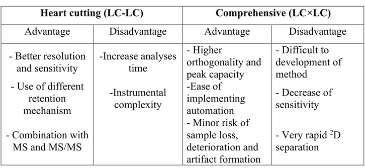
Pros and cons of heart-cutting and comprehensive approach are illustrated in Table 2.

Table 2: Pros and cons of MD-LC techiniques vs Conventional LC

Heart cutting (LC-LC) Comprehensive (LC×LC)

Advantage Disadvantage Advantage Disadvantage

- Better resolution and sensitivity -Increase analyses time - Higher orthogonality and peak capacity - Difficult to development of method - Use of different retention mechanism -Instrumental complexity -Ease of implementing automation - Decrease of sensitivity - Combination with MS and MS/MS - Minor risk of sample loss, deterioration and artifact formation - Very rapid 2_D separation

2.2 Theoretical aspects

The theoretical aspects that explained the advantages of the multidimensional separation have been developed much later than the first published work.

Initially, Connors [20] assumed that the distribution of spots on a 2D-TLC plate could be modeled according a Poisson distribution of data on each retention axis. The theory was based of the equations that related the number of chromatographic systems needed to separate a specific number of compounds. The challenge of this work was to find separation systems that are not correlated. Due to the system employed, that doesn’t base on the resolving power viz efficiency or the number of theoretical plates, it can't

(37)

apply for complex bio-separations. Further, Martin et al. [21] continued this study and offered a modern theoretical approach, that was further clarified in the modern years by Davis and Blumberg [22].

Finally, the most important theoretical aspects to consider in MD-LC are: peak capacity, orthogonality, resolution, sampling frequency, dilution factors and limit detection which will be discussed later.

2.2.1 Peak capacity

The reason of using multidimensional techniques is due to a better separation of the components than of a conventional method. The quality of separation can be evaluated by the peak capacity, this value was defined for the first time by Gibbings [23] in one-dimension, it corresponds to the maximum number of peaks separable in a specific part of the space. Few years later, the concept was introduced to multidimensional technique by Guiochon et al. [24,25] and Giddings [26,27]. The peak capacity in 2D separation is similar or slightly lower than the sum of peak capacities of each dimension. In particular, the 2D peak capacity is correlated to the separation mechanisms, if the systems are orthogonal the value of the peak capacity is higher. In the first concept of peak capacity [23], Gibbings described the equation for an isocratic condition:

0₁= 1 + √4

567ln : ;!<=

;_" <=> (1)

with N the efficiency, RS the resolution and ?₌ and ?_@ the retention factors of the first

and the last eluting components. The value of RS corresponds on the aim of the

(38)

For the gradient mode, the peak capacity is generally higher than the isocratic analysis, considering that the bandwidths (wi) are narrower. In the eqs. (2) and (3) are presented

the general formula to calculate the gradient peak capacity.

0₁= 1 + A#

B (2)

where, tg is the gradient run time and C is the average peak width (four or eight time

the value of the standard deviation of a peak).

0₁= A! _BD A" (3)

with E₌and E_@ correspond the retention times for the first and the last eluted peaks, respectively.

In the Eq. (2) the entire gradient run time is considering, instead unused space at both end part of the chromatogram is taken into account when using (3).

It is important to highlight these equations are valid when the peak width pattern over the entire chromatogram is very similar. When the operating conditions changing during the analysis, more complex procedures for the determinate the peak width C are used to calculate the peak capacity. There are several theories and equations for the calculation of the peak capacity, and it is very difficult to choose the correct formula. The key point is based on the theoretical value calculated by multiplication peak capacities of the separate dimensions.

0_{1,AGHIJHAK1LM} = 0= ₁× O0₁ (4)

where =n_P and On_P is first- and second peak capacity, respectively. This eq. does not consider the deleterious effects due to the modulation processes as well as possible

(39)

0_1,QJL1AK1LM OR ₌ !S% × S& % T= < U.UW × X '% (%& ! '# ! Y & (5)

the parameter Ot_P is the time of separation in 2_{D, it is the same as the modulation time,}

instead =E_[ is the 1_{D gradient time. In this eq. is including the parameter <β> that}

taking into account undersampling.

But, to obtain a realistic peak capacity it is important to evaluate possible peak distribution along in the 2D space with to aim to estimate 2D coverage, the orthogonality degree (A0) must be included in the final peak capacity (also known as

effective). 0_{1,H@@H1AK\H ] S} %,*+,%'-%,. &/ × #_^ OR ₍₆₎

2.2.2 Orthogonality

The major challenge in using the multidimensional peak capacity is to discover different set-ups that can spread the compounds across the separation space. It is possible, when the separation mechanism of the two columns is different or uncorrelated. The meaning of orthogonality is showed in Fig. 4 (a-b). where a comparison of NP × RP and NP × RP set-up is reported. Low correlation (high

orthogonality) is showed in the Fig. 4c for the separation of lemon oil where compounds are randomly distributed over the entire chromatogram space. On the contrary in Fig. 4d, the separation of steroids occurred in the linear mode. Due to the importance of the concept of orthogonality, different studies based of the mathematical point have been made.

(40)

Figure 4. Representation of orthogonality in comprehensive LC. (a) Low correlation, high

orthogonality; (b) high correlation, low orthogonality. Practical examples from reference [1]: (c) NP-LC×RP-LC separation of lemon oil. (d) RP-NP-LC×RP-LC separation of steroids.

Liu et al. [29] proposed a geometric study to factor analysis in which a correlation matrix was developed from the solute retention parameters. The area of 2D space covered by the peaks was calculated for the orthogonality and then was used as a subtraction factor applied to the theoretical peak capacity in order to obtain the real value. [1]

(41)

Slonecker et al. [30-31] have studied the orthogonality by terms as informational similarity (IS) which is a measure of the global solute crowding and percentage of synentropy (PS) based on the amount of a cross-information.

Gilar et al. [32] explained orthogonality like the normalized area covered by each peak, after the normalization step of the retention time values obtained in both separations and correlated to the peak area of each blob.

The concept of orthogonality was resumed in 2014 by Camenzuli and Shoenmakers [33]. This procedure regards the distribution of each peak along the virtual lines that cross the 2D plot forming an asterisk, where Z- , Z+ (diagonal lines of the asterisk) and

Z1 , Z2 (vertical and horizontal lines). Z parameters explain the use of the separation

space in comparison of the correlated Z line, enabling semi-quantitatively diagnose areas of separation space where the sample constituents are plotted, reducing in practice orthogonality.

2.2.3 Resolution

The resolution for 2D separation presented by Peter et al. [34] was studied to calculate a resolution value and the separation quality for each set-up.

This parameter is calculated on the valley-to-peak ratio between two close peaks (peak 1 and peak 2), three maximum intensities are considered: the maximum of the peak 1 (max1) and peak 2 (max2), the highest point between the peaks (S) and the distance between max 1 and S, (d1,S) and the distance between max 2 and S, (d2,S).

__=,` = a(∆=_E

6=,`)O+ (∆OE6=,`)O (7)

__O,` = a(∆=_E

6O,`)O+ (∆OE6O,`)O (8)

being ∆=_E

(42)

Intensity g is calculated by:

d = e!,0G1,2&<e&,0G1,2!

e_!,0<e_&,0 (9)

where ℎ_gLh= and ℎ_gLhO are the maximum height of the peaks 1 and 2. The valley-to-peak ratio (V) is measured as:

i = @

[ =

([DG3)

[ (10)

Finally, resolution (Rs) is calculated as:

j_` = k=

O l0 m =Dn

O o (11)

2.2.4 Sampling frequency

Sampling frequency or modulation periods is fundamental to maintain the 1_D

resolution in a comprehensive configuration. For example, when sampling value is larger than the peak widths obtained in 1_{D it follows a big reduction in the resolution}

in the first dimension resolving power, due to the mixing prior to the transfer into the second dimension. In particular, the peaks that were partially separated by the first column are collected in the same fraction and the partially separation is completely lost. To avoid this situation, a fast second dimension analyses is necessary. Consequently, the time for the separation in the second dimension is reduced and hence, the peak capacity of the second column is very low. Instead, the flow rate in the first dimension is very slow, below the Van Deemter’s optimum value, in order to get

(43)

the widest possible peaks. In this way, the number of sampling for the primary peak is greater, but the main drawback is a reduced peak capacity in the first dimension. In this regard, Murphy et al. [17] studied the effect of the sampling rate on the first dimension peak width through a modeled Gaussian peak as a histogram profile of the average concentration in each sampling period. Briefly, their theoretical and experimental data proved that is necessary three sampling along the peak, calculated a 8p peak width for each peak. This value is valid when the sampling is “in-phase” therefore the sampling should start at the beginning of the peak. In the experimental analysis, this is very complicated and so a minimum value of four sampling is recommended. In addition, most studies are based on 4 p peak widths values.

Seeley [35] investigated the sampling frequency for the modulators with several duty cycles for a theoretical study. In particular, when the effluent of the first dimension is collected in the entire sampling period, the duty cycle is equal to unity. This is the case when an interface of a two-position/8- or 10 ports switching valve equipped with two sampling loops is used, on the contrary when is used only one storage loop the duty cycle is less than 1.

Seeley also introduced the (average) peak broadening factor p* (<p ∗>) by detailing parameters as sampling period r_s and sampling phase t. The parameter r_s is calculated by the sampling time ts or modulation period and 1p of the first dimension peak, and t

is the manner in which the primary peak is cut into fractions. The difference time between the center of the sampling cycle nearest to the peak maximum and the peak maximum, divided by the sampling period is the sampling phase (t). When the peak maximum was center in one of the sampling periods and for low duty cycles, the peak broadening greatly was reduced. Usually, for the most comprehensive separations the duty cycle is 1 and the peak broadening is independent of t. In conclusion, Seeley has deduced the same conclusion as Murphy et al.

Other important applications were introduced by the group of Carr [28, 36, 37], these are based on the effect of undersampling on the whole chromatogram, in contrast to all previous studies where focused on just a single couple of peaks. A new parameter based