Discussion Papers
Collana diE-papers del Dipartimento di Economia e Management – Università di Pisa
Giulio E
CCHIA
Francesca G
AGLIARDI
Caterina G
IANNETTI
Social Investment and youth labour market
participation: a EU regional analysis
Discussion Paper n. 236
2
Discussion Paper n. 238: September 2018
Authors:
Giulio Ecchia, Department of Economics, University of Bologna
Francesca Gagliardi, Department of Economics and Statistics, University of Siena
Corresponing author: Caterina Giannetti, Deparment of Economics and Management, University of Pisa Email: [email protected]
©
Giulio Ecchia, Francesca Gagliardi, Caterina GiannettiLa presente pubblicazione ottempera agli obblighi previsti dall’art. 1 del decreto legislativo luogotenenziale 31 agosto 1945, n. 660.
Si prega di citare così:
Ecchia et al (2018), “ Social Investment and Youth labour market participation: a EU regional analysis”, Discussion Papers del Dipartimento di Economia e Management – Università di Pisa, n. 236 (http://www.ec.unipi.it/ricerca/discussion-papers.html).
3
Discussion Paper n. 236
Giulio E
CCHIA
Francesca G
AGLIARDI
Caterina G
IANNETTI
Social Investment and youth labour market
participation: a EU regional analysis
Abstract
In this paper, we first rely on small area techniques to derive from EU-SILC survey new indicators of compensatory and investment policies at regional level. While compensatory policies have mainly the goal of protecting individuals from “old” risks (e.g. old-age), investment-related social policies tend to focus more on “new social risks” (i.e. skill deficits). We rely on these new indicators to perform a data-driven SVAR analysis to investigate the casual relationships between youth labour market outcomes and these two types of spending. Our results support the view that investment policies are more effective for tackling new social challenges.
Keywords: small area techniques, investment policies, compensatory policies, SVAR analysis; ICA JEL: C18, C54, E02
The author would like to thank Kevin Albertson, Marco Capasso and Alessio Moneta for useful comments and suggestions, and Alessio Moneta for providing R codes. This project has received funding from the European Union's Horizon 2020 research and innovation programme under grant agreement No 649189, "Innovative Social Investment: Strengthening communities in Europe" (InnoSI)
1 Introduction
Since its inception, the EU has experienced robust convergence in terms of GDP per capita. How-ever, even though there was a convergence process at the country level, the convergence at the re-gional level has been much weaker. In particular, there are still some countries exhibiting rere-gional divergence or sustained North-South (or West-East) divides (Monfort[2008],Wunsch[2013]). That means, for example, that there tends to be much higher negative correlation between GDP and unemployment within countries than across countries. However, both mainstream and heterodox theories cannot explain the existence of these different regional trajectories and the weakness of the convergence processes among them (Iammarino et al.[2018]).
From an empirical perspective, this obviously raises the question about the role of the different policies adopted in the last years, both at European and country level (Wunsch[2013]). In this regard, in many European countries, several studies has documented a transition from the tradi-tional welfare states to a new investment state (e.g.Bonoli[2007],Ferragina et al.[2015],Obinger and Starke[2014]). In particular, it is possible to differentiate between two broad types of poli-cies: investment-related and compensatory policies (see, for example,Nikolai[2012]). Compensatory policies are mainly based on a contribution-financed social security with the goal of protecting individuals from “old” risks, such as unemployment and old-age. Investment-related social poli-cies tend to focus more on “new social risks” to overcome, through education and training, skill deficits that may emerge in post-industrial labour markets. Furthermore, these policies tend to reconcile work and family life. Thus, the focus is on investment in human capital as well as the provisions for the needs and the future of the younger generations. For example,Nikolai[2012] finds mixed evidence in support of a shift toward more social investment, with Continental and Southern European Countries being characterized by more spending for compensatory and less spending for investment-related policy (especially education).
However, without having expenditure data disaggregated at a regional level, it is quite impossi-ble to properly assess the impact of the two types of policies. As it has also been highlighted by the DG Regional Policy of the European Commission, in order to better target policy measures, there is an increasing need of social policy indicators developed at regional regional level (Verma
et al.[2013]). Therefore, the first contribution of our paper is to present new indicators of regional spending (which are comparable across regions and countries) which are derived through the cu-mulation methodology applied to the EU Statistics on Income and Living Conditions (EU-SILC) dataset (seeBetti et al. [2012]). In so doing, we will be able to derive for a subset of European countries, two regional indicators of compensatory and investment spending which are compara-ble across time and across countries.
The second contribution of our paper is to investigate the impact of these indicators on youth labour market participation within a Structural Vector Autoregressive (SVAR) framework. In par-ticular, we rely on a data-driven approach, recently introduced in the literature byMoneta et al.
[2013], which rely on Indipendent Component Analysis to identify structural parameters in SVAR (Gouriéroux et al.[2017],Lanne et al.[2017],Shimizu et al.[2006]). In particular, we adopt a more general identification scheme, called LiNGAM, i.e. Linear Non-Gaussian Acyclic Model (Shimizu et al.[2006]), to identify contemporaneous paramaters in order to identify the causal relationships among variables. Differently from standard methods (such as Cholesky decompositon), which necessarily requires either theoretical justification, this method has the great advantage to achieve identification directly from the data and statistical analysis alone.
While the low level of market participation of young people is not a new problem, the scale that has reached in the current economic crises is astonishing. For example, in some countries the youth unemployment rate has doubled or tripled since the onset of the recession (Mascherini et al.
[2012]). Therefore, traditional indicators of labour market participation, such as unemployment and youth employment rates do not adequately capture new “grey” area that represent market attachment in contemporary societies (Mascherini et al.[2012]). For this reason, we also investi-gate the effects of investment and compensatory policies on the share of young people who are disengaged from both work and education, usually indicated with the term NEETs (not in employ-ment, education and training). The needs to focus more on NEETs is now central in the European policy debate, and the term is explicitly mentioned in the Europe 2020 agenda as well as in the 2012 Employment Package “Towards a job-rich recovery” (Eurofond[2012]). In particular, at the Eu-ropean level, the term NEETs has caught the attention of policy markers as a useful indicators for monitoring the labour market participation and social situation of the young.
Our analysis of regional spending suggests that, even though the evidence is consistent with previ-ous analyses using national data to what concern the compensatory component (see, for example,
Hemerijck[2013],Heitzmann et al.[2015],Hemerijck[2017]), there is higher regional variation in the investment component, even within the same country. The results from our SVAR analysis also suggest that investment policies are more effective to reduce the level of NEETs and increase the level of youth employment.
In the following, we first describe how we derive our dataset. In particular, in section 2 we briefly review the main statistics on labour market participation of the young, which are currently avail-able at Eurostat, and the main issues related to data on regional expenditure. In section 3 we describe the cumulation methodology, and we apply it to EU-SILC in order to develop indica-tors of compensatory and investment spending at regional level, while in section 4 we rely on a recently developed econometric methodology (Moneta et al.[2013]) to investigate the effects of these types of policies on labour market outcomes. Section 5 concludes our argument.
2 Issues with regional data
In this section we describe the economic indicators of youth labour market participation we will use in our analysis (i.e. our outcome variables), and we discuss the main issues related to the collection of regional data on expenditure (i.e. our policy variables).
2.1 Regional Data on young people’s labour market participation
While NEETs and youth (un)employment are related concepts, there are important differences. In particular, unemployment rate measures the share of the labour population who are not able to find a job. More precisely, it is a measure of those who are out of work, but have actively looked for work in the recent past and is available for work in the near future. However, this measure does not take into account the “new risks”, that is it does not capture those who became discouraged and decided to stop looking for a job (Mascherini et al.[2012],Eurofond[2012]). This implies that the unemployment rate may stop falling even when a relevant number of individuals are at high risk of labour market and social exclusion. A similar remark can be made for youth
employment rate, which measure the share of the working age population (i.e. people aged 15 to 24) who is currently employed. In contrast, the NEETs captures the share of the young population currently disengaged from the labour market and education, namely unemployed and inactive young people not in education or training. More precisely, we have
Youth unemployment rate= Total young unemployed
Young Labour Force (1)
NEET rate= Total NEET
Young Population (2)
For this reason, to have an additional indicator for monitoring the situation of young people in the framework of the Europe 2020 strategy the European Commission (DG EMPL) agreed on a definition and methodology for a standardized indicator to quantify the size of the NEETs popu-lation among Member States. This indicator has been built by Eurostat using equation (2), and is available at Eurostat.1We report it in Table (1) as computed at NUTS1 level, along with measures for unemployment and employment of the young for the 15-24 age group.
INSERT TABLE (1) HERE
In particular, this table reports for each variable, in addition to the mean (µ) and the standard deviation (s) computed at country-level, the coefficient of variation (CV). This latter indicator is a normalized measure of dispersion defined as the ratio between the standard deviation and the mean (i.e. s
|µ| ). For a given standard deviation value, it thus indicates a high or low degree of
variability only in relation to the mean value. Since the coefficient of variation is a measure of relative variability which is unit-free (i.e. does not depend on the unit of measurement), it is often preferred to the standard deviation which has no interpretable meaning on its own. In particular, the CV indicators is among those indicators of s convergence, which is a term used to refer to a reduction of disparities among regions over time (seeMonfort[2008]).2
1More precisely, the numerator of the indicator refers to persons who meet the following two definitions: a) they are
not employed and b) they have not received any training or education in the four weeks preceding the survey.
2The concept of s convergence is strictly related to the concept of b convergence, which implies a catching up
For example, from Table (1) we can observe that high level of youth employment rates can be ob-served in Austria (AT), Denmark (DK), Finland (FI), the Netherlands (NL), and United Kingdom (UK). Conversely, young people seem particularly disengaged from the labour market in Slovakia (SK), Bulgaria (BG), Lithuania (LT), Italy (IT), Hungary (HU) and Greece (GR). Moreover, although there is not high variation in youth employment rate across European countries, there is a large variation in youth unemployment rate (with the CV being between 13-15%). The level of NEETs is also very different among EU countries.
However, as Figure (1) suggests, the EU-28 CV computed at NUTS1 level is increasing over time for all these measures. This suggests a divergence among EU countries in the level of unemploy-ment, employment and NEETs.
INSERT Figure (1) HERE
Finally, it is important to notice, that the increase in Regional disparities within EU as a whole does not prevent disparities from decreasing within each Member states (Monfort[2008]). For this reason, we also compute CV indicators for each Member State at regional level (where NUTS1 level data are available). However, even when we look at the regional variation between countries for the same variable, we can notice that for some countries, the regional variation can be very large: for example, in Italy and Portugal the CV is about 40%. The aim of the next sections will be to investigate how tcompensatory or investment-related policies affect these outcome variables.
2.2 Regional data on expenditure
Social policies that are defined as social investment policies are usually categorized according to three aspects (Heitzmann et al.[2015]):
1. Policies that help maintain or restore the capacity of labour market participants (e.g. old age pensions);
2. Policies that facilitate the entrance of new labour market participants (short-term unemploy-ment insurance; short-term maternity leave)
3. Policies that invest in the capacity of new labour market participants (elderly care, child care);
Unfortunately data on these dimensions are often not available at regional level and for several years. For these reasons, any attempt to examine the development of social investment across regions and countries often fails. Even if alternative approaches are available (e.g. De Deken et al.[2014]), because of data limitation, researchers largely end up with two categories, one for compensatory (i.e. the old risk categories) and another for social investment policies (i.e. the new risk categories).
In this analysis, we similarly distinguish between these two broad categories, but in addition to previous research we rely on data from EU-SILC survey to derive indicators at country regional level. The EU-SILC is a very rich survey on income and social condition collected at household (and individual) level under a standard integrated design by nearly all EU countries. As explained below, we rely on small area estimation (SAE) techniques to derive regional indicators of invest-ment and compensatory policies from EU-SILC survey (Betti et al.[2012]). More precisely, for each category of spending (investment and compensatory), we derive a series of indicators by comput-ing the average amount received per household at NUTS1 level. This an important contribution to previous studies, in which indicators of total spending where usually derived – at a country level – as a share of the GDP (see also Prandini et al (2015) on this issue). In particular, as described in the next section, we rely on cumulation technique (Betti et al.[2012],Verma et al.[2013]).
3 Cumulation Methodology
In order to better target policy measures, there is an increasing need of social policy indicators developed at regional regional level. For example, the DG Regional Policy of the European Com-mission is aiming to use regional level data to correctly identify regions with the highest propor-tion of people being poor or socially excludedCommission[2010]. However, regional level data, which is homogeneously gathered across countries, is often lacking.
For these reasons, EU-wide comparative datasets such as EU-SILC, even though primarily de-veloped to construct indicators at the national level, can serve as a unique source for generating
comparative indicators at regional levels through SAE techniques. Such methodologies have al-ready been proved to be successful to derive regional measures of poverty (Betti et al.[2012]Verma et al.[2013,2010],Marchetti et al.[2015],Betti et al.[2012]).
In particular, two types of measures can be constructed from national survey by aggregating in-formation on individual elementary units at the regional level:
1. average measures such as totals, means, rates and proportions constructed by aggregating or averaging individual values; and
2. distributional measures, such as measures of variation or dispersion among households and persons in the region.
In particular, we rely on the first type of measures, which are obtained by cumulating and consol-idating the information over waves of national sample surveys in order to obtain measures which permit greater spatial disaggregation. However, many measures of averages can also serve as in-dicators of disparity and deprivation when seen in the regional context: the dispersion of regional means is of direct relevance in the identification of geographical disparity (Verma et al.[2013]). To be able to compute spatial statistics through cumulation, the only information required is the strata identifiers from which individuals are sampled from. More specifically in our case, to cu-mulate over waves we need to know from which NUTS1 region the individuals were sampled. Unfortunately, this information is only available for a limited numbers of countries, namely: Aus-tria, Belgium, Bulgaria, Czech Republic, France, Greece, Hungary, Italy, Poland, Spain, Sweden, United Kingdom. Therefore, only for this group of countries, we were able to derive a an indicator of regional spending at NUTS1 level along with a measure of dispersion (i.e. the regional CV). For the remain group of countries, we were only able to derive country-level indicators from EU-SILC. Specifically, we proceed as follows. Given that we have the cross-sectional dataset of the EU-SILC survey for 9 consecutive years (from 2006 to 2014), the objective is to compute the cumulative average of a given measure y over 3 years, i.e. ¯yc
t.
We first construct for each year (i.e. for each EU-SILC wave) the yearly average relying on N individual observations (i.e. ¯yt = N1 ÂNi=1yi). Then for each year t, we estimate the required
statistic ¯yc
tas the one-year moving average over 3 consecutive years of the annual average ¯yt, that is
¯yc
t = ¯yt 1+ ¯y3t+ ¯yt+1 = 1t t
Â
j=1 ¯yj
However, to allow for more variability in our dataset, we only allow for one overlapping year across observations, relying therefore on 4 central years, i.e. we select ¯yc
2007, ¯yc2009, ¯yc2011, ¯yc2013.
3.1 EU-SILC Variable Selection.
As explained above our reference data is the EU-SILC survey, which provide us the necessary variables to compute indicators of compensatory and investment policies as in the current litera-ture. In particular, we rely on the following variables from EU-SILC data available from questions related to household gross income to derive the level of compensatory spending (in parentheses we report the EU-SILC number of each variable):3
1. unemployment benefits (PY090G): refers to (full o partial) benefits for benefits compensat-ing for loss of earncompensat-ings. It also includes early retirement, vocational traincompensat-ing, redundancy compensation, severance and termination payments;
2. old-age & survivors benefits (PY100G): refers to the provision of social protection against the risk linked to old age (e.g. old age pensions, care allowance) or to the loss of the spouse (survivor’s pension, death grant);
3. sickness benefits (PY120G): refers to benefits that replace in whole or in part loss of earnings during temporary inability to work due to sickness or injury (e.g.. paid sick leave);
4. disability benefits (PY130G): refers to benefits that provide an income to persons impaired by a physical or mental disability (e.g. disability pensions, care allowance);
Similarly to derive the level of investment policies, we select the following variables:
3Seehttp://ec.europa.eu/eurostat/web/income-and-living-conditions/methodology/list-variables
1. education-related allowances (PY140G): refers to grants, scholarships and other education help received by students;
2. family/children allowances (HY050G): refers to benefits that provide financial support to bringing up children and relatives other than children (e.g. Birth grant, Parental leave bene-fits, earning-related payments to compensate loss of earnings);
3. housing allowance (HY070G/HY070Y)): interventions that help households meet the costs of housing (e.g. rent benefits granted to tenants);
More generally, both groups of variables are defined as current transfers received by the household during the reference period, through collectively organized schemes, or outside such schemes by government units and Non-Profits Institutions Serving Households (NPISHs). Therefore, this definition includes the value of any social contributions and income tax payable on the benefits by the beneficiary to social insurance scheme or tax authorities. To be included in these groups of variables, the transfer must meet two criteria: i) the coverage is compulsory; ii) it is based on the principle of social solidarity. Importantly, the social benefits included in EU-SILC, with the exception of housing benefits, are restricted to cash benefits.
3.2 Regional Spending Results
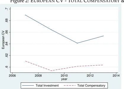
We now apply the cumulation methodology to obtain – for each one of the selected variable de-scribed in the previous section – the NUTS1 level average. We then categorized all these variables into the two groups of compensatory and investment variables. The national average over 4 years is reported in Table (2), while in Figure (2) we report the CV indicators computed at European level (EU28) for both total investment and total compensatory variables.
INSERT TABLE (2) HERE INSERT FIGURE (2) HERE
First of all, we observe that there is a remarkable difference in the CV for total investment across Europe, being the CV almost 0.70 in 2007 and much larger in comparison to the CV for total
compensatory. However, we also observe that even though the difference for total investment remains higher than for total compensatory, there is a tendency for a reduction in the period 2007-2013. In line with Nikolai (2012) andObinger and Starke [2014], but relying on a very different dataset, we therefore find evidence for a s convergence in investment spending in Europe, while we observe a more stable pattern for total spending for compensatory policy.
In addition, we are able to compute indicators of regional variation in total spending within a group of European countries. As highlighted above, even if regional disparities decrease (or in-crease) when considering the EU as whole, it does not prevent disparities from increasing (or decreasing) with each Member states. The CV for total compensatory and total investment are re-spectively reported in Figure (3). While the regional CVs are much smaller than European CVs, we can similarly observe a similar pattern. That is, we also observe within countries a much smaller level of the CVs for compensatory policy (being always smaller than 0.15), while we observe a larger level of CVs for total investment (being in some cases around 0.40). However, even in this case, we observe a tendency for a s convergence, with the only exception being Bulgaria and Greece for total investment.
INSERT FIGURE (3) HERE
4 SVAR Analysis
In this section we use the dataset described in the previous sections to estimate a structural vector autoregressions (SVAR) model to identify casual relationships among our variables of interests. SVAR models are among the most prevalent tools in empirical economics to analyze casual effects (seeStock and Watson[2007]). The underlying set-up is the reduced-form Vector Autoregressive (VAR) model, which is a system of equations for a vector of k variables, in which each variable is made dependent on its own past values, the lagged values of the other variables, and a specific white-noise error term. This model can be easily estimated through standard regression methods (e.g. OLS), since all the regressors are pre-determined variables. The reduced-form VAR model, however, does not provide enough information to study the causal relationships among the vari-ables and is typically used for the sake of descriptive statistics and forecasting only. It does not
provide the structural information because it typically omits the possible influence of contempo-raneous values and it delivers error terms that are usually correlated (across variables), so that they cannot be interpreted as genuine shocks affecting the system or as exogenous interventions. Thus, the estimated parameters cannot be used to predict the effect of an intervention. Structural analysis is instead the objective of SVAR models, which add structural information to the VAR (i.e. they solve the identification problem) so that one can recover the causal relationships existing among the variables under investigation. The common approach is to derive this structural information from economic theory or from institutional knowledge related to the data generating mechanism (Stock and Watson[2007]).
In the following, we instead rely on a more data-driven approach recently developed in the liter-ature byMoneta et al.[2013] to fully identify the SVAR model. In particular,Moneta et al.[2013] have shown that if the estimated (reduced-form) VAR residuals are non-Guassian, one can exploit higher-order statistics of the data and apply ICA, i.e. Independent Component Analysis (Hyvärinen et al.[2001]). This method has therefore the great advantage of avoiding subjective choices and theory-driven considerations to estimate SVAR model. ICA methods for the statistical identifica-tion of SVAR models have also been proposed byGouriéroux et al.[2017] andLanne et al.[2017]. In the following we briefly review this methodology. For interesting applications of this method seeBrenner et al.[2017],Guerini and Moneta[2017],Ciarli et al.[2018],Herwartz[2018].
4.1 Independent component analysis and SVAR identification
We can denote by Yt = (Y1t, .., Ykt)0the values at a particular time t of a multiple time series dataset composed of k variables collected for T periods. A simple - but useful - way of representing the data generating process is to model the value of each variable Yktas a linear combination of the previous values of all the variables as well as their contemporaneous values:
Yt =BYt+G1Yt 1+...+GpYt p+et (3) where the diagonal elements of the matrix B are set equal to zero by definition and where et rep-resents a vector of error terms with covariance matrix E(ete0t) = Âe. Since these terms represent
the structural shocks affecting the system, we can assume that they are uncorrelated, so that Âeis a diagonal matrix and that e1t, . . . , ektare mutually independent. Uncorrelatedness of the shocks is a standard assumption in the SVAR literature, while independence is usually not explicitly as-sumed (also because in a Gaussian setting it is equivalent to uncorrelatedness), but is implicit in many discussions about the economic interpretations of the shocks (Kilian and Lütkepohl[2017]). The model in the standard SVAR form c an be equivalently written as
G0Yt =G1Yt 1+...+GpYt p+et (4) where G0 = I B. Since variables are endogenous in (3) and (4) this model cannot be directly estimated without biases. It is typical therefore to derive and estimate the VAR reduced form
Yt =G01G1Yt 1+...+G01GpYt p+G01et
Yt=A1Yt 1+. . .+ApYt p+ut (5)
which can be straightforwardly estimated through standard regression methods (e.g. OLS regres-sions).
The problem of identification is therefore the problem of finding the appropriate G0. Traditionally, this problem is solved by choosing G0 on the basis of a Cholesky factorization of the estimated matrix Su of covariance among the reduced-form residuals ut. This imposes a recursive struc-ture among the variables (G0 results lower triangular) and yields orthogonal structural shocks. A problem with this method, however, is the Cholesky factorization is dependent on the chosen order of the variables(Y1t, . . . , Ykt)0 in Yt. A re-ordering of the variable will produce a different Cholesky factorization and a different recursive causal chain among the variables. Thus, this way of proceeding can only be used when the recursive ordering implied by the identification scheme is supported by theoretical or institutional knowledge.
The method proposed byMoneta et al.[2013] instead, applies a search procedure based on ICA, which is able to find, on the basis of data and statistical analysis alone, the appropriate matrix G0
that relates the vector of the structural shocks et such that G0ut =et. ICA starts from the consid-eration that utare mixtures, i.e. linear combinations, of latent sources, or independent components,
et. It is crucial for ICA, that etare independent and non-Gaussian. Hence, G0and etare recovered by searching the linear combinations of ut that are least statistically dependent in the style of un-supervised statistical learning typical of the machine learning research (Hyvärinen et al.[2001]), where the measure of statistical dependence used in this context is mutual information. Non-Gaussianity here goes hand in hand with independence: if etare non-Gaussian and independent, any linear combination of them will be closer to a Gaussian distribution (see central limit theo-rem). Then ICA can also be seen as method which searches for linear combinations of the data that maximizes non-Gaussianity. Hyvärinen et al.[2001] show that searching for linear combina-tions of ut that are maximally independent (or least dependent) is equivalent to searching for et that are maximally non-Gaussian (using the notion of negentropy).
ICA alone, however, leaves undetermined the scale, the sign and order of the latent sources or structural shocks. In other words, G01 is identifiable up to a column permutation and the mul-tiplication of each of its diagonal elements by an arbitrary non-zero scalar (seeGouriéroux et al.
[2017]). While the scale indeterminacy can easily solved by rescaling the column of G 1
0 so that all the shocks have unit variance, to solve indeterminacy of the order of the column of G 1
0 we need to make further steps, hinging on a further assumption.
Hence, in the following we rely on a more general identification scheme, called LiNGAM, i.e. Lin-ear Non-Gaussian Acyclic Model (Shimizu et al.[2006],Moneta et al.[2013]), which incorporates ICA (more specifically, the FastICA algorithm by Hyvärinen et al. [2001]) in the first step, and then solves its indeterminacy problems by making the further assumption of recursivenes. This assumption means that, given a particular contemporaneous causal order of the variables, the G0 matrix can be transformed in a lower-triangular matrix and the contemporaneous causal order of the variables can be represented as a directed acyclic graph (Moneta et al.[2013]).4
It is important to notice that with LiNGAM the specific ordering of the variables that produces a lower triangular matrix ( G0 ) is found out directly from the data, while in the Choleski scheme is given a priori. LiNGAM recovers the specific ordering of the variables that produces a lower
4For other methods based on a-theoretical search procedures based on normality see e.g. Swanson and Granger
triangular matrix (G0) from the output of ICA. Since, under recursiveness, both G0 and G01 con-tain k(k 1)/2 zero entries, LiNGAM search for the unique permutation of G01which has
non-zeros on the main diagonal. Since ICA estimates G01with measurement errors, LiNGAM actually searches the permutation which makes G01the closest as possible to lower triangular.
To summarise, our procedure is based on the following assumption: 1. the shocks(e1t, .., ekt)are non-normally distributed;
2. the shocks(e1t, .., ekt)are statistically independent;
3. the contemporaneous causal structure among (Y1t, .., Ykt)is recursive, that is there exists a re-ordering of the variables such that G0is lower triangular; the appropriate ordering of the variables, however, is not known to the researcher a priori.
The first assumption can be easily tested in the data. The second assumption is consistent with the interpretation of the elements of et as structural shocks, i.e. exogenous processes that affect each variable of the system at each time in an independent way. In other words, this assumption means that any shock affecting, for example, the level of compensatory spending will not simultaneously affect the shock affecting the level of investment spending (although it can of course also affect the variable level of investment spending). This assumption, however, cannot be directly tested. Finally, the third assumption is necessary to perform the LiNGAM method. While it has the dis-advantage of relying on a lower-triangular scheme, LiNGAM has the clear dis-advantage compared to other algorithms of providing a complete identification of G0 (with the entire causal graph of the contemporaneous structure) directly from the data.
4.2 Results
Relying on NUTS1 level data, we apply the ICA method to explore relationship between the level of compensatory and investment spending on the level of NEETs, unemployment and employ-ment of the young. The results from this SVAR analysis are reported in Table (3) and can be interpreted in a causal way. The column variables are the cause, while the raw variables are the effects. The model is estimated in differences as variables are highly persistent. To validate the
use of this methodology, we conducted checks on the empirical distributions of the VAR residuals
(u)– as well as the results of the Shapiro-Wilk and the Jarque-Bera tests for normality; for all the
variables, the tests rejects the null hypothesis of normality for the residuals (results are available upon request).
We start by observing the contemporaneous effects from Table (3). It must be noted that the struc-ture of this table reflects the recursive strucstruc-ture implied by the ICA method. After re-ordering the variables (i.e. NEETs, Employment Young, Log Compensatory, Unemployment Young, Log GDP and Log Inv), a lower triangular structure emerges.5 For our purpose, this matrix is not very informa-tive as it implies zero contemporaneous impact of investment spending on any of our variables of interests, i.e. (un-)employment and NEETs, and a significant impact of compensatory spending on GDP.
We therefore resort to an impulse-response function (IRF), which describes over a specified time horizon the evolution of the variable of interest after a (one-standard deviation) shock to another variable in the system. In Figure (4) we report the IRFs which are related to our policy variables, i.e. the total amount spent in compensatory and investments policies per household. The first thing to notice is that a one shock deviation in the level of compensatory spending per household (about 1000 Euro) will slightly and significantly increase up to 0.2% the level of NEETs, although this effect tends to become zero and statistically insignificant within three years. On the contrary, a shock in the level of investment spending per household (about 1350 Euro) will slighlty reduce the level ofNEETS(about -0.2%) although this effect tends to become zero and statistically insignificant over time.
INSERT FIGURE (4) HERE
We then observe that the same shock in compensatory spending has no significant effect on em-ployment, while the shock in investment spending has a small positive and significant effect on it (up to 0.4%). This latter effect tends to disappear after few years. Finally, we observe that the shock in compensatory spending has also a significant and positive effect on unemployment (up
to 0.6%), while the shock in investment spending has a significant, although smaller, negative effect on it (up to -1%).
Overall, these results suggest that shocks in the level of total investment spending lead to more positive economic outcomes, while the opposite is true for total compensatory.
5 Conclusions
As it has been already highlighted, both in the literature and at the institutional level, the regional dimension does matter. There are strong differences across regions in EU, but also inside individ-ual countries. Therefore, in order to better target policy measures, there is an increasing need of social policy indicators developed at regional level. Moreover, since young people paid the high-est price during the global economic crises, there is also a renewed sense of urgency to integrate them into the labour market and into the education system. Our paper offers contributions in both respects: we first construct new indicators of regional spending to then investigate their impact on new indicators - such as NEETs - of youth labour market participation.
In particular, we relied on Small Area Estimation techniques, as applied to the EU-SILC survey, to develop new indicators of compensatory and investment spending at NUTS1 level. These methodologies have already been proved to be successful to derive regional measures of poverty (Verma et al. [2013],Betti et al.[2012]). Interestingly, by looking at these measures, we can ob-serve across EU Member States regional convergence of compensating expenditure, and a milder of social investment.
We then used these new regional indicators of spending in combination with a recently developed SVAR approach (Moneta et al.[2013],Shimizu et al.[2006]) to investigate the casual relationships between labour market outcomes and different types of spending. While relying on Independent Component Analysis, this method has the great advantage of avoiding subjective choices and theory driven considerations to estimate SVAR model (Gouriéroux et al.[2017],Lanne et al.[2017]) Our main result suggests that social investment policies strongly differ across EU regions but can be more effective to enhance labour market outcomes of the young. This has an important policy implication as youth employment remains the crucial node to sustainable economic and social
References
Gianni Betti, Francesca Gagliardi, Achille Lemmi, and Vijay Verma. Subnational indicators of poverty and deprivation in europe: methodology and applications. Cambridge Journal of Regions, Economy and Society, 5(1):129–147, 2012.
Giuliano Bonoli. New social risks and the politics of post-industrial social policies. In The politics of post-industrial welfare states, pages 21–44. Routledge, 2007.
Thomas Brenner, Marco Capasso, Matthias Duschl, Koen Frenken, and Tania Treibich. Causal re-lations between knowledge-intensive business services and regional employment growth. Re-gional Studies, pages 1–12, 2017.
Tommaso Ciarli, Alex Coad, and Alessio Moneta. Exporting and productivity as part of the growth process: Results from a structural var. 2018.
European Commission. Europe 2020: A strategy for smart, sustainable and inclusive growth. Working paper European Commission, 2010.
Johan De Deken et al. Identifying the skeleton of the social investment state: defining and mea-suring patterns of social policy change on the basis of expenditure data. Reconciling work and poverty reduction. How successful are European welfare states, pages 260–285, 2014.
Eurofond. Neets: Young people not in employment, education or training: Characteristics, costs and policy responses in europe. Publications Office of the European Union, Luxembourg, 2012. Emanuele Ferragina, Martin Seeleib-Kaiser, and Thees Spreckelsen. The four worlds of welfare
reality: social risks and outcomes in europe. Social Policy and Society, 14(2):287–307, 2015. Christian Gouriéroux, Alain Monfort, and Jean-Paul Renne. Statistical inference for independent
component analysis: Application to structural var models. Journal of Econometrics, 196(1):111– 126, 2017.
Mattia Guerini and Alessio Moneta. A method for agent-based models validation. Journal of Economic Dynamics and Control, 2017.
Karin Heitzmann, Florian Wukovitsch, et al. Towards social investment and social innovation in eu member states? first observations of recent developments in austria. Technical report, Herman Deleeck Centre for Social Policy, University of Antwerp, 2015.
Anton Hemerijck. Changing welfare states. Oxford University Press, 2013. Anton Hemerijck. The uses of social investment. Oxford University Press, 2017.
Helmut Herwartz. Hodges–lehmann detection of structural shocks–an analysis of macroeconomic dynamics in the euro area. Oxford Bulletin of Economics and Statistics, 2018.
Aapo Hyvärinen, Juha Karhunen, and Erkki Oja. Independent component analysis. john willey & sons. Inc. New York, 2001.
Simona Iammarino, Andrés Rodríguez-Pose, and Michael Storper. Regional inequality in europe: evidence, theory and policy implications. Journal of Economic Geography, 2018.
Lutz Kilian and Helmut Lütkepohl. Structural vector autoregressive analysis. Cambridge University Press, 2017.
Markku Lanne, Mika Meitz, and Pentti Saikkonen. Identification and estimation of non-gaussian structural vector autoregressions. Journal of Econometrics, 196(2):288–304, 2017.
Stefano Marchetti, Caterina Giusti, Monica Pratesi, Nicola Salvati, Fosca Giannotti, Dino Pe-dreschi, Salvatore Rinzivillo, Luca Pappalardo, Lorenzo Gabrielli, et al. Small area model-based estimators using big data sources. J. Off. Stat, 31(2):263–281, 2015.
Massimiliano Mascherini, Lidia Salvatore, Anja Meierkord, and Jean-Marie Jungblut. NEETs: Young people not in employment, education or training: Characteristics, costs and policy responses in Europe. Publications Office of the European Union Luxembourg, 2012.
Alessio Moneta, Doris Entner, Patrik O. Hoyer, and Alex Coad. Causal inference by independent component analysis: Theory and applications*. Oxford Bulletin of Economics and Statistics, 75(5): 705–730, 2013. ISSN 1468-0084. doi: 10.1111/j.1468-0084.2012.00710.x. URL http://dx.doi. org/10.1111/j.1468-0084.2012.00710.x.
Rita Nikolai. Towards social investment? patterns of public policy in the oecd world. Towards a social investment welfare state, pages 91–116, 2012.
Herbert Obinger and Peter Starke. Welfare state transformation: Convergence and the rise of the supply side model. TranState Working Papers 180, University of Bremen, Collaborative Research Center 597: Transformations of the State, 2014. URL https://ideas.repec.org/p/ zbw/sfb597/180.html.
Shohei Shimizu, Patrik O Hoyer, Aapo Hyvärinen, and Antti Kerminen. A linear non-gaussian acyclic model for causal discovery. Journal of Machine Learning Research, 7(Oct):2003–2030, 2006. James H Stock and Mark W Watson. Introduction to econometrics. 2007.
V Verma, G Betti, and F Gagliardi. Robustness of some eu-silc based indicators at regional level. Eurostat Methodologies and Working papers, Luxembourg: Publications Office of the European Union, 2010.
Vijay Verma, Francesca Gagliardi, and Caterina Ferretti. Cumulation of poverty measures to meet new policy needs. In Advances in Theoretical and Applied Statistics, pages 511–522. Springer, 2013. Pierre Wunsch. Is the european integration machine broken. Intereconomics, 2(2013):78–83, 2013.
Figure 1: EUROPEANCV - NEETS,YOUNG EMPLOYMENT AND YOUNG UNEMPLOYMENT .3 .35 .4 .45 .5 European − 28 CV 2005 2010 2015 year Neets Unemployment Employment
Figure 2: EUROPEANCV - TOTALCOMPENSATORY& TOTALINVESTMENT SPENDING .6 .62 .64 .66 .68 .7 European CV 2006 2008 2010 2012 2014 year
Total Investment Total Compensatory
This figures reports the coefficient of variation (i.e. cv) for the European countries for Total Compensatory and Investment spending as derived in Table (3).
Figure 3: REGIONALCV - TOTALCOMPENSATORY AND IVESTMENT SPENDING a) Compensatory 0 .05 .1 .15 Regional CV − Tot. compensatory 2006 2008 2010 2012 2014 year AT BE BG CZ EL ES FR HU IT PL UK SE b) Investment 0 .1 .2 .3 .4 Regional CV − Tot. Investment 2006 2008 2010 2012 2014 year AT BE BG CZ EL ES FR HU IT PL UK SE
These figures reports the regional coefficient of variation (i.e. cv) for the European countries for Total Compensatory and Investment spending as derived in Table (3)
Figure 4: IMPULSERESPONSEFUNCTION 0 5 10 15 0.0 0.2 0.4 years Compensator y on neets 0 5 10 15 − 0.4 − 0.2 0.0 years In v estments on neets 0 5 10 15 − 0.4 − 0.2 0.0 0.2 years Compensator y on emplo yment 0 5 10 15 0.0 0.2 0.4 0.6 years In v estment on emplo yment 0 5 10 15 0.0 0.5 1.0 years Compensator y on unemplo yment 0 5 10 15 − 1.5 − 1.0 − 0.5 0.0 years In v estment on unemplo yment
Table 1: (U N ) EM P L OY ME NT R A T E Y OU N G (15-24) AN D N EE T S Employment rate young Country Mean Std CV Reg. CV AT 53.003 4.956 0.094 0.105 BE 23.406 5.251 0.224 0.258 BG 23.005 2.503 0.109 0.103 CY 32.991 5.237 0.159 . CZ 26.691 1.363 0.051 . DE 45.011 4.797 0.107 0.093 DK 60.036 4.665 0.078 . EE 31.309 2.890 0.092 . EL 19.994 6.648 0.332 0.145 ES 27.819 9.013 0.324 0.113 EU15 39.115 13.790 0.353 EU27 35.829 13.343 0.372 EU28 35.725 13.351 0.374 FI 41.673 1.918 0.046 . FR 29.078 4.821 0.166 0.155 HR 23.282 4.646 0.200 . HU 20.718 2.898 0.140 0.119 IE 38.591 9.640 0.250 . IT 21.956 7.577 0.345 0.312 LT 22.536 2.986 0.133 . LU 22.764 1.896 0.083 . LV 31.055 4.354 0.140 . MT 45.245 1.027 0.023 . NL 64.211 4.219 0.066 0.035 PL 24.842 2.800 0.113 0.089 PT 29.682 7.492 0.252 0.120 RO 24.114 2.375 0.098 0.088 SE 40.285 1.957 0.049 0.032 SI 32.764 4.213 0.129 . SK 23.391 2.953 0.126 . UK 49.699 5.931 0.119 0.098 Unemployment rate young Mean Std CV Reg. CV 9.828 2.954 0.301 0.342 26.072 9.712 0.372 0.432 21.688 6.374 0.294 0.269 20.000 11.176 0.559 . 16.433 3.485 0.212 . 12.113 4.408 0.364 0.286 10.850 2.769 0.255 . 18.783 7.168 0.382 . 38.517 15.420 0.400 0.107 36.169 15.010 0.415 0.160 20.483 11.937 0.583 . 20.901 10.852 0.506 . 21.009 10.912 0.520 . 20.367 2.926 0.144 . 24.206 8.759 0.362 0.307 34.817 8.676 0.249 . 20.872 6.614 0.317 0.288 19.217 8.945 0.465 . 30.587 13.024 0.426 0.401 20.825 8.786 0.422 . 16.858 2.340 0.139 . 21.900 8.586 0.392 . 13.892 1.979 0.142 . 9.185 2.790 0.304 0.113 26.369 7.403 0.281 0.136 31.995 12.542 0.392 0.183 21.933 3.579 0.163 0.150 22.342 2.350 0.105 0.052 15.583 3.696 0.237 . 28.917 5.172 0.179 . 16.813 4.563 0.271 0.179 Neets Mean Std CV Reg. CV 9.247 1.694 0.183 0.195 17.672 5.181 0.293 0.344 26.475 7.291 0.275 0.343 18.742 5.002 0.267 . 11.733 2.603 0.222 . 12.656 3.217 0.254 0.195 7.556 1.218 0.161 . 14.575 2.683 0.184 . 22.858 6.267 0.274 0.214 18.506 5.365 0.290 0.212 15.098 6.317 0.418 15.611 6.053 0.416 15.650 6.058 0.389 11.875 1.502 0.126 . 16.146 4.216 0.261 0.234 21.144 4.140 0.196 . 16.300 4.133 0.254 0.282 18.417 4.876 0.265 . 23.767 9.285 0.391 0.409 13.967 2.407 0.172 . 7.583 0.713 0.094 . 16.725 3.186 0.191 . 10.933 1.558 0.143 . 6.117 1.008 0.165 0.084 16.079 2.894 0.180 0.134 19.981 6.192 0.310 0.234 19.779 3.484 0.176 0.091 11.031 1.647 0.149 0.099 10.075 1.600 0.159 . 18.083 2.423 0.134 . 15.314 3.890 0.254 0.147
Table 2: DATA EU-SILC
This table reports the average (computed over 4 years: 2007, 2009, 2011, 2013) of the amount of euro an household received for each spending category. Data are derived from EU-SILC data through the cumulation methodology (see Section 3).
Old age & Sickness Unemployment Disability Total Education Family Housing Total
Survivors Compensatory Allowances Investment
AT 28963.660 2,133.389 3,983.593 12269.675 47350.318 2,395.584 5,024.067 1,540.396 8,960.046 BE 29985.481 6,882.746 8,393.498 9,745.557 55007.282 917.002 3,834.507 1,779.114 6,530.623 BG 2,050.337 295.416 506.534 889.021 3,741.309 282.490 487.128 157.721 927.339 CY 21591.830 1,997.840 6,341.432 8,135.511 38066.613 2,846.973 1,849.577 6,508.598 11205.148 CZ 5,481.341 966.027 955.940 3,276.192 10679.499 398.300 1,740.774 758.679 2,897.753 DE 21923.336 4,218.311 5,349.471 8,453.336 39944.454 3,580.148 3,757.179 2,303.338 9,640.665 DK 30574.877 4,678.608 8,326.608 19573.360 63153.454 5,292.157 3,032.879 2,398.943 10723.979 EE 4,559.260 321.178 1,244.568 1,769.974 7,894.980 708.651 1,492.453 558.574 2,759.678 EL 18139.462 2,019.569 2,904.287 6,043.221 29106.540 2,530.247 1,435.487 1,681.500 5,647.234 ES 19903.970 4,480.739 4,434.187 9,246.095 38064.990 1,497.090 2,735.697 2,222.783 6,455.570 FR 26178.656 3,014.565 6,113.630 6,409.401 41716.253 1,415.041 3,665.754 2,049.838 7,130.633 HU 5,480.686 385.845 958.555 2,322.598 9,147.684 614.371 1,536.951 207.887 2,359.209 IE 29213.996 2,549.636 8,027.722 7,420.527 47211.879 3,712.418 6,488.660 1,626.399 11827.477 IS 22798.902 8,001.309 4,240.782 14165.254 49206.247 2,463.721 3,163.754 1,791.669 7,419.144 IT 24419.023 . 3,870.974 6,591.035 34881.032 4,880.047 1,068.580 1,239.233 7,187.860 LT 3,186.222 412.592 845.385 1,774.985 6,219.184 430.034 1,422.239 142.519 1,994.792 LU 42241.571 13005.274 17458.672 19277.024 91982.543 4,268.158 8,058.280 1,853.503 14179.940 LV 3,977.220 536.278 855.717 1,574.061 6,943.276 507.077 802.829 215.703 1,525.609 NL 27844.778 4,981.020 8,273.349 14245.024 55344.171 2,818.128 1,967.597 1,810.706 6,596.431 NO 31123.304 5,802.989 6,474.943 17951.443 61352.680 2,447.223 5,948.912 2,287.293 10683.427 PL 7,615.036 828.574 1,472.368 2,364.762 12280.740 702.988 953.252 397.547 2,053.786 PT 11264.240 2,837.172 4,185.207 4,530.107 22816.727 2,339.191 770.973 436.278 3,546.441 SE 22602.767 2,388.459 6,088.357 10902.041 41981.625 2,996.206 4,810.426 2,421.003 10227.635 SI 14169.719 1,454.165 2,616.632 5,681.010 23921.527 1,625.774 2,203.959 699.723 4,529.455 SK 5,124.139 678.925 1,253.619 2,298.632 9,355.316 1,173.672 749.115 631.964 2,554.751 UK 19071.733 5,740.334 5,234.869 5,789.690 35836.626 4,764.372 4,074.775 4,947.629 13786.776
Table 3: V AR E STIMA TIO N : VA R IA B L E S IN D IFF E R E N C E (235 OB S -4 YE ARS ) The column-variables ar e the causes, while the row-variables ar e the ef fects. The B0-coef ficients give us the contemporaneous ef fects The B1-coef ficients pr ovides the ef fect of lagged variables (at time t-1 )on curr ent variable (at time t) Contemporaneous Ef fect (t): B0 Neets Employment Young Unemployment Young Log_GDP Log Compens. Log Inv Neets 0.000 0.000 0.000 0.000 0.000 0.000 Employment Young -0.547*** 0.000 0.000 0.000 0.000 0.000 Unemployment Young 1.469 *** -0.862 *** 0.000 0.000 0.055 0.000 Log_GDP -0.725 * 0.349 -0.324 0.000 0.334 ** 0.000 Log Compens. 0.705** -0.201 0.000 0.000 0.000 0.000 Log Inv -2.607 0.131 1.270 ** 1.258 *** 0.350 0.000 Lagged Ef fect (t-1): G1 Neets Employment Young Unemployment Young Log GDP Log Compens. Log Inv Neets -0.165 -0.113 -0.071 0.003 0.071 *** -0.021 Employment Young 0.063 0.100 -0.087 0.087 -0.091 0.056 Unemployment Young 0.355 -0.018 -0.198 -0.019 0.057 -0.031 Log_GDP 0.123 0.279 -0.205 -0.193 * 0.178 0.049 Log Compens. 0.083 0.189 0.231 0.310 ** 0.211 ** 0.028 Log Inv 2.269 ** 0.773 0.052 0.649 *** -0.044 -0.047