Climate change effects on <i>Durum wheat</i> (<i>Triticum durum</i> L.) in Mediterranean area

UNIVERSITÀ DEGLI STUDI DI SASSARI SCUOLA DI DOTTORATO DI RICERCA

Scienze e Biotecnologie dei Sistemi Agrari e Forestali e delle Produzioni Alimentari

Indirizzo : Produttività delle piante coltivate Ciclo XXVI

C

D

W

(T

L.)

M

Dr.ssa Silvia Baralla

Direttore della Scuola Prof. Alba Pusino

Referente di Indirizzo Prof. Rosella Motzo

Docente Guida Correlatori

Dr. Luigi Ledda Dr.ssa Roberta Farina Dr. Giovanni Di Genova

Sommario

Chapter 1 ... 8

1. Introduction ... 8

1.1. Background ... 8

European cereals production ... 8

Europe wheat production ... 8

1.1.1. Climate change impacts on wheat production ... 10

Climate change impacts on crop yield ... 10

Winter wheat production and Mediterrean climate ... 12

The main aspects of climate change on wheat production ... 12

Increasing of CO2 ... 14

Increasing of main temperature ... 14

Changing in variability of precipitation ... 16

Combination of the three factors ... 17

Impacts on biophysical, qualitative and socio economic aspects ... 19

Biophisical impacts on crops... 19

Biophisical impacts on environment ... 21

Pests, pathogenes and disease. ... 21

Socio-economic aspects ... 21

1.1.2 Modelling climate change ... 21

Crops model ... 21

Epic model ... 23

Introduction ... 23

Model description ... 25

GCMs and climate scenarios ... 34

1.2 Research question ... 38

1.3 Research objectives ... 39

Specific research objectives... 41

Chapter 2 ... 43

2.2.1 Oristano ... 46

Climatic baseline and future scenarios ... 46

Changes in climatic variables ... 47

2.2.2 Benevento ... 50

Climatic baseline and future scenarios ... 50

Changes in climatic variables ... 51

2.2.3 Ancona ... 53

Climatic baseline and future scenarios ... 53

Changes in climatic variables ... 54

2.3 Creation of the Epic model files ... 56

2.3.1 Soil data file ... 56

2.3.2 Weather data file ... 59

2.3.3 Management and crop data file ... 61

2.3.5 Control table ... 63

2.4 Experimental site description ... 64

2.4.1 Oristano ... 65

Observed climatic data ... 65

Soil data ... 67

Crop data and management ... 68

2.4.2 Benevento ... 70

Observed climatic data ... 70

Soil data ... 71

Crop and management data ... 72

2.4.3 Ancona ... 73

Observed climatic data ... 73

Soil data ... 75

Crop data and Management... 75

2.5 Statistical data analysis ... 77

2.6 Multivariate analysis ... 77

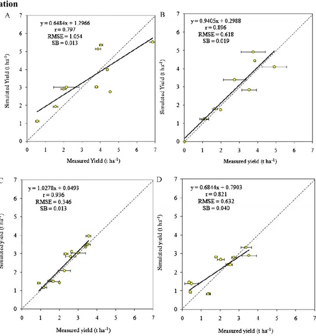
2.7 Running of the model: calibration and validation ... 78

2.7.1 Calibration ... 78

2.7.2 Validation ... 80

2.7.2.1 Oristano ... 82

2.7.2.2 Benevento ... 84 Validation ... 84 2.7.2.3 Ancona ... 86 Validation ... 86 Chapter 3 ... 87 Results ... 87

3.1 Climate change effects with different CO2 concentrations and crop stress ... 88

3.1.1 Oristano ... 88

3.1.2 Benevento ... 97

3.1.3 Ancona ... 105

3.2 Climate change effects with different CO2 concentrations and any crop stress ... 112

3.2.1 Oristano ... 112

3.2.2 Benevento ... 119

3.2.3 Ancona ... 126

3.3 Climatic change effects with same CO2 concentration and water crop stress ... 135

3.3.1 Oristano ... 135

3.3.2 Benevento ... 144

3.3.3 Ancona ... 153

3.4 Climatic change effects with same CO2 concentrations and any crop stress ... 162

3.4.1 Oristano ... 162

3.4.2 Benevento ... 171

3.4.3 Ancona ... 180

Chapter 4 ... 189

Discussion... 189

Epic model performance ... 189

4.1 Baseline climate effects ... 189

4.1.1 Vulnerabilities and climate impacts ... 189

4.1.1.1 Impacts on crop productivity ... 189

4.1.1.2 Impacts on the main variables: WUE, ET, GSP, WS and NS ... 190

4.3.1.1 Impacts on crop productivity ... 192

4.3.1.2 Impacts on the main variables: WUE, ET, GSP, WS and NS ... 193

4.4 Site comparison ... 194

6 Conclusion ... 200

ABSTRACT

This study work is carried out within the Agroscenari Project - Scenarios of adaptation to climate change in Italian agriculture, funded by the Ministry of Agriculture and Forestry with DM 8608/7303/08 of 7 August 2008. Within the different agricultural systems, this is the only work that considered rainfed agricultural systems with cereals as main crop, and specifically durum wheat. In the EU, too, cereals are the most widely produced crop. Cereals in fact account for over 50 % of some regions' UAA (Utilized Agricultural Area). Agricultural systems worldwide over the last 40-50 years have responded to the effects of the interacting driving forces of population, income growth, urbanization and globalization on food production, markets and consumption (Von Braun, 2007). To these forces can be added the twin elements of climate variability and climate change which have direct effects and serious consequences for food production and food security (Parry et al., 2004). Climate change is considered as one of the main environmental problems of the 21st century (Reidsma et al., 2010). It is definitively accepted that our climate is changing due to increased ―greenhouse gases‖ atmospheric concentrations and this change is expected to have important impact on different economic sectors (eg. Agriculture, forestry, energy consumptions, tourism, etc) (Hanson et al., 2006). In particular, for agriculture, such a change in climate may have significant impacts on crop growth and yield, since these are largely determined by the weather conditions during the growing season. Even in temperate regions, there are some early warning signs of climate change impacts on the yields of some major crops like wheat. A slower increase in grain yields compared to past decades has been reported in a range of countries, including Europe. Specifically climate change is projected to have a significant impact on temperature and precipitation profiles in the Mediterranean basin. The incidence and severity of drought will become commonplace and this will reduce the productivity of rain-fed crops such as durum wheat. The semi-arid regions, like Mediterranean area, are particularly sensitive to climate change for their characteristic climate conditions and increases in temperatures and in rainfall variability could generate negative impacts because high summer temperatures and water stresses already now limit crop production, according to the latest Assessment Report of the IPCC, Climate-Change 2007 (IPCC, 2007). Durum wheat is a rain-fed crop that is widely cultivated over the Mediterranean

seriously compromise durum wheat yields, representing a serious threat to the cultivation of this typical Mediterranean crop.

Different aspects of climate change, such as higher atmospheric CO2 concentration [CO2], increased

temperature and changed rainfall all have different effects on plant production and crop yields. In combination, these effects can either increase or decrease plant production and the net effect of climate change on crop yield depends on the interactions between these different factors (F. Ludwig, S. Asseng,2006). Higher CO2 almost always increases plant production (Amthor, 2001;

Poorter and Perez-Soba, 2001), but higher temperatures can, potentially, both increase or decrease grain yields (Van Ittersum et al., 2003; Peng et al., 2004). Assessments of climate change impacts on European agriculture (potential crop yield and biomass production) are examined using the Crop Growth Monitoring System (Supit et al., 2010) and suggest that in northern Europe, crop yields increase and possibilities for new crops and varieties emerge (Ewert et al., 2005; IPCC, 2007a; Olesen and Bindi, 2002).

This study was carried out to assess the effects of climate change on Durum wheat yields at field scale using a crop growth simulation model, EPIC and a climatic scenarios in order to simulate the crop response in future weather conditions. The climate scenarios were generated by General Circulation Models (GCM) and adapted to the field scale through downscaling processes. Specifically ECHAM 5.4 and RAMS were used. Understanding the consequences of long-term climate change is important for the agricultural policies and the choice of mitigation strategies. If consider wheat yields as main parameter influenced by climate change, drought conditions were the main factors limiting grain yields on clay soil in a Mediterranean-type environment, in particular this condition was observed for the Oristano site. The simulation experiments with long - term historical weather records suggest that environments characterized by low rainfall have negative impacts on crop growth: future climate change including higher temperatures and less rainfall will reduce grain yields despite elevated atmospheric CO2. In fact the CO2 positive effects

fail when we consider temperature and precipitations patterns in association with increased CO2

concentrations. Probably yields reduction, for Oristano site in the first set of results, was connected both to the falling of rain. The same simulation experiments carried out in the other two sites, Benevento and Ancona, showed a different situation: higher yields were observed in the future, maybe caused by higher future rainfall respect to the future condition. The results suggest priorization of adaptation strategies in the regions condisidered, including development of local cultivars of drought – and het resistant crop varieties, earlier planting to avoid heat stress, development and adoption of slower-maturing varieties to increase the grain filling period.

Chapter 1

1. Introduction

In terms of the area that they occupy and their importance in human and animal food supply, cereals constitute the largest crop group in the world.

In the EU, too, cereals are the most widely produced crop. European statistics on cereals encompass wheat, barley,maize, rye, meslin, oats, rice and other cereals, such as triticale, buckwheat, millet and canary seed. Cereals in fact account for over 50 % of some regions' UAA (Utilized Agricultural Area). These regions include the Balkan regions such as in Romania and eastern European regions, in particular in Hungary and Slovakia.

Cereal crops cover a relatively small proportion of the UAA in southern regions (except Basilicata) in certain Alpine regions, on the Atlantic coast of the Iberian peninsula and in the regions of northern Sweden, where this type of crop accounts for less than 10 % of the UAA.

Specifically, these regions include almost all regions of Portugal (except Lisboa region), and certain coastal areas of Spain (Galicia, Principado de Asturias, Cantabria, Comunidad Valenciana and Canarias) and Italy (Liguria).

The Alpine regions of Austria and Italy have areas under cereals of less than 10 % of their UAA. In certain regions in which the preference is for grassland and, in some cases, green fodder, a small proportion of the area is devoted to cereals. Those regions are in Belgium, France (Corsica, Limousin and the overseas department of Réunion), the Netherlands (Friesland, Overijssel, Gelderland, Utrecht and Noord-Holland), the whole of Ireland and the region of Mellersta Norrland in Sweden. Europe wheat production

Wheat (common and durum wheat) is by far the crop with the highest production in European agriculture. In 2007, wheat accounted for 46 % of cereal production in

statistics, only five regions do not produce wheat, namely Principado de Asturias in Spain, Valle d'Aosta/Vallée d'Aoste, Provincia Autonoma Bolzano/Bozen in Italy and Mellersta Norrland and Övre Norrland in Sweden.

In 2007, the EU produced 120 million tonnes of wheat (including 8.2 million tonnes of durum wheat), on a total area of 24 million hectares. Some 21 regions account for over half the wheat production in the EU (calculated without the figures for production in the Czech Republic, Greece and the United Kingdom, for which regional data are not available).

Of those 21 regions, 10 are in France, as follows (ranging from the highest production to the lowest): Centre (which accounts for 4.5 % of EU wheat production), Picardie, Champagne-Ardenne, Poitou-Charentes, Pays de la Loire, Nord Pas-de-Calais, Bourgogne, Haute-Normandie, Île-de-France and Bretagne. This makes France the biggest wheat producer in the EU. France harvested almost 33 million tonnes of cereal in 2007.

Germany, with 20.9 million tonnes, is the second biggest producer. It has eight of the 21 most productive regions, and they are as follows (from the largest producers to the lowest): Bayern (which accounts for 3.6 % of wheat production in the EU), Niedersachsen, Sachsen-Anhalt, Nordrhein-Westfalen, Mecklenburg-Vorpommern, Baden-Württemberg, Thüringen and Schleswig-Holstein.

It can, therefore, be said that the EU's wheat 'granary' is located in the northern half of France and Germany. The next 63 regions contribute 40 % of the EU's total production. These include all but three regions of Poland, which is the fourth biggest producer of wheat, after the United Kingdom (8.3 million tonnes) (Crop production statistics at regional level; Data from March 2009, most recent data: Further Eurostat information, Main tables and Database. http://epp.eurostat.ec.europa.eu/statistics_explained/index.php/Crop_production_statistics_at_regio nal_level).

Even in temperate regions, there are some early warning signs of climate change impacts on the yields of some major crops like wheat. A slower increase in grain yields compared to past decades has been reported in a range of countries, including Europe and India. For example, since 1990, winter wheat yields have been increasing at a significantly slower rate in France than over previous decades (Gate, 2009) and this change has foremost been attributed to an increased variability in climate (Gate 2007, 2009). By contrast, circumstantial evidence for climate-induced increasing grain yield of winter wheat (Triticum aestivum L.) from 1981 to 2005 at two locations in China has been challenged by a recent re-analysis (White, 2009).

1.1.1. Climate change impacts on wheat production Climate change impacts on crop yield

Agricultural systems worldwide over the last 40-50 years have responded to the effects of the interacting driving forces of population, income growth, urbanization and globalization on food production, markets and consumption (Von Braun, 2007). To these forces can be added the twin elements of climate variability and climate change which have direct effects and serious consequences for food production and food security (Parry et al., 2004). There is evidence for the effects of recent accelerated warming on many biological systems (IPCC, 2007).

Climate change is considered as one of the main environmental problems of the 21st century (Reidsma et al., 2010). It is definitively accepted that our climate is changing due to increased ―greenhouse gases‖ atmospheric concentrations and this change is expected to have important impact on different economic sectors (eg. Agriculture, forestry, energy consumptions, tourism, etc) (Hanson et al., 2006).

According to these premises, the assessment of cropping systems response to a warmer climate plays an important role for the evaluation of near future economic assets and the study of crop phenology response was indicated as a key stage for a better formulation of adaptation policies and options (Duchene and Schneider, 2005; Wolfe et al., 2005; Sadras and Monzon, 2006). 35

In particular, for agriculture, such a change in climate may have significant impacts on crop growth and yield, since these are largely determined by the weather conditions during the growing season. The changing weather patterns also affect crop production and the climate change impact on food security is widely debated and investigated (Miraglia et al., 2009). For example, Ludwig et al. (2009) investigated the impacts of the climate change on the wheat production in western Australia. Pathak et al. (2003) researched the decline/stagnation of the rice and wheat yields in the Indo-Gangetic Plains. Peltonen-Sainio et al. (2009) investigated cereal yield trends in Finland. Richards (2002) discussed the environmental challenges in Australian agriculture. Olesen and Bindi (2002) and Tubiello et al. (2000) elaborate on the consequences of climate change for European agricultural productivity 42.

Althought climate change may benefit crop production in northern latitudes above about 55°, where warmer temperatures may extend the growing season, in the developing world (especially sub – Saharan Africa) the projected changes are likely to have negative impact and will further complicate the achievement of food security (Fisher et al., 2001; Parry et al., 2004; Stern 2007).

Fischer et al. (2001) modelled the spatial variation in effects of climate change anticipated in 2050 on potential yields of rain-fed cereal crops worldwide and demonstrated that cereal producing

regions of Canada, and northern Europe and Russia might be expected to increase production, while many other parts of the world would suffer losses, including the western edge of the USA prairies, eastern Brazil, Western Australia and many, though not all, parts of Africa.

Overall, the results of this and subsequent work demonstrated that climate change would benefit the cereal production of developed countries more than the developing countries even if cropping practices evolved to allow more than one rain-fed crop per year (Fischer et al. 2002; 2005). 30 Winter wheat production and Mediterrean climate

The Mediterranean region, especially the Middle est and North Africa, ran out of renewable fresh decades ago. The region in one of the driest agricultural regions on earth, containing only 1% of the world‘s freshwater resources. The Mediterranean region in characterized by an extremely variable climate (Ceccarelli et al., 2007), with hot, dry summer and cool, wet winters, being the transition between dry tropical and temperate climates. This climate occurs on the west coasts of all continents between latitudes 30 and 45° due to global air circulation patterns. Mediterranean climate is associated with an area of about 2.76 million km2, corresponding to 2.3% of the Earth‘s land surface. The largest part is the Mediterranean region with 1.68 million km2 (60% of the total area of Mediterranean climate), followed by 0.61, 0.28, 0.13 and 0.06 million km2 _{for Western}

Australia, California, Chile and South Africa, respectively (Joffre and Rambal, 2002).48

The semi-arid regions, like Mediterranean area, are particularly sensitive to climate change for their characteristic climate conditions and increases in temperatures and in rainfall variability could generate negative impacts because high summer temperatures and water stresses already now limit crop production, according to the latest Assessment Report of the IPCC, Climate-Change 2007 (IPCC, 2007). Durum wheat is a rain-fed crop that is widely cultivated over the Mediterranean Basin. The major climatic constraints to durum wheat yield in Mediterranean environments are high temperatures and drought, frequently occurring during the crop‘s growth cycle (Porter and Semenov, 2005; Garcìa del Moral et al., 2003). As a consequence, projected climate changes in this region, in particular rising temperatures and decreasing rainfall (Gibelin and D´equ´e, 2003), may seriously compromise durum wheat yields, representing a serious threat to the cultivation of this typical Mediterranean crop.

climate change on crop yield depends on the interactions between these different factors (F. Ludwig, S. Asseng,2006). Higher CO2 almost always increases plant production (Amthor, 2001;

Poorter and Perez-Soba, 2001), but higher temperatures can, potentially, both increase or decrease grain yields (Van Ittersum et al., 2003; Peng et al., 2004)

Assessments of climate change impacts on European agriculture (potential crop yield and biomass production) are examined using the Crop Growth Monitoring System (Supit et al., 2010) and suggest that in northern Europe, crop yields increase and possibilities for new crops and varieties emerge (Ewert et al., 2005; IPCC, 2007a; Olesen and Bindi, 2002).

The main investigated crops are winter wheat, spring barley, maize, winter rapeseed, potato, sugar beet, pulses and sunflower.The changes appear in a geographical pattern. In Italy and southern central Europe, temperature and radiation change effects are more severe than elsewhere, in these areas potential crop yields of more than three crops significantly decreased. In the UK and some regions in northern Europe the yield potential of various crops increased (Supit et al., 2010).

In southern Europe, adverse effects are expected. Here, projected increases in temperatures and in water shortage reduce crop yields and the area for cropping. This will affect the livelihood of Mediterranean farmers (Metzger et al., 2006; Schröter et al., 2005). According to the IPCC definition, the extent to which systems are vulnerable to climate change depends on the actual exposure to climate change, their sensitivity and adaptive capacity (IPCC, 2001)

Specifically climate change is projected to have a significant impact on temperature and precipitation profiles in the Mediterranean basin. The incidence and severity of drought will become commonplace and this will reduce the productivity of rain-fed crops such as durum wheat (D. Z. Habash, Z. Kehel and M. Nachil, 2009). Respect durum wheat (Triticum turgidum L.) production in the Mediterranean basin, this cereal was originated in the Eastern Mediterranean and has been farmed in this region for the last 12 thousand years (Key, 2005). Whilst farming has spread globally, a premium is set on durum wheat quality cultivated in the Mediterranean basin and this can account for up to 75% of the world total production (Nachit, 1998a). The largest durum producers in this region are Syria, Turkey, and Italy followed by Morocco, Algeria, Spain, France, and Tunisia. The major environmental constraints limiting the production of durum wheat in this region are drought and temperature extremes with productivity ranging from 0–6 t ha_1 (Nachit and Elouafi, 2004). Changes in total seasonal precipitation and its pattern of variability are both important, and the occurrence of moisture stress during flowering, pollination, and grain-filling is harmful to wheat.

Increasing of CO2

Over the past 800,000 years, atmospheric [CO2] changed between 180 ppm (glacial periods) and

280 ppm (interglacial periods) as Earth moved between ice ages. From pre-industrial levels of 280 ppm, [CO2] has increased steadily to 384 ppm in 2009, and mean temperature has increased by 0.76

C over the same time period. Projections to the end of this century suggest that atmospheric [CO2]

will top 700 ppm or more, whereas global temperature will increase by 1.8–4.0 _C, depending on the greenhouse emission scenario (IPCC, 2007).

Graphic – Tendency of CO2 concentration from 1960 to 2000

Increasing of main temperature

The most significant factors for heat stress-related yield loss in crops include shortening of developmental phases induced by high temperature, reduced light perception over the shortened life cycle and perturbation of the processes associated with plant carbon balance (Barnabás, Järgen, & Fehér, 2008). It has been suggested that higher temperatures reduce net carbon gain by increasing plant respiration more than photosynthesis. In fact, the light-saturated photosynthesis rate of C3

Grafic - Increasing of temperature registered in different world zones (IPCC, 2007, Fig.

WGI-SPM-4)

Grafic x – Differences in the period 1961-1990 for Global mean temperature, Globe average sea level and Northern hemisphere snow cover (IPCC Assessmente report).

Changing in variability of precipitation

Winters have become over twice as wet in western regions, but in the east the increase in precipitation has been smaller and restricted to the autumn. Summers have become drier in some

In practice, this means longer growing seasons that can affect development of some crops. The consequences is the decrease in yield and quality as the whole crop is harvested by machine on one date. High summer temperatures can cause sterility in wheat ears (Porter and Gawith, 1999). Wetter autumn or winters in some regions can affect access to the land for both harvest and sowing (Cooper et al., 1997), consequently it may not be possible to take advantage of the longer growing season. Summer drought can also severely limit yield in sensitive crops and cause premature senescence. The date of first or last frost also does not necessarily correlate with total frost days. The spatial variation in change may affect cropping patterns in different ways in different regions, Furthermore, year to year variability is very large so it is difficult to capitalize on changes over shorter periods. However, the requirements for breeding varieties suitable for resilience to such conditions are clear.

Combination of the three factors

These three different aspects of climate change, higher atmospheric CO2 concentration [CO2],

increased temperature and changed rainfall regimes all have different effects on plant production and crop yields. In combination, these effects can either increase or decrease plant production and the net effect of climate change on crop yield depends on the interactions between these different factor (F.Ludwig and S.Asseng, 2006).

In general, higher [CO2] increases plant production due to higher rates of photosynthesis and

increased water use efficiency (Morison, 1985; Drake et al., 1997; Garcia et al., 1998), especially at low water and/or high nutrient availability (Kimball et al., 1995; Rogers et al., 1996; Amthor, 2001; Long et al., 2004). The negative effect of higher [CO2], however, is reduced plant nutrient

concentrations which result in lower grain quality (Rogers et al., 1996; Kimball et al., 2001).

Temperatures will increase in the near future in most of parts of the world due to higher concentrations of CO2 and other greenhouse gasses (IPCC, 2001). Higher temperatures can

negatively impact plant production directly through heat stress (Van Herwaarden et al., 1998). A major indirect effect of global warming is higher plant water demand due to increased transpiration at higher temperatures, which can potentially reduce plant production (Lawlor and Mitchell, 2000; Peng et al., 2004). However, higher [CO2] can counteract these negative effects of higher

temperatures through a lower stomatal conductance which reduces transpiration (Kimball et al., 1995; Garcia et al., 1998; Wall, 2001). Plants grown at higher [CO2] tend to have a higher leaf

water potential which results in reduced drought stress (Wall, 2001). Higher temperatures can also increase plant production (Van Ittersum et al., 2003). Especially, in Mediterranean environments where crops are grown in winter, plant growth is often limited by low temperatures and global

warming could potentially have positive effects on crop yields. Changes in rainfall patterns can have both negative and positive effects on agricultural production. In general, in (semi)-arid environments higher rainfall will increase production where less rain will further limit plant production. However, in high rainfall zones, more rain can also increase soil waterlogging and nutrient leaching which can reduce crop growth. These different impacts of climate change do not act independently but all interact with each other. To develop climate change adaptation strategies so yields can remain stable in a changing climate it is important to understand the interactions. between different aspects of climate change. While individual effects of higher temperatures, elevated [CO2] and changed rainfall patterns are relatively well known, very few studies have

looked at the interactions between different effects of climate change. It is important to know these interactions before developing adaptation strategies because adaptations to e.g. higher temperatures may be different from adapting to changed rainfall patterns. In south-west Western Australia more than 4 million ha is sown with wheat each year. Soil types in the area are dominated by sandy and duplex (sand over clay) soils with some clay soils in the eastern part of the region (Del Cima et al., 2004). The area has a Mediterranean-type climate with wet, cool winters and dry, hot summers. Rainfall is strongly seasonal and more than 75% of the rain falls between May and October. Wheat is mostly grown in areas with less than 550 mm annual rain and about half the farms in the region receive on average less than 325 mm rain per year. Future climate scenarios for the region vary widely. Predicted changes in winter rainfall, for 2070, range from a 60% reduction up to an increase by 10% (Pittock, 2003). However, one of the more likely scenarios is a reduction in winter rainfall of about 15% by 2030 and 30% by 2070 (IOCI, 2002). Already during the last 30 years the region has seen a significant drop in winter rain (Smith et al., 2000). This reduction in rainfall could be a significant threat for the grain industry in South-West Australia. Several previous studies have used crop models to study the impact or sensitivity of climate change on agricultural production (e.g.Mearns et al., 1996, 1997; Wolf et al., 1996; Howden et al., 1999; Richter and Semenov, 2005). Most previous studies focussed on simulating the individual effects of higher temperatures and [CO2] (Wang et al., 1992; Van Ittersum et al., 2003; Howden et al., 1999). For example Van

Ittersum et al. (2003) showed a linear increase of production with higher [CO2]. Production also

concentration. We focussed on three different sites within the Western Australian wheatbelt, with relatively large differences in temperature and rainfall. At each site, we studied whether different soil types respond differently to the effect of climate change on crop yield and grain protein concentration. 15

Impacts on biophysical, qualitative and socio economic aspects

Grafic x -

Biophisical impacts on crops

Crops exhibit known observed responses to weather and climate that can have a large impact on crop yield. Phenology is in fact the most important attribute involved in the final yield assessment and consequently in the adaptation of crops to the changing environment. Both the timing of phenological stages and the relative duration of the pre and post-flowering phases (vegetative and reproductive phases, respectively) are in fact critical determinant of yield (Sadras and Connor, 1991). The activity that is most demanding for a crop (i.e. reproductive phase) should take place at the time of optimal conditions (i.e. temperature and rainfall) (Visser and Both, 2005), whereas its duration should be as long as possible for optimal biomass partitioning to the fruit (Bindi et al.,

1996). Since crop development rate is highly temperature dependent, a warmer climate is expected to affect both these terms, by advancing phenological stages (shifting crop-growing period into a new climatic window) and by reducing the time for biomass accumulation (Peiris et al., 1996; Harrison and Butterfield, 1996; Bindi and Moriondo, 2005). Additionally, a changing climate may exhibit increased climatic variability and this can produce relatively large changes in the frequency of extreme climatic events. Accordingly, the increase of extreme events centred at the time of sensitive growth stages are expected to have a great impact on final yield. Warmer and wetter future winters, as prospected in some areas, may cause advanced bud-burst leaving plants vulnerable to spring frosts. On the other hand, increased dry spell may lead to a greater frequency of dry summers requiring irrigation for summer crops. Heat waves at anthesis should be also taken into account due to their effect on yield quality and quantity (Porter and Gawit, 1999).

The generally weak relations between yield and climatic variables indicate a few of the difficulties inherent in ascribing variation in yield to climate change or other factors. In winter wheat, one might expect warmer winter temperatures to increase yield through reduced winterkill and a longer effective growing period, whereas warmer temperatures during grain filling might reduce yields. Higher rainfall, while often beneficial, can bring greater cloudiness and lower solar irradiance. Such complex interactions imply that effective analyses must consider the physiology of crop growth and yield formation. Process based eco-physiological models are widely used in climate change

research (e.g. IPCC, 2007), although controversies arise (e.g., Long et al., 2006). Vedi (Comments on a report of regression-based evidence for impact of recent climate change on winter wheat yields Jeffrey W. White *, 2009).

Accordingly, strategies for adapting to climate change should concentrate on the use of drought-tolerant cultivars, increasing water-use efficiency, and better matching phenology to new environmental conditions. The shortening of the growth cycle is a noticeable yield-reducing factor and the selection or use of cultivars with a longer cycle may be suggested as a way of compensating for the reduced time they have for biomass accumulation under warmer conditions (Tubiello et al., 2000). In the Mediterranean region, cultivars with an earlier anthesis may be selected, as this will allow the grain-filling period to occur in cooler and wetter periods, avoiding summer drought and heat stress. Management practices promoting advanced phenological stages, such as earlier sowing,

Biophisical impacts on environment Pests, pathogenes and disease.

Climates continually change and there is evidence for the effect of recent accelerated warming on biological systems (IPCC, 2007). Not least of these are the effects on the geographic distributions of pest and pathogens (e.g. Woods et al., 2005; Admassu et al., 2008; Elphinstone and Toth 2008), with potentially serious implications for food security. However, cropping systems will also change in response to climate, with consequent impacts on their interactions with pest and pathogens. In fact, although the focus of many assessment of climate change effects on crops has been the direct effects on potential yields driven largely by changes in temperature, CO2 and water (Gregory

et al., 2008), pests and pathogens have major effects in determining actual yields in practice.

The effects of climate change on pests and pathogens have been evaluated in some experimental and modeling studies (Garrett et al., 2006), but their consequences for yield were rarely assessed (e.g. Evans et al., 2008).

Socio-economic aspects

Socioeconomic scenarios (SRES) projecting green house gas emissions in CO2 equivalents are the

backbones of impact studies, providing the basis for assessing the impact of climate change on human activities, including agriculture (Parry et al., 2005).

Modelled future climate scenarios were incorporated into crop and pasture production models to examine the economic impact on the whole farming system. Uncertainties associated with climate and production projections were captured throught the development of scenarios and sensitivity analyses were performed to encompass a range of potential outcomes for the impact of climate change on the farming systems of the northern wheat – belt.

Testing of this process showed that the current farming ystems of the region may decline in profitability under climate change to a point where some become financially unviable in the long term. This decline in profitably is driven not only by the decline in crop yields from climate change but also from a continuation in the trend of declining terms of trade. (Abrahams M. et al., 2012) 1.1.2 Modelling climate change

Crops model

Crop growth models have been widely used to evaluate crop responses (development, growth and yield) to climate change impact assessments by combining future climate conditions, obtained from General or Regional Circulation Models, with simulations of CO2 physiological effects, derived

from crop experiments (see Downing et al., 2000; Ainsworth and Long, 2005) – (Ferrise et al., 2011 – Probabilistic assessments of climate change impacts on durum wheat in the Mediterranean region). The likely future increase in atmospheric CO2 and associated changes in climate will affect

global patterns of plant production. Quantifying and explaining the current global distribution of plant production and predicting its future responses to climate change and increasing atmospheric CO2 are therefore major scientific objectives(A.D.Friend, 2010).

Decision making and planning in agriculture increasingly makes use of various model-based decision support tools, particularly in relation to changing climate issues. The crop growth simulation models applied are mostly mechanistic, i.e. they attempt to explain not only the relationship between parameters and simulated variables, but also the mechanism of the described processes (Challinor et al., 2009; Nix, 1985; Porter and Semenov, 2005). (simulation of winter wheat..Palosuo, 2011). In 1965 F.L. Milthorpe proposed that there was a need to develop a dynamic, quantitative approach to the analysis of crop responses to climate (Milthorpe, 1965). The need today for quantitative, predictive tools to inform public policy is even greater than 40 years ago (Pearson C.J. et al., 2008). Impacts of climate change on crop productivity are generally assessed with crop models (Easterling et al., 2007). Pubblicazione di Reidsma 2010.

Models integrate understanding of the influence of the environment on plant physiologically processes and so enable estimate of future changes to be made. They allow to assess the consequences of different assumptions for predictions and so stimulate further research (A.D.Friend, 2010). The results of these predictive tools are scenarios: scenarios are neither predictions nor forecasts in a traditional sense; rather they are images of the future, or alternative futures that are meant to assist in climate change analyses (Nakicenovic, 2000).

Althought the consistency of these models with experimental data and their ability to simulate the effects of elevated CO2 and of increased climate variability has been debated (Soussana et al.,

2010), they are the best tool for predicting climate change

Recent changes in the simulated potential crop yield and biomass production caused by changes in the temperature and global radiation patterns are examined, using the Crop Growth Monitoring System (Supit, 2010).

Epic model Introduction

The EPIC model was developed in the USA in the ‘80s to investigate the relationships between erosion and soil productivity (William et al., 1984) and for this reason its first acronym was Erosion-Productivity Impact Calculator. Subsequently, the model was enhanced by the further addition of modules to improve the simulation of plant growth and others routine as that for implementation of CO2 enrichment (William et al., 1989; Sharpley and Williams, 1990; Stockle et

al., 1992).

Nowadays EPIC is a complete tool for the study of agro-ecosystem processes. EPIC is programmed to simulate, on a daily scale, the dynamics and the interactions between the components of a soil-plant-atmosphere system. EPIC is able to simulate processes as weather, soil erosion, hydrological and nutrient cycling, tillage, crop management and growth/yield. Crop growth is calculated on a daily base and requires, as weather inputs, precipitation, maximum and minimum daily temperature, solar radiation and wind speed as well as numerous crop parameters (morphology, phenology, physiology, etc.). The crop growth routine calculates the potential daily photosynthetic production of biomass and this is decreased by stresses caused by shortages of radiation, water and nutrients,

by temperature extremes, and by inadequate soil aeration. The value of the most severe stress is used to reduce biomass accumulation, root growth, harvest index and crop yield. 54

The Agricultural Policy/Environmental eXtender (APEX) model was developed for use in whole farm/small watershed management. The model was constructed to evaluate various land management strategies considering sustainability, erosion (wind, sheet, and channel), economics, water supply and quality, soil quality, plant competition, weather and pests. Management capabilities include irrigation, drainage, furrow diking, buffer strips, terraces, waterways, fertilization, manure management, lagoons, reservoirs, crop rotation and selection, pesticide application, grazing, and tillage. Besides these farm management functions, APEX can be used in evaluating the effects of global climate/CO2 changes; designing environmentally safe, economic landfill sites; designing biomass production systems for energy; and other spin off applications. The model operates on a daily time step (some processes are simulated with hourly or less time steps) and is capable of simulating hundreds of years if necessary. Farms may be subdivided into fields, soil types, land scape positions, or any other desirable configuration.

The individual field simulation component of APEX is taken from the Environmental Policy Integrated Climate (EPIC) model, which was developed in the early 1980's to assess the effect of erosion on productivity (Williams, et al., 1984).

EPIC (Erosion-Productivity Impact Calculator) is a comprehensive model developed to determine the relationship between soil erosion and soil productivity throughout the USA. It continuously simulates the processes involved, using a daily time step and readily available inputs. Since erosion can be a relatively slow process, the model is capable of simulating hundreds of years if necessary. EPIC is generally applicable, computationally efficient, and capable of computing the effects of management changes on outputs. EPIC is composed of (a) physically based components for simulating erosion, plant growth, and related processes and (b) economic components for assessing the cost of erosion, determining optimal management strategies, etc. The EPIC physical components include hydrology, weather simulation, erosion-sedimentation, nutrient cycling, plant growth, tillage, and soil temperature.( The EPIC Model and Its Application, J.R. Williams, C.A. Jones, and P.T. Dyke*)

area, up to about 100 ha, where weather, soils, and management systems are assumed to be homogeneous. The major components in EPIC are weather simulation, hydrology, erosion-sedimentation, nutrient cycling, pesticide fate, crop growth, soil temperature, tillage, economics, and plant environment control. Although EPIC operates on a daily time step, the optional Green and Ampt infiltration equation simulates rainfall excess rates at shorter time intervals (0.1 h). The model offers options for simulating several other processes—five PET equations, six erosion/sediment yield equations, two peak runoff rate equations, etc. EPIC can be used to compare management systems and their effects on nitrogen, phosphorus, carbon, pesticides and sediment. The management components that can be changed are crop rotations, tillage operations, irrigation scheduling, drainage, furrow diking, liming, grazing, tree pruning, thinning, and harvest, manure handling, and nutrient and pesticide application rates and timing.

The APEX model was developed to extend the EPIC model capabilities to whole farms and small watersheds. In addition to the EPIC functions, APEX has components for routing water, sediment, nutrients, and pesticides across complex landscapes and channel systems to the watershed outlet. APEX also has groundwater and reservoir components. A watershed can be subdivided as much as necessary to assure that each subarea is relatively homogeneous in terms of soil, land use, management, and weather. The routing mechanisms provide for evaluation of interactions between subareas involving surface runoff, return flow, sediment deposition and degradation, nutrient transport, and groundwater flow. Water quality in terms of nitrogen (ammonium, nitrate, and organic), phosphorus (soluble and adsorbed/mineral and organic), and pesticides concentrations may be estimated for each subarea and at the watershed outlet. Commercial fertilizer or manure may be applied at any rate and depth on specified dates or automatically. The GLEAMS pesticide model is used to estimate pesticide fate considering runoff, leaching, sediment transport, and decay. Because of routing and subdividing there is no limit on watershed size. The major uses of APEX have been dairy manure management to maintain water quality in Erath and Hopkins Counties, TX, (Flowers, et al., 1996) and a national study to assess the effectiveness of filter strips in controlling sediment and other pollutants (Arnold, et al.,1998). APEX has its own databases for weather simulation, soils, crops, tillage, fertilizer, and pesticides. Convenient interfaces are supplied for assembling inputs and interpreting outputs.

Model description

Although EPIC is a fairly comprehensive model, it was developed specifically for application to the erosion-productivity problem. Thus, user convenience was an important consideration in designing

the model. The computer program contains 53 subroutines, although there are only 2700 FORTRAN statements. Since EPIC operates on a daily time step, computer cost for overnight turn around is only about $0.15 per year of simulation on an AMDAHL 470 computer. The model can be run on a variety of computers since storage requirements are only 210 K. The drainage area considered by EPIC is generally small (~ 1 ha) because soils and management are assumed to be spatially homogeneous. In the vertical direction, however, the model is capable of working with any variation in soil properties—the soil profile is divided into a maximum of ten layers (the top layer thickness is set at 10 mm and all other layers may have variable thickness). When erosion occurs, the second layer thickness is reduced by the amount of the eroded thickness, and the top layer properties are adjusted by interpolation (according to how far it moves into the second layer). When the second layer thickness becomes zero, the top layer starts moving into the third layer, etc. Hydrology Surface Runoff Surface runoff of daily rainfall is predicted using a procedure similar to the CREAMS runoff model, option one (Knisel 1980; Williams and Nicks 1982). Like the CREAMS model, runoff volume is estimated with a modification of the SCS curve number method (USDA Soil Conservation Service 1972). There are two differences between the CREAMS and EPIC daily runoff hydrology components:

(1) EPIC accommodates variable soil layer thickness; and (2) EPIC includes a provision for estimating runoff from frozen soil.

Peak runoff rate predictions are based on a modification of the Rational Formula. The runoff coefficient is calculated as the ratio of runoff volume to rainfall. The rainfall intensity during the watershed time of concentration is estimated for each storm as a function of total rainfall using a stochastic technique. The watershed time of concentration is estimated using Manning's Formula considering both overland and channel flow.

Percolation

The percolation component of EPIC uses a storage routing technique combined with a crackflow model to predict flow through each soil layer in the root zone. Once water percolates below the root zone, it is lost from the watershed (becomes groundwater or appears as return flow in downstream basins). The storage routing technique is based on travel time (a function of hydraulic conductivity) through a soil layer. Flow through a soil layer may be reduced by a saturated lower soil layer. The

also affected by soil temperature. If the temperature in a particular layer is 0°C or below, no percolation is allowed from that layer. Water can, however, percolate into the layer if storage is available. Since the 1-day time interval is relatively long for routing flow through soils, EPIC divides the water into 4 mm slugs for routing. This is necessary because the flow rates are dependent upon soil water content which is continuously changing. Also, by dividing the inflow into 4 mm slugs and routing each slug individually through all layers, the lower layer water content relationship is allowed to function. Lateral Subsurface Flow Lateral subsurface flow is calculated simultaneously-with percolation. Each 4 mm slug is given the opportunity to percolate first and then the remainder is subjected to the lateral flow function. Thus, lateral flow can occur when the storage in any layer exceeds field capacity after percolation. Like percolation, lateral flow is simulated with a travel time routing function. Drainage Underground drainage systems are treated as a modification to the natural lateral subsurface flow of the area. Simulation of a drainage system is accomplished by shortening the lateral flow travel time of the soil layer that contains the drainage system. The travel time for a drainage system depends upon the soil properties and the drain spacing.

Evapotranspiration

The evapotranspiration component of EPIC is Ritchie's ET model (Ritchie 1972). The model computes potential evaporation as a function of solar radiation, air temperature, and albedo. The albedo is evaluated by considering the soil, crop, and snow cover. The model computes soil and plant evaporation separately. Potential soil evaporation is estimated as a function of potential evaporation and leaf area index (area of plant leaves relative to the soil surface area). The first-stage soil evaporation is equal to the potential soil evaporation. Stage 2 soil evaporation is predicted with a square root function of time. Plant evaporation is estimated as a linear function of potential evaporation and leaf area index. Irrigation The EPIC user has the option to simulate dryland or irrigated agricultural areas. If irrigation is indicated, he must also specify the irrigation efficiency, a plant water stress level to start irrigation, and whether water is applied by sprinkler or down the furrows. When the user-specified stress level is reached, enough water is applied to bring the root zone up to field capacity plus enough to satisfy the amount lost if the application efficiency is less than one. The excess water applied to satisfy the specified efficiency becomes runoff and provides energy for erosion. Snow Melt The EPIC snow melt component is similar to that to that of the CREAMS model (Knisel 1980). If snow is present, it is melted on days when the maximum temperature exceeds 0°C, using a linear function of temperature. Melted snow is treated the same as rainfall for estimating runoff, percolation, etc. Weather The weather variables necessary for driving the EPIC model are precipitation, air temperature, solar radiation, and wind. If daily precipitation,

air temperature, and solar radiation data are available, they can be input directly to EPIC. Rainfall and temperature data are available for many areas of the USA, but solar radiation and wind data are scarce. Even rainfall and temperature data are generally not adequate for the long-term EPIC simulations (50 years +). Thus, EPIC provides options for simulating temperature and radiation given daily rainfall or for simulating rainfall as well as temperature and radiation. If wind erosion is to be estimated, daily wind velocity and direction are simulated. Precipitation The EPIC precipitation model developed by Nicks (1974) is a first-order Markov chain model. Thus the model must be provided as input monthly probabilities of receiving precipitation if the previous day was dry and monthly probabilities of receiving precipitation if the previous day was wet. Given the wet-dry state, the model determines stochastically if precipitation occurs or not. When a precipitation event occurs, the amount is determined by generating from a skewed normal daily precipitation distribution. Inputs necessary to describe the skewed normal distribution for each month are the mean, standard deviation, and skew coefficient for daily precipitation. The amount of daily precipitation is partitioned between rainfall and snowfall using average daily air temperature.

Air Temperature and Solar Radiation The temperature-radiation model developed by Richardson (1981) was selected for use in EPIC because it simulates temperature and radiation that exhibit proper correlation between one another and rainfall. The residuals of daily maximum and minimum temperature and solar radiation are generated from a multivariate normal distribution. Details of the multivariate generation model were described by Richardson (1981). The dependence structure of daily maximum temperature, minimum temperature, and solar radiation was described by Richardson (1982a).

Wind

The wind simulation model was developed by Richardson (1982b) for use in simulating wind erosion with EPIC. The two wind variables considered are average daily velocity and daily direction. Average daily wind velocity is generated from a two-parameter Gamma distribution. Wind direction expressed as radians from north in a clockwise direction is generated from an empirical distribution specific for each location Erosion Water The water erosion component of EPIC uses a modification of the USLE (Wischmeier and Smith 1978) developed by Onstad and Foster (1975). The Onstad-Foster equation's energy factor is composed of both rainfall and runoff

estimating rainfall energy. The fraction of rainfall that occurs during 0.5 h is simulated stochastically. The crop management factor is evaluated with a function of above-ground biomass, crop residue on the surface, and the minimum factor for the crop. Other factors of the erosion equation are evaluated as described by Wischmeier and Smith (1978).

The Manhattan, Kansas, wind erosion equation (Woodruff and Siddoway 1965), was modified by Cole et al. (1982) for use in the EPIC model. The original equation computes average annual wind erosion as a function of soil erodibility, a climatic factor, soil ridge roughness, field length along the prevailing wind direction, and vegetative cover. The main modification to the model was converting from annual to daily predictions to interface with EPIC. Two of the variables, the soil erodibility factor for wind erosion and the climatic factor, remain constant for each day of a year. The other variables, however, are subject to change from day to day. The ridge roughness is a function of a ridge height and ridge interval. Field length along the prevailing wind direction is calculated by considering the field dimensions and orientation and the wind direction. The vegetative cover equivalent factor is simulated daily as a function of standing live biomass, standing dead residue, and flat crop residue. Daily wind energy is estimated as a nonlinear function of daily wind velocity. Nutrients

Nitrogen

The amount of N03-N in runoff is estimated by considering the top soil layer (10 mm thickness) only. The decrease in NO3-N concentration caused by water flowing through a soil layer can be simulated satisfactorily using an exponential function. The average concentration for a day can be obtained by integrating the exponential function to give NO3-N yield and dividing by volume of water leaving the layer (runoff, lateral flow, and percolation). Amounts of NO3-N contained in runoff, lateral flow, and percolation are estimated as the products of the volume of water and the average concentration. Leaching and lateral subsurface flow in lower layers are treated with the same approach used in the upper layer, except that surface runoff is not considered. When water is evaporated from the soil, NO3-N is moved upward into the top soil layer by mass flow. Thus, the total NO3-N moved upward into the top layer by evaporation is the product of soil evaporation and NO3-N concentration of each layer to a maximum depth of 300 mm. A loading function developed by McElroy et al. (1976) and modified by Williams and Hann (1978) for application to individual runoff events is used to estimate organic N loss. The loading function estimates the daily organic N runoff loss based on the concentration of organic N in the top soil layer, the sediment yield, and the enrichment ratio. The enrichment ratio is the concentration of organic N in the sediment divided by

that of the soil. A two-parameter logarithmic function of sediment concentration is used to estimate enrichment ratios for each event.

Denitrification, one of the microbial processes, is a function of temperature and water content. Denitrification is only allowed to occur when the soil water content is 90% of saturation or greater. The denitrification rate is estimated using an exponential function involving temperature, organic carbon, and NO3-N. The N mineralization model is a modification of the PAPRAN mineralization model (Seligman and van Keulen 1981). The model considers two sources of mineralization: fresh organic N associated with crop residue and microbial biomass and the stable organic N associated with the soil humus pool. The mineralization rate for fresh organic N is governed by C:N and C.P ratios, soil water, temperature, and the stage of residue decomposition. Mineralization from the stable organic N pool is estimated as a function of organic N weight, soil water, and temperature. Like the mineralization model, the immobilization model is a modification of the PAPRAN model. Immobilization is a very important process in EPIC because it determines the residue decomposition rate and residue decomposition has an important effect on erosion. The daily amount of immobilization is computed by subtracting the amount of N contained in the crop residue from the amount assimilated by the microorganisms. Immobilization may be limited by N or P availability. Crop use of N is estimated using a supply and demand approach. The daily crop N demand is estimated as the product of biomass growth and optimal N concentration in the plant. Optimal crop N concentration is a function of growth stage of the crop. Soil supply of N is assumed to be limited by mass flow of NO3-N to the roots. Actual N uptake is the minimum of supply and demand.Fixation of N is an important process for legumes. EPIC estimates fixation by adding N in an attempt to prevent N stress that constrains plant growth. Plant growth is limited by the minimum of four factors (N, P, water, and temperature) each day. If N is the active constraint, enough N (a maximum of 2 kg/ha per day) is added to the plant to make the N stress factor equal the next most constraining factor if possible. The amount of N added is attributed to fixation. To estimate the N contribution from rainfall, EPIC uses an average rainfall N concentration for a location for all storms. The amount of N in rainfall is estimated as the product of rainfall amount and concentration. EPIC provides two options for applying fertilizer. With the first option, the user specifies dates, rates, and depths of application of N and P. The second option is more automated—the only input

maturity). The amount of N applied at each of these two top dressings is determined by predicting the final crop biomass.

Phosphorus

The EPIC approach to estimating soluble P loss in surface runoff is based on the concept of partitioning pesticides into the solution and sediment phases as described by Leonard and Wauchope (Knisel 1980). Because P is mostly associated with the sediment phase, the soluble P runoff is predicted using labile P concentration in the top soil layer, runoff volume, and a partitioning factor. Sediment transport of P is simulated with a loading function as described in organic N transport. The loading function estimates the daily sediment phase P loss in runoff based on P concentration in the top soil layer, sediment yield, and the enrichment ratio. The P mineralization model developed by Jones, Cole, and Sharpley (C.A. Jones, C.V. Cole and A.N. Sharpley, 1982, A simplified soil phosphorus model, I. Documentation) is similar in structure to the N mineralization model. Mineralization from the fresh organic P pool is governed by C:N and C:P ratios, soil water, temperature, and the stage of residue decomposition. Mineralization from the stable organic P pool associated with humus is estimated as a function of organic P weight, labile P concentration, soil water, and temperature. The P immobilization model also developed by Jones et al. (1982) is similar in structure to the N immobilization model. The daily amount of immobilization is computed by subtracting the amount of P contained in the crop residue from the amount assimilated by the microorganisms. The mineral P model was developed by Jones et al. (1982). Mineral P is transferred among three pools: labile, active mineral, and stable mineral. When P fertilizer is applied, it is labile (available for plant use). However, it may be quickly transferred to the active mineral pool. Simultaneously, P flows from the active mineral pool back to the labile pool (usually at a much slower rate). Flow between the labile and active mineral pools is governed by temperature, soil water, a P sorption coefficient, and the amount of material in each pool. The P sorption coefficient is a function of chemical and physical soil properties. Flow between the active and stable mineral P pools is governed by the concentration of P in each pool and the P sorption coefficient.Crop use of P is estimated with the supply and demand approach described in the N model. However, the P supply is predicted using an equation based on soil water, plant demand, a labile P factor, and root weight.

Soil Temperature

Daily average soil temperature is simulated at the center of each soil layer for use in nutrient cycling and hydrology. The temperature of the soil surface is estimated using daily maximum and

minimum air temperature, solar radiation, and albedo for the day of interest plus the 4 days immediately preceding. Soil temperature is predicted for each layer using a function of damping depth, surface temperature, mean annual air temperature, and the amplitude of daily mean temperature. Damping depth is dependent upon bulk density and soil water.

Crop Growth Model

A single model is used in EPIC for simulating all the crops considered (corn, grain sorghum, wheat, barley, oats, sunflower, soybean, alfalfa, cotton, groundnut, and grasses). Of course, each crop has unique values for the model parameters. Energy interception is estimated with an equation based on solar radiation, daylight hours, and the crop's leaf area index. The potential increase in biomass for a day can be estimated by multiplying the amount of intercepted energy times a crop parameter for converting energy to biomass. The leaf area index, a function of biomass, is simulated with equations dependent upon the maximum leaf area index for the crop, the above-ground biomass, and a crop parameter that initiates leaf area index decline. The daily fraction of the potential increase in biomass partitioned to yield is estimated as a function of accumulated heat units and the ratio of total biomass to crop yield under favorable growing conditions. Since most of the accumulating biomass is partitioned to yield late in the growing season, late-season stresses may reduce yields more than early-season stresses. Root growth and sloughing are simulated using a linear function of biomass and heat units. The potential biomass is adjusted daily if one of the plant stress factors is less than 1.0 using the product of the minimum stress factor and the potential biomass. The water-stress factor is computed by considering supply and demand (the ratio of plant accessible water to potential plant evaporation). Roots are allowed to compensate for water deficits in certain layers by using more water in layers with adequate supplies. The temperature stress factor is computed with a function dependent upon the daily average temperature, the optimal temperature, and the base temperature for the crop. The N and P stress factors are based on the ratio of accumulated plant N and P to the optimal values. The stress factors vary nonlinearly from 1.0 at optimal N and P levels to 0.0 when N or P is half the optimal level. Root growth in a layer is affected by soil water, soil texture, bulk density, temperature, aeration, and aluminum toxicity. Potential root growth is a function of soil water in a layer. It is then reduced with a stress factor

EPIC simulates the use of lime to neutralize toxic levels of aluminum in the plow layer. Two sources of acidity are considered. KCI-extractable aluminum in the plow layer and the acidity associated with addition of ammonia-based fertilizers. The lime requirement due to KCI-extractable aluminum is estimated according to Kamprath (1970). All fertilizer N is assumed to be urea, ammonium nitrate, or anhydrous ammonium, all of which produce similar acidity when applied to the soil. When the sum of acidity due to extractable aluminum and fertilizer N sum to 4 tonnes lime/ha, the required amount of lime is added and incorporated into the plow layer.

Tillage

The EPIC tillage component was designed to mix nutrients and crop residue within the plow depth, simulate the change in bulk density, and convert standing residue to flat residue. Each tillage operation is assigned a mixing efficiency (0-1). Other functions of the tillage component include simulating row height and surface roughness. There are three means of harvest in the EPIC model— (1) traditional harvest that removes seed, fiber, etc. (multiple harvests are allowed for crops like cotton); (2) hay harvest (may occur on any date the user specifies); and (3) no harvest (green manure crops, etc.). When hay is harvested, the yield is computed as a function of mowing height and crop height. Tillage operations convert standing residue to flat residue using an exponential function of tillage depth and mixing efficiency. When a tillage operation is performed, a fraction of the material (equal the mixing efficiency) is mixed uniformly within the plow depth. Also, the bulk density is reduced as a function of the mixing efficiency, the bulk density before tillage, and the undisturbed bulk density. After tillage, the bulk density returns to the undisturbed value at a rate dependent upon infiltration, tillage depth, and soil texture 86

GCMs and climate scenarios

The most appropriate approach to obtain information on global climate is the use of Atmospheric-Ocean Global Climate Models (GCMs). They can simulate the processes of the atmosphere-ocean system relevant at global and continental scale and, although there are many uncertainties in their formulation, they can be confidently used to assess climate changes resulting from increases of atmospheric greenhouse gases concentration. Recent advances in climate change modeling now enable better estimates than in the past and likely assess uncertainty ranges. In fact, in the ramework of intercomparison projects (e.g., EU FP6 Ensembles project), simulations of future climate are performed using different GCMs and for different emissions scenarios. Unfortunately, GCMs climate projections cannot be used directly in impact studies, due to difference between the coarse spatial (and temporal) resolution of GCMs (generally of order 100 km) and the small scale resolution needed by environmental impact models (typically of order 10 km or less), that are very