The determinants of option adjusted delta credit spreads: a comparative analysis on US, UK and the Eurozone

The determinants of option adjusted delta credit spreads:

A comparative analysis on US, UK and the Eurozone

Leonardo Becchetti

Università Tor Vergata, Roma, Facoltà di Economia, Dipartimento di Economia e Istituzioni, Via

Columbia 2, 00133 Roma. E-Mail : Becchetti@economia.uniroma2.it

Andrea Carpentieri

Nextra Investment Management, Piazzale Cadorna 3, 20123 Milano, and Università Tor Vergata,

Facoltà di Economia, Via Columbia 2, 00133 Roma. E-Mail: andrea_carpentieri@yahoo.com

Iftekhar Hasan

Rensselaer Polytechnic Institute, Lally School of Management, 110, 8th Street,

Troy, NY 12180-3590, E-Mail:

hasan@rpi.edu

, Phone-(518) 276-252

Bank of Finland, Helsinki, Finland

Abstract

We analyse the determinants of the variation of option adjusted credit spreads (OASs)

on a unique database which enlarges the traditional scope of the analysis to more

disaggregated indexes (combining industry, grade and maturity levels), new variables

(volumes of sales and purchases of institutional investors) and additional markets (UK

and the Eurozone). With our extended set of regressors we explain almost half of the

variability of OASs and we find evidence of the significant impact of institutional

investors purchases and sales on corporate bond risk. We also find that US business

cycle indicators significantly affect the variability of OASs in the UK and in the

Eurozone.

1.Introduction

The empirical analysis on the determinants of bond returns has greatly benefited

in the last decades from the progressively enhanced availability of data. In the first

empirical papers in this field, Fama and French (1989, 1993) evaluate the relationship

between aggregate stock and bond returns. Cornell and Green (1991) and Kwan

(1996) analyse the relationship between the two markets at aggregate and firm level.

Their main results are that low grade bond returns are relatively more correlated with

stock returns, while high grade bond returns with government bond returns.

More recent empirical analyses have changed their focus from bond yields to

changes in the yield differential between corporate and government returns at the

same maturity (delta credit spreads). The advantage of credit spreads is that they

measure the excess return required by investors for the additional risk involved in

holding corporate instead of government bonds. In this perspective, delta credit

spreads represent a good proxy of the dynamics of corporate credit risk.

The sources

of risk affecting credit spreads are generally considered to be at least five: i) default

risk of bond issuers; ii) risk perception by market investors iii) observed and expected

dynamics of financial volatility; iv) uncertainty about default timing; v) uncertainty

about the recovery value, or the value reimbursed to bondholders at maturity.

Business cycle is obviously an important driver for many of these risks.

The empirical literature on the determinants of delta credit spreads is still at its

infancy and includes not many contributions. Pedrosa and Roll (1998) provide a first

descriptive analysis of delta credit spreads for fixed bond indexes, classified for

grade, industry and maturity. Collin-Dufresne, Goldstein and Martin (2001) explain

around 25 percent of variability of delta credit spreads of Lehman Brothers US bond

investment grade indexes. The authors find that regression residuals are highly

cross-correlated and their principal component analysis shows that spread variability is

largely explained by a principal component, which they interpret as generated by

local demand and supply shocks. Elton, Gruber, Agrawal and Mann (2001) explain

corporate bond returns mainly in terms of systematic nondiversifiable risk premium

and, after that, default risk premium and fiscal components. Using the three-factor

risk model of Fama and French (1995), they explain up to 30 percent of the

variability of the spreads not explained by the default risk.

Huang and Kong (2003)

use nine Merrill Lynch investment grade and high yield US indexes and explain up

to 30 percent of investment grade and 60 percent of high yield credit spreads.

The goal of this paper is to extend this analysis for the first time to more

disaggregated indexes (combining industry, grade and maturity levels), new variables

1

_{This argument is consistent with pratictioners' behaviour if we consider that investment bank}

proprietary desks use to be long on corporate bonds and short on government bonds when they want

to assume credit risk, but not interest rate risk.

2

_{Elton, Gruber, Agrawal and Mann (2001) goal is to explain the determinants of risk premium in}

corporate bonds. Their conclusion is that large part of it is determined by systematic risk as in

equities.

(volumes of sales and purchases of institutional investors; monthly data on

downgrades and defaults) and additional markets (UK and the Eurozone), focusing in

the meantime on the interlinkages between different markets. At the same time, we

intend to test whether sales and purchases of institutional investors have an important

role in these markets and a relevant impact on corporate credit risk. The significance

of this variable would support the hypothesis that their sales/purchases signal to the

market additional information, not incorporated in other regressors such as stock

performance or in business cycle indicators.

The paper is divided into seven sections (including introduction and

conclusions). In the second section we describe characteristics of our database. In the

third section we present descriptive statistics on delta credit spreads in the three

markets for selected industry, rating and maturity breakdowns. In the fourth section

we illustrate theoretical rationales justifying the inclusion of various regressors

proxying different underlying components. In the fifth section we present our

econometric findings and in the sixth section we comment results from robustness

checks on our main empirical findings. The last section concludes.

2. The database

Our dependent variable is represented by option-adjusted spreads (OASs),

calculated for a set of global corporate (investment grade and high yield) bond

indexes provided by Merrill Lynch.

We choose option adjusted spreads because many corporate bonds are callable

or have call options which allow issuers to repurchase them at convenient time in

order to refinance their debt at lower interest rates. OASs therefore have the

advantage of insulating changes in credit risk from changes in the value of the

options attached to corporate bonds.

Bond indexes of our database cover three areas: United States (207 indexes),

United Kingdom (125 indexes) and the European Union (118 indexes). The

observation period goes from January 1997 to November 2003. We therefore dispose

of 83 monthly observations for each index. Data availability varies across areas. EU

series, in particular, are recorded for a slightly shorter period starting from January

1999.

The US dataset includes 87 investment grade (IG) indexes (from AAA to BBB

rating) and 120 high yield (HY) indexes (from BB to C rating). The UK dataset

includes 119 investment grade and 6 high yield indexes, while the EU database has

108 investment grade and 10 high yield indexes. Rating classification is available

also for macroindustries (Financials, Industrials, and, for the US, Utilities). Maturities

3

_{Computation of OAS is common practice in the marketplace, and it is a standard methodology of}

insulating the embedded value of eventual call option of the bond. The OAS is not only computed

by the investment banks providing indexes to institutional investors, but also by Bloomberg for

almost all the bonds in the market. For this reason, the data used in the paper can be thought of as

double-checked and are reliable for the analysis. Moreover, the option value is zero for a

non-callable bond, and this is the case for the majority of Investment Grade bonds in our sample.

are classified according to the following buckets 1-3

, 3-5, 5-7, 7-10, 10+ years (plus

10-15 and 15+ for the US and the UK only). Maturity indexes are available also for

different ratings and for macroindustries.

Industry level classification includes i) Banking, Brokerage, Finance &

Investment, and Insurance among Financials; ii) Basic Industry, Capital Goods, Auto

Group, Consumer Cyclical, Consumer Non-Cyclical, Energy, Media, Real Estate,

Services Cyclical, Services Non-Cyclical, Telecommunications, Technology &

Electronics among Industrials.

All indexes are rebalanced in the last day of the month to account for entries,

exits or transition of individual bonds to different rating or maturity classes. To avoid

that these changes affect our dependent variables, OASs are calculated as differences

between the first day of the month (in which the rebalancing has already occurred)

and the day before the revision which follows.

Our dataset is more extended than most of those traditionally used in the

literature and explores for the first time the dynamics of corporate bond indexes in

the UK and EU markets (see Table 1 for details). An additional advantage is that it is

provided by an investment bank which provides its information (and its fixed income

indexes) to the market. This gives her an incentive for quality and accuracy, which is

superior to that of market makers which are not directly index providers.

This

argument is taken seriously by Collin-Dufresne, Goldstein and Martin (2001) which

exclude from their Lehman Brothers sample those bonds which are not part of those

directly provided to the market as indexes by Lehman Brothers itself. The same

approach to preserve data quality is followed by Elton et al. (2001) and Duffee

(1999).

A final advantage of our dataset is that it does not include “matrix prices” or

matrix interpolation of missing observations with adjoining data, as it occurs in the

widely used Lehman Brothers Fixed Income Database used in most empirical

analyses (Sarig and Warga, 1989; Collin, Dufresne, Goldstein and Martin, 2001;

Elton, Gruber, Agrawal and Mann, 2001), but it is instead composed of only quoted

prices.

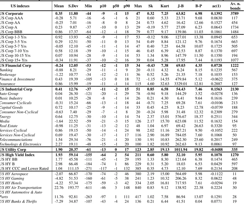
3. Descriptive statistics on the dependent variable

Descriptive statistics for a synthesis of our fixed bond indexes are reported in

Table A1 in the Appendix. Indexes are ranked by rating, maturity and industry

classifications, the latter available for both IG and HY bonds only for US.

4

_{Bonds with residual maturity below one year are excluded by Merrill Lynch from the universe of}

assets considered when building the indexes.

5

_{Corporate bond markets are far more illiquid than government bond markets. Transaction costs on}

the former may reach 1 or 2 percent of nominal value against .10-.15 on the latter.

6

_{We select for descriptive analysis 87 out of 207, 36 of 125 and 35 out of 118 indexes for US, UK}

and Eurozone markets respectively. Extended descriptive results for rating group/maturity and the

industry/maturity classifications are available upon request.

These statistics show that OAS volatility is monotonically increasing in credit

risk, while it is quite stable along the maturity curve. The maximum change of the

total US IG index is of 45 bps, while it is smaller, and around 20/30 bps, for the UK

and the Eurozone. IG industries with the highest delta credit spread volatilities are

Auto and Telecommunications in the United States, Capital Goods and Telecom in

the UK and Technology & Electronics in the Euro area.

As expected, HY indexes have much higher volatility than IG indexes (the HY

B-rating index volatility is twelve times higher than that of the AAA index in the US)

with a maximum of monthly changes for the aggregate HY index of 211 bps. The

Euro area total HY index is more volatile than both UK and US ones. When we move

from the next to last (B) to the last (CCC-C) rating group, volatility almost doubles in

the US and UK and gets three times higher in the Euro area. Air Transportation,

Insurance and Telecom are the highest volatility HY indexes in the US (up to a

maximum monthly change of more than 1200 bps).

The presence of the first two

sectors among those with highest volatility may be clearly related to the effects of the

terrorist attack of September 11 on financial markets.

Skewness, kurtosis and Jarque-Bera tests show that our OAS series are

nonnormal and have excess kurtosis exactly as stock return series. First order

autocorrelation coefficients and Box-Pierce diagnostics reveal the presence of a

certain degree of autocorrelation in these series.

4. The determinants of option adjusted credit spreads

4. 1 Interest rate variables

Interest rate changes are considered among the main determinants of credit spreads.

Empirical literature on term structure stochastic models identifies two

components explaining most of the time variability of risk free returns.

Ex-post,

these components are highly correlated (in decreasing order) with the level of interest

rate and the slope of the yield curve. These variables are then natural candidates for

being included as regressors in empirical estimates.

The level is generally represented by the return of a 10 or 5-year benchmark or

of a government bond index. The slope of the yield curve may be represented by the

spread between two different maturities or two representative indexes including all

bonds between two different maturities (i.e. IG 1-3 and IG 7-10). We will follow both

7

_{HY Merrill Lynch indexes do have an industry breakdown in the US, but not in the UK and}

Eurozone, due to the different development of HY bonds in the three financial markets. Just

consider that in the US the HY index includes on average 1270 bonds against 31 and 94 in the UK

and in the Eurozone area respectively. Data on US yield sectors are reported in Table A2 in the

Appendix.

approaches. Individual government bond data are from Bloomberg, while those on

government indexes from J.P.Morgan.

Some models include return volatility as an additional explanatory variable to

levels or yield curve slopes (see, among others, Longstaff and Schwartz, 1995). We

follow this path by using Bloomberg monthly data on the implicit volatility of options

on bond futures, where the underlying asset of these futures is represented by bonds

at the most significant maturities (such as 5, 10 or 30 years in the US, UK, and

Germany).

As it is well known, implicit volatility is forward looking and expresses

better than historical volatility current investors’ expectations on the volatility itself.

Despite it, since options on bond futures are mainly developed in the US, we collect

also historical volatility to compare results on different markets. Historical volatility

refers to benchmark government bonds from Bloomberg and J. P. Morgan data. Our

variable is the monthly change of the monthly historical and implied volatility

calculated on daily prices.

We measure from J.P.Morgan data the implicit volatility of OTC

(over-the-counter) options such as swap options, which represent the most liquid and widely

used hedging instrument in the bond market. The swap rate is a “refreshed AA credit

quality rate”

_{, and therefore is a benchmark rate for the corporate market and its}

volatility should be fundamental for bond valuation.

Finally, we build with J.P.Morgan data the skewness of options on bond futures,

given by the difference in the implicit volatility between “deep out-of-the-money”

(deep OTM) and “at-the-money”

(ATM) options. The skewness (or skew) is a

measure of market expectations on the degree of risk of significant and large future

changes in interest rates. This is because the difference between the implicit volatility

(and, consequently, the cost) of OTM with respect to that of ATM options gets larger

when expectations on larger interest rate movements are formed in the market. An

increase in the “skew” implies higher costs of contingent hedging against significant

interest rate changes. We compute the variable by using implicit volatility for OTM

options on bond futures with one, two, three and four strikes out-of-the-money

. The

skew is the difference in basis points between OTM and ATM options.

A final variable considered in the analysis is the implicit volatility of options at

long maturities (or vega). The normal maturity for options on interest rates (one up to

9

_{The 10-year Bund is the reference future in the Euro area.}

10

_{The credit risk difference between an AA corporate bond and a generic swap rate (which is an}

AA by definition, being based on the Libor rate) depends on the fact that the latter has no

downgrade risk, since we assume that the rating is constant in any resetting. The parallel with a

corporate index is clear: corporate indexes, when defined according to the rating grade, have a

“refreshed credit quality”. Consider though that an individual bond rating may vary before

rebalancing given that the bond will be excluded from the index only at the end of the month.

_{In swaptions “moneyness” is clearly evaluated on swap forward rates. Hence, an at-the-money}

option is an option defined on the at-the-money forward rate with maturity equal to the option

maturity.

12

_{The change in basis points is different according to the future and the underlying bond maturity.}

The change in basis points for a point (or strike) change will be larger for a bond with longer

duration.

six months) implies a higher influence of the underlying asset on the option value.

With maturities from 5 up to 15 years, exchanged in the swaptions market, changes in

the value of the underlying asset have a relatively lower impact while much higher is

the effect of changes in absolute volatility. This kind of options is in fact mainly used

to hedge on future expected interest rate volatility. Our variable is the J.P.Morgan

implicit volatility of swaptions on 5-year forward interest rates with 5-year maturity

(5-year 5-year forward), and on 15-year forward interest rates with 15-year maturity

(15-year 15-year forward).

4.2 Stock market variables

The effect of stock market variables on credit spreads is predicted by structural

models (Merton, 1974) which illustrate how positive stock returns increase the value

of firm asset and reduce the probability of failure. The same structural models predict

the

positive effect of firm asset volatility on credit spread.

We proxy this variable with historical volatility of stock market indexes and

with implicit volatility of options on the main stock market indexes. Moreover, we

also include among potential regressors the skew of implicit volatilities (the

difference between implicit volatilities of OTM and ATM put options). The rationale

is that an increase in this specific skew measure implies an increase in the perception

of risk generated by large negative movements of stock prices (Collin-Dufresne,

Goldstein, Martin, 2001). Given that a corporate bond is equivalent to a risk free

bond minus the value of a put option on firm asset (Merton, 1974), the skew is

expected to be positively correlated with credit spreads

_{. We calculate the skew as:}

(

) (

)

skew

=

σ

strike

−

σ

ATM

where

σ

is the implicit volatility and the OTM option

strike is 20 percent below the ATM option strike. We calculate the skew for the most

liquid maturities and try alternatively the one month and three month ones. As

additional relevant stock market variable we include the orthogonal risk factor SMB

built by Fama and French (1995)

as a proxy of specific small size risk. Given that this

variable is constructed as a differential in stock performance of small vs large firms,

it can therefore be linked to a spread reduction in corporate bonds (and so, to a

positive return), in the same manner as the SMB factor in the Fama-French approach

is connected to an increase in stock returns

_.

13

_{Since the put option is on the index and not on the individual stock, the observed empirical}

relationship may be weaker than the theoretical one. The same reasoning goes for stock index

returns or for its implied volatility. Listed options are always defined on more liquid and

representative large capitalisation indexes (such as the Standard & Poor’s 100), while corporate

bond indexes have generally higher coverage of the universe of bonds traded in the market. This is

another factor which inevitably weakens the links between theoretical framework and empirical

analysis.

14

_{In a parallel way, we also constructed the HML factor of Fama and French (1995), based on}

market to book ratio. Both SMB and HML factors are constructed with the relevant stock market

index constituents, different for the three areas.

4.3 Macroeconomic indicators

Since credit spreads measure excess risk of corporate with respect to

government bonds they are obviously expected to be negatively correlated with the

business cycle (see, among others, Van Horne, 2001; Duffie and Singleton, 2003).

To evaluate this effect we use Conference Board leading, coincident and lagging

indicators. The leading indicator is the weighted average of 10 indexes;

the

coincident indicator is an average of 4 indexes

and measures the current state of the

economy, while the lagging indicator is an average of 7 indexes.

Even though these

indicators have some of the components included in our estimates as individual

variables, they are weakly correlated with such components and have a different

meaning. We therefore include them in our analysis.

For the UK area we use leading and coincident Conference Board indicators. As

in the US these indicators are averages of (respectively 9 and 4) individual

components.

For the Euro area we use the Handesblatt leading indicator,

the”Economic

Sentiment Indicator” (ESI) and the “business climate indicator” of the European

Commission

_.

4.4 Default rates and transition matrices

Default rates and information on downgrades/upgrades operated by rating

agencies are another group of variables which may significantly affect OASs. From a

theoretical point of view, the event of bankrupcty of a given firm may affect credit

spread indexes, if the event is not anticipated by the market and is interpreted as a

signal of a worsening of aggregate credit risk. In this perspective failures of a

company in a given industry should affect more credit spread indexes of the same

15

_{The “leading” indicator is a weighted average of: Average Work Week, Jobless Claims,}

Consumer Orders, Stock Prices, Vendor Performance, Capital Orders, Building Permits, Consumer

Expectations, Money Supply, Interest Rates.

16

_{The “coincident” indicator is a weighted average of: Nonfarm Payroll, Personal Income,}

Industrial Production, Trade Sales.

17

_{The “lagging” indicator is a weighted average of: Average Duration, Inventory/Sales ratio, Labor}

Cost per Unit ratio, Prime Rate, Loans, Credit/Income ratio, CPI of Services.

18

_{The same approach is followed by Huang and Kong (2003).}

19

_{The UK “leading” indicator is a weighted average of: Order Book, Output Volume, Consumer}

Confidence, House Starts, Interest Index, FTSE Index, New Orders, Productivity, Corporate Op.

Surplus. The UK “coincident” indicator is a weighted average of: Employment Index, Industrial

Production, Retail Sales, Household Disposable Income.

20

_{The leading indicator is built using Handesblatt information and is a weighted average of:}

Industrial Confidence, Consumer Confidence, Industrial Production, Monetary Aggregates,

Harmonized Inflation, Curve.

21

_{The Economic Sentiment Indicator is a weighted average of: Industrial Confidence, Consumer}

Confidence, Construction Confidence, Retail Trade Confidence. The Service Confidence, an

indicator as well of the European Commission, is not part of the ESI.

industry and a downgrade of a large representative firm may have stronger impact

than that of small firms. Default rates and downgrades are generally anticyclical (see,

among others, Duffie and Singleton, 2003).

To test the effect of these variables we use Moody’s default rates, divided for IG

and HY in the US, UK and Europe rating transition matrices

_{for different areas, on}

a monthly basis. Default rates represent the share of firms (IG or HY in the US, UK

or Eurozone) who went default among those observed by Moody’s. Transition

matrices indicate the frequencies of firms falling into different rating classes in a

given period, given the rating class of the beginning of the period.

We exploit the unique advantage of having these data on a monthly basis to

build a monthly downgrade ratio calculated as:

down

downgrades

all

=

where

the denominator is represented by the relevant group of corporations observed by

Moody’s in a given geographical area or aggregate asset class. We therefore have

three indicators for any areas (IG, HY and total).

4.6 Liquidity variables

Liquidity effects are expected to be highly relevant on credit risk changes in a

typically illiquid OTC market such as that of corporate bonds (Driessen, 2002).

Bid-offer spreads would represent the exact measure of transaction costs, but this variable

is not available, not only for academic research, but also in investment banks

databases, such as those of Lehman Brothers and Merrill Lynch, which

conventionally quote bond bid prices in their indexes.

A typical proxy which can be used is government bond bid-offer spreads, and,

possibly, those of the more illiquid non – benchmark government bonds.

Furthermore, it is well known that, in presence of an increased perception of

market risk, “flight-to-quality” effects may increase

the spread between benchmark

or “on-the-run” and “off-the-run” (or ex benchmark) government bonds.

. We

therefore build series of these spreads for the US, the UK and Germany

on 10 to 30

year maturities.

Another liquidity indicator, typically considered in the literature, is the swap

spread, or the spread between government bond and the swap rate; the assumption is

that a reduced liquidity in the swap market necessarily implies a parallel and

22

_{This matrix is generally called transition probability matrix. Strictu sensu the definition is not}

correct since we have historical transition frequences and not ex ante transition probabilities.

23

_{Benchmark ( “on-the-run”) bonds typically have a longer time to maturity and, consequently, a}

higher theoretical yield to maturity than “off-the-run” bonds. With flight to quality the yield curve

may invert (in that point), with a liquidity premium which justifies, for the “on-the-run” bond, a

yield to maturity lower than that of the “off-the-run” bond.

24

_{As already mentioned before, German bonds are generally taken as a reference from investors for}

the Euro area.

25

_{Consider that liquidity and change in the perception of risk may coincide, as higher perception of}

risk generates flight to quality effects which induce investors to move from less liquid to more

liquid bonds.

amplified effect in the corporate bond market (Collin et al. 2001). In reality, the swap

market has become increasingly more liquid so that changes in the swap spread are

unlikely to measure significant liquidity effects. Moreover, the swap spread is a

measure of the excess return of a generic AA financial corporate bond over the

government bond. This is because it is built on the Libor rate, which is generally

applied to an AA grade (banking sector) issuer. Since the index is reset every half

year or every year, it can be viewed as a “refreshed credit quality” yield, and

therefore as intrinsically less risky than an AA corporate bond which may suffer from

a deterioration of credit quality in time. Hence, the swap spread is a downward biased

proxy of the risk differential between a high grade corporate bond and a government

bond. To analyse this effect we collect from Bloomberg swap spread monthly

changes in basis points for 5, 10 and 30 year maturities in the US, UK, and in the

Euro area.

4.7 The role of institutional investors

The last proxy of liquidity considered is represented by buy and sell flows on

corporate bonds recorded by Lehman Brothers from 1998. These data measure

quantities (in billions of dollars) on monthly basis of purchases and sales made by

institutional investors with Lehman Brothers. Even though the variable refers only to

the US market, and only to volumes intermediated by Lehman Brothers as market

maker, it represents a significant share of total volumes given the investment bank’s

leadership in the fixed income market.

We introduce this variable to test whether institutional investors with their

sales/purchases signal to the market additional information, not incorporated in other

regressors such as stock performance or in business cycle indicators; in particular, an

increase in purchases (sells) could be a signal of reduced (increased) perception of

risk, and therefore have negative (positive) impact on the spreads.

5.1 Empirical findings on separate estimates

In the previous section we provided rationales for the inclusion of all the

variables described in the estimates. The number of these variables, though, is too

high and some of them proxy for the same underlying factors. Hence, the joint

inclusion of all of them in the estimates may create serious problems of

multicollinearity. We therefore decide to divide the empirical analysis in two steps.

In order to evaluate the significance of different variables we perform separate

estimates for each subgroup of variables as a first step using as a dependent variable

corporate bond indexes of different subgroups classified by rating, maturity and

industry. In Table 1B we report synthetically the number of times (in percent) the

variable is significant in these estimates. In a second step we perform an estimate

with a selected group of indicators which have been shown to be significant at least

20 percent of times in the separate estimates. We select as regressors: among interest

rate variables, the 5 year yield and the spread between US and UK (or Euro) bond

yields

_{; among stock market variables, the return on the relevant index, the implied}

volatility on the index, and the SMB factor

_{; among the business cycle indicators,}

the US leading indicator

; among the liquidity indicators, the swap spread

. We also

use for US estimates the institutional investors data

.

We finally check the robustness of our results repeating the estimates for

different subsample splits, performing structural break tests, and with higher (weekly)

data frequency.

Given the autocorrelation and nonnormality of OAS evidenced by descriptive

statistics presented in the Appendix we use heteroskedasticity and autocorrelation

robust Newey-West (1987) standard errors. The optimal selection of the truncation

lag is achieved by following the automatic selection approach followed by Newey

and West (1994).

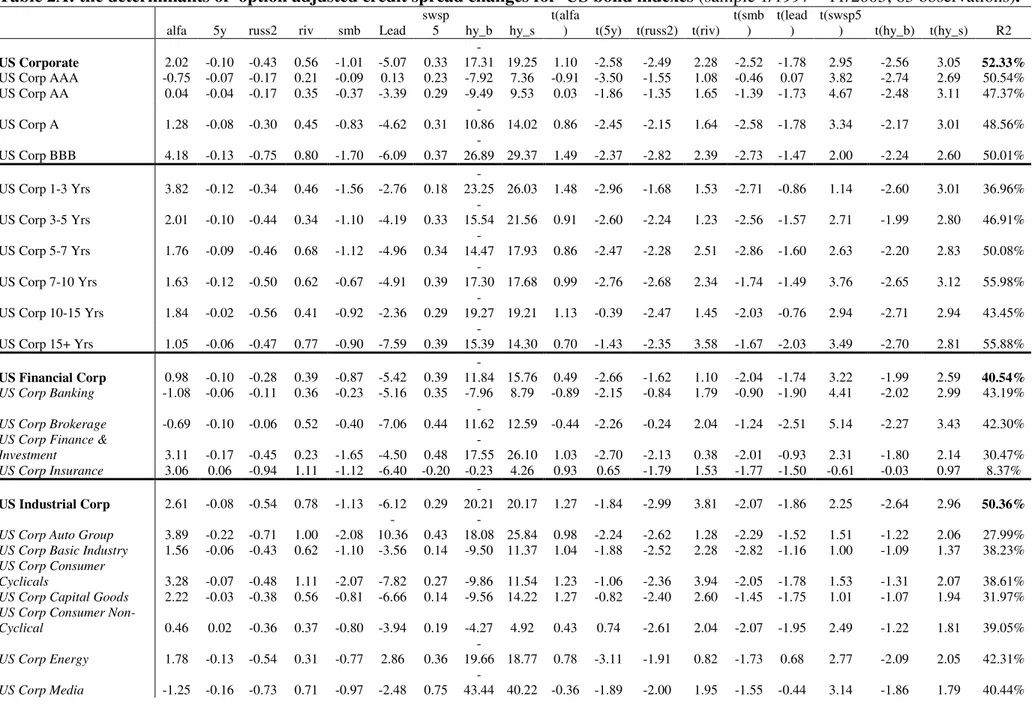
5.2 Empirical findings on the final selected specification for the US area

In this section we outline an empirical specification in which a selected number

of the described regressors is included. Following Huang and Kong (2003), we select

them from a larger set to perform a parsimonious estimate.

The chosen specification for US delta credit spread is the following:

( )

(

)

( )

(

)

(

)

(

)

(

)

(

)

5

2

5

_

_

t

t

t

t

t

t

t

t

DCS

y

russ

riv

smb

lead

swsp

hy b

hy s

α β

β

β

β

β

β

β

β

ε

= + ∆

+

+ ∆

∆

∆

∆

∆

+

+

+

+

+

+

+

(1.1)

where DCS (Delta Credit Spread) is the change of the option adjusted credit spread,

5y is the 5-year Treasury bond yield, russ2 is the return of the Russel 2000, riv is the

implicit volatility of the options on the Russell 2000,

_{smb is the Fama-French}

27

_{We find equivalent results using J.P. Morgan bond index returns and bond yield variation, and we}

therefore choose to use the latter. Moreover, we find yield curve, and both implied (including skew

and vega) and historical yield volatility not very powerful in explaining credit spread changes.

_{We instead exclude HML factor and skew.}

29

_{The US Leading Indicator proves to be much more reliable even for UK and the Euro area,}

respect to “local” indicators, showing the linkage of credit spreads to the US economy.

30

_{The spread between on-the-run and off-the-run government bonds is significant in UK and in the}

Euro area, but not in the US; given it has a very small coefficient, however, we exclude it from the

regressor set. We also exclude bid-ask spread variations.

31

_{We exclude instead the downgrade and the default ratios. They are significant only in the Euro}

area, but from inspection of the data this result comes from a unique default not expected in the

market (Ahold, October 2002). This result confirns the fact that credit spreads on average are

sensitive only to unexpected and relevant credit events.

32

_{Even if treasury bonds returns have been shown in the previous empirical literature not to be}

strongly correlated with volatility, credit spreads could nonetheless be affected by volatility, and not

only of the assets, as suggested by Merton’s work (i.e. equity volatility for empirical reasons), but

also of the underlying risk free interest rates (bonds volatility). In fact, investors could demand a

Small-minus-Big factor, lead is the Leading Indicator del Conference Board, swsp5 is

the spread between swap and yield of 5-year government bond, hy_b (hy_s) are total

HY US bond purchases (sales) of Lehman Brothers professional investors.

Our results, presented in Table 2A, show that this set of regressors explains a

significant part of credit spread variability. The adjusted

_R

_{ranges from 52.33% for}

the overall IG index to the 56.89% for the HY index. The index with the highest

R

is the 5-7 year High Yield (61.67%). All of the selected variables maintain significant

explanatory power when jointly considered. The change in the interest rate level (5y)

is statistically significant for almost all indexes. An increase in the yield of the 5-year

Treasury bond of 10 basis points generates a reduction of the spreads of 1 bp (8 bps)

for the aggregate Investment Grade (High Yield) index, consistently with our

previous estimates in which only interest rate variables were included.

Telecommunications and Auto are the industry indexes that are more sensitive to this

variable.

Stock returns (russ2) are statistically significant along the rating curve, with the

exception of the AAA and AA corporates. This result confirms that riskier bonds are

more dependent from stock returns. For a 10% positive return of the Russell 2000, we

observe a reduction of the spreads ranging from 3 bps for the A rating index to 24 bps

for the B rating, up to 42 for the CCC-C rating index. Among macroindustries the

coefficient is the highest for industrials, and, among single industries, for cyclical

industries such as Auto, Telecom and Tech industries. As expected, coefficient

magnitude is higher for Consumer Cyclicals and Services Cyclicals with respect to

the corresponding non cyclicals (Consumer Non-Cyclicals, Services Non-Cyclicals).

Stock market implicit volatility (riv) has a stronger impact on riskier bond

indexes, confirming their relatively higher dependence from expectations on stock

market variability. T-stats are significant for BBB and CCC-C indexes. Coefficient

magnitudes show that a one percent increase of the implicit volatility widens spreads

of almost one basis point for the BBB index and up to 6 bps for the CCC-C index.

The most sensitive macroindustry (industry) is Industrials (Telecom). The High Yield

telecom bond index exhibits

the highest reaction to the same one percent change of

the implicit volatility, with an increase in the spread of almost 10 bps. The

Small-minus-Big risk factor has significant effects, which are increasing along the rating

curve, up to a maximum of a 10 bps reduction of the credit spread for a one percent

variation of the regressor. The variable is significant also for industry specific

indexes, with the exception of Banking and Telecommunication.

premium in the markets to hold a corporate bond, that is mainly valued on a spread basis, if the

underlying risk free rate is more volatile.

33

_{We also add in a robustness check lagged values of the regressors in our specification and find}

that results are robust to their inclusion, being not statistically significant. This could also be

justified by the fact that data have monthly frequency, and markets tend to react quickly to new

information.

34

_{Results for US high yield sectors are reported in Table A2 in the Appendix.}

35

_{An interpretation of this result is that these two indexes are composed by larger companies and}

therefore are less subject to small size risk.

The Conference Board Leading Indicator (lead) becomes weakly significant in

presence of all other regressors. We must consider, though, that it is a composite

indicator of different variables, some of them present in the estimates. As expected,

its impact is higher on cyclical than on non cyclical industries, as it is possible to

observe directly in the comparison between its effect on Consumer Cyclicals (78

bps) and Consumer Non-Cyclicals (39 bps).

The change of swap spreads (swsp5) is statistically significant with an effect

which is inversely related to the rating curve. A 10 bps increase of swap spreads

generates an increase in the dependent variable ranging from 2 bps of the AAA index,

to 8 bps of the BB, up to 26 bps of the CCC-C index. The impact of a change of the

same magnitude in the regressor is quite stable across IG industries, with a widening

of the credit spread of around 3-4 bps on Financials, Industrials and Utilities.

Regressors measuring purchases and sales of High Yield bonds from

institutional investors are highly significant. A flow of 100 million dollar

purchase

(sale), generates a reduction (increase) of credit spreads of around 2 bps on the

aggregate IG index. Telecommunications is the most sensitive industry with an effect

of around 5 bps. This result confirms that institutional investors trades signal to the

market information not already captured by other controls included in the estimates

(expectations on future volatility, stock market performance including expectations

on future earnings, etc.).

5.3 Empirical findings on the final selected specification for the UK area

For the UK area we choose the following specification:

( )

(

)

(

)

(

)

(

)

(

)

(

)

5

5

_

_

_

10

DCS

y

sp y

ftse all

ftse iv

smb

lead us

swsp

α β

β

β

β

β

β

β

ε

= + ∆

+ ∆

+

∆

∆

∆

+

+

+

+

+

+

(1.2)

where 5y is the 5-year UK Treasury yield, sp_5y is the spread between the 5-year US

and UK government bond, ftse_all is the return of the Ftse All Share index, ftse_iv is

the implicit volatility of options on the Ftse 100, smb is the Fama-French

Small-minus-Big factor, lead_us is the Leading Indicator of the US Conference Board,

swsp10 is the spread between the swap rate and the 10-year government bond yield

.

Our results, presented in Table 2B, show that goodness of fit is lower than in the

US estimate.

_R

_{are around 40% and 44%, respectively, for the aggregate Investment}

Grade and High Yield indexes. The highest R

is 49% for the IG 5-7 year index.

Differently from the US specification, not all the selected variables, which were

highly significant in the specific estimates, maintain their significance when jointly

included in the regression. Interest rate variables, such as the 5-year level and the

spread with the US Treasury bond, are sheldom significant. The Footsie stock return

is significant for the aggregate HY index, but not for the aggregate IG index

. In the

36

_{Data on buy or sell flows (Table 2A) are measured in billions of dollars.}

_{The 10-year replaces the 5-year swap spread in the UK area for lack of data.}

38

_{The CCC-C index makes an exception with non significant regressors (except for the Leading}

Indicator) and a very low R-square. Consider though that the index is made of only 4 bonds on

first case a 10% positive stock return generates a reduction of the High Yield credit

spread of 60 bps. The implicit volatility is also not significant, with the exception of

the HY BB index, where an increase of 1 percent in the variable generates a 2.5 bps

increase in the spreads. The SMB factor is strongly significant for some indexes and

weakly significant for others. The stronger impact is on the B index, where an

increase of 1 percent in the variable generates a 6.5 bps increase in the spreads. The

US Leading indicator, a proxy of the impact of US business cycle on the UK market,

has strong impact on Industrials, and, within industrials, on Capital Goods, where a

change of one point in the indicator generates a reduction of the OAS of 8 bps. Its

impact is also decreasing in the quality of credit rating. Changes in the swap spreads

are significant for IG indexes, but not for HY indexes. Their impact is quite stable

across different ratings and macroindustries (.5 bp increase in the spread for a

positive change of 1 bp).

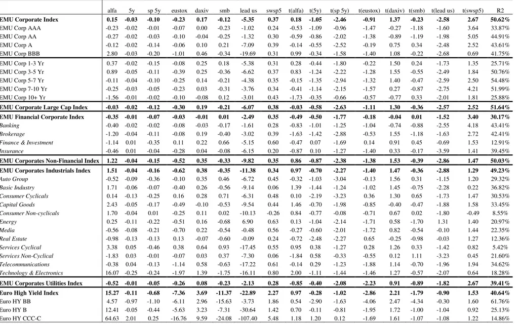
5.4 Empirical findings on the final selected specification for the Euro area

For the Euro area we choose the following specification:

( )

(

)

(

)

(

)

(

)

(

)

(

)

5

5

_

_

5

DCS

y

sp y

eustox

dax iv

smb

lead us

swsp

α β

β

β

β

β

β

β

ε

= + ∆

+ ∆

+

∆

∆

∆

+

+

+

+

+

+

(1.3)

where 5y is the yield on the 5-year German government bond, sp_5y the spread

between the 5-year US and German government bond, eustox is the return of the

Eurostoxx index, dax_iv is the implicit volatility of the options on Dax, smb is the

Fama-French Small-minus-Big factor, lead_us is the Leading Indicator of the US

Conference Board, swsp5 is the spread between the swap rate and the 5-year German

government bond yield.

Empirical findings are reported on Table 2C.

R

varies according to the

selected dependent variable ranging from 50.62% for the aggregate IG index, to

40.64% for the aggregate HY and reaching its peak (61.76%) for the HY BB index.

The change of government indexes is significant only in a few cases, while the spread

with US Treasury bonds has higher explanatory power for IG indexes. Its highest

impact is on Industrials where a rise of the US-German spread of 10 bps generates a

1.5 bps increase in credit spreads of. Among individual industries, the most sensitive

to this variable are cyclical ones such as Auto, Consumer Cyclicals, Services

Cyclicals. Stock market variables are significant for HY, but not for IG indexes. A

10% positive stock return of the Eurostoxx index generates a credit spread reduction

of around 6 bps for the BB index and of 16 bps for the CCC-C index. An increase of

one percent in the implicit volatility on Dax (daxiv) generates a widening of credit

spreads of 3 bps for the BB index and of around 10 bps for the CCC-C index. On the

other hand, a positive one percent change of the Small-minus-Big factor generates a

reduction of credit spreads of the HY index of around 11 bps. The US Conference

average and is therefore highly illiquid and hardly representative. As a comparison, the

corresponding US index is made by 208 bonds.

Board Leading Indicator (lead us) has significant effects on Investment Grade

indexes. The effect of an increase of one point in the indicator is decreasing in the

quality of credit rating, ranging from 1 bp for the AAA to around 20 bps for the BBB.

The impact on macroindustries is higher on Industrials (around 10 bps) and, as

expected, lower on Financials (2.5 bps) and Utilities (2 bps). Telecommunications

and Technology & Electronics are the industries which are most sensitive to this

variable (respectively 17 and 16 bps). The swap spread is significant for IG corporate

indexes up to the A rating. The impact is almost constant along the yield and rating

curve, and across macroindustries.

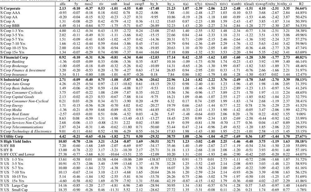
5.5 Comparisons of our findings across the three markets and with the recent

literature

For a more direct comparison of results across macroareas we restimate the

model (Tables 3A-3B) for the same time interval starting from January 1999 which is

the first date in which information on Eurozone markets is available. Limits in this

comparison are that indexes in different macroareas have not the same degree of

representativeness

_{and regressors are obviously not exactly correspondent with each}

other (i.e. stock indexes may have different scope and coverage).

A comparative inspection of estimates shows that goodness of fit is higher in the

US than in the UK area. The result may be affected by the difference in

representativeness between the two indexes.

The effect of a change in the level of interest rates (and spread against US for

UK and Eurozone area) of 10 bps generates a change in credit spreads of around 1 bp

for IG indexes, and around 7 and 8 bps for High Yield US and Eurozone indexes.

The effect is not statistically significant in the UK area. An interesting and

comparable result is the effects of stock returns. A ten percent change in the stock

index is significant on IG indexes only in the US, where it generates a reduction of

the spreads of around 4 bps

. The interesting point is that the effect of stock returns

on HY indexes is significant in any of the three areas but the magnitude is widely

diversified (22 bps in the US, 45 bps in the UK and 73 bps in the Eurozone area). It

would be interesting to investigate (if we can exclude or minimise the effect of

differences in the dependent variable and regressors in the three markets) whether

this difference may be attributed to different risk attitudes of investors or to

regulatory differences affecting the capacity of firm recovery (and/or creditor rights)

under financial distress in the three different areas (i. e. Chapter 11 vs bankruptcy

laws in the UK and Europe). We argue that this finding cannot be solely explained in

terms of heterogeneity in variables measured across different markets since the

comparisons of other effects such as that of implicit volatility on stock index options

39

_{Index representativeness is highly heterogeneous across different markets. The IG index includes}

3789, 1159 and 478 bonds respectively in the US, Eurozone and UK area. The equivalent numbers

for the HY index are 1270, 94 and 31.

40

_{UK and Eurozone estimates have coefficients of the same magnitude but t-stats are not}

significant.

on HY indexes are substantially equivalent in the three areas. A one percent increase

in the implicit volatility enlarges BB indexes credit spreads of 2.7, 2.5 and 3 basis

points in the US, UK and Eurozone areas respectively.

_{However, the one percent}

change in the SMB factor reduces the BBB index credit spread of 1.7 bps in the US,

and 1.3 in the UK

_{. The effect of the US Leading Indicator (the same variable for all}

markets) is also comparable in all areas generating a reduction of credit spreads with

an increasing effect along the credit curve of IG indexes confirming the sensitivity of

UK and Eurozone financial markets to the US business cycle. Swap spreads (on the

5-year maturity for the US and Eurozone, and on the 10-year maturity for the UK

)

have a comparable effect in the three areas. A 10 bps increase in the swap spread

generates a widening of credit spreads of around 4 bps in the three markets.

To sum up, the analysis outlines common determinants of credit spread changes

between US and Euro zone. Regarding interest rates, european long term yields tend

to covariate with US bonds; using the spread between the two areas as a regressor, we

insulated the effect in the analysis. Even if ECB did not change rates in this period,

interest rate term structure is a function, between other things, of expected growth

and inflation, and US cycle seems to have a great impact on the Euro zone. This is

confirmed, on the other hand, by the results regarding US leading indicators, which

are shown to exhert an important influence on european credit spreads.

6. Robustness check

We perform two robustness checks on our results: i) Chow tests to control for

structural breaks, and ii) reestimation of the model with higher frequency data.

We first divide the sample in each of the three areas into two subperiods

_and

perform a Chow test to check for structural stability of the model.

_{The absence of}

structural breaks is rejected at the five percent significance level for 6 indexes in the

US estimates

, (US Corp AAA 15+ Yrs, U.S Industrial Corp AAA, US HY

Containers, US HY Restaurants, US HY Textiles/Apparel, HY US B 10+ Yrs) for

one index in the Eurozone estimates (European Currency High Yield BB Rated) and

for no indexes in the UK estimates.

Given the high number of indexes considered

_{the number of cases in which the}

null is rejected is extremely low: less than 3% in the US, 1% for the Eurozone area

41

_{Implicit volatility is significant also for IG US indexes, where a one percent increase widens}

spreads of 0.5 bps.

42

_{It is significant for the HY Eurozone index with a coefficient of 11 bps.}

_{The 10-year replaces the 5-year swap spread in the UK area for lack of data.}

44

_{Subperiod estimates are omitted for reasons of space and are available from the authors upon}

request.

45

_{We use sample halves as breakpoints in each geographical market. Consequently, the last month}

of the first subsample is May 2000 for the US, November 2000 for the UK and June 2000 for the

Eurozone.

46

_{Huang and Kong (2003) reject the null of no structural break for two (AA-AAA 15+ Yrs) out of}

nine considered indexes.

and nil for the UK. This result emphasizes the substantial stability of parameters in

our estimates.

We perform the second robustness chek by repeating our estimate on higher

frequency series (weekly instead of monthly data). We calculated weekly changes

using wednesday data in order to avoid end of week distortions generated by low

volumes or insufficient liquidity.

The choice of using higher frequency data has some costs. The first is that, in a

limited number of cases, the change is not measured by an index with the same

constituents. This is the case when two adjoining wednesdays belong to two different

months.

The other problem is the loss of all those regressors which cannot be measured

on weekly basis. We therefore cannot use the Conference Board indicator, the Fama

and French risk factor, and volumes of HY sales or purchases from institutional

investors. For this reason, we reintroduce in our estimates also other regressors which

we did not considered in our final estimates. These are the slope of the yield curve

and interest rate volatility. Furthermore, we do not have implicit volatility of options

on the Russell 2000, on the Bund future and on the Gilt. We replace them

respectively with the implicit volatility of the options on the Standard & Poor’s 100,

and with swap options on 10-year euro and sterling.

The final specification of the determinant of OAS on weekly basis on the US is:

( )

(

)

( )

(

)

(

)

(

)

5

2 _10

1

2

100

5

DCS

y

ty

russ

sp

iv

swsp

α β

β

β

β

β

β

ε

= + ∆

+ ∆

+ ∆

∆

∆

+

+

+

+

+

(1.4)

where 5y is the 5-year Treasury yield, 2_10 is the spread between 10 and 2-year

Treasury yield, ty1 is the implicit volatility (in basis points) of the options on the

10-year Treasury bond future, russ2 is the return of the Russell 2000, sp100iv is the

implicit volatility of the options on the Standard & Poor’s 100, swsp5 is the spread

between the swap rate and the 5-year government bond yield. Estimates results

(Table 4A) show that

_R

_{are smaller and some t-stat less significant (with respect to}

monthly frequency estimates) as expected given the loss of important regressors

and, presumably, the use of OAS changes across the end of month rebalancing of

indexes. Nonetheless, our

_R

_{s range from 24 percent of the total IG index, to 44}

percent of the total HY index. The highest value is 50 percent for the HY 5-7 Yrs

index. Interest rate levels, stock returns, swap spread, and implicit volatility on rates

for HY bonds are all significant and their coefficient are of magnitudes comparable

with those obtained in monthly estimates

, confirming robustness of our estimates to

changes in frequency.

48

_{When wednesday is an holiday we measure the change by using thursday data.}

49

_{These are sales and purchases of HY bonds from institutional investors, the Leading indicator and}

implicit volatility on Russel 2000, which was shown to be more significant than S&P100 implicit

volatility in monthly estimantes.

50

_{As an example estimates of the impact on the overall IG US index of interest rate levels, stock}

return and swap spread exhibit coefficients respectively of -.10, -.43 and .33 in monthly estimates

and of -.10, -.32 and .29 in weekly estimates.

The specification of the determinant of OASs in the UK market on weekly data

is:

( )

(

)

(

)

(

)

(

)

(

)

(

)

5

5

2 _10

10

10

t

t

t

t

t

t

t

DCS

y

sp y

swo

ftsesm

ftseiv

swsp

α β

β

β

β

β

β

β

ε

= + ∆

+ ∆

+ ∆

∆

∆

∆

+

+

+

+

+

+

(1.5)

where 5y is the 5-year UK Treasury yield, sp_5y is the spread between the 5-year US

and UK government bond, 2_10 is the spread between 10 and 2-year UK Treasury

yield, swo10 is the implicit volatility of swap options on the 10-year rate, ftse_sm is

the return of the Ftse Small Cap index, ftse_iv is the implicit volatility of the options

on Ftse 100, swsp10 is the spread between the swap rate and the 10-year government

bond yield. Table 4B shows

_R

_{s ranging from 20% to 29% for, respectively, the}

overall IG and HY indexes. Interest rates, stock returns, implicit volatility and swap

spreads are statistically significant. Their coefficient magnitude is comparable with

that of monthly data, confirming the robustness of monthly data results.

The specification of the determinant of OASs in the Eurozone market on weekly

data is:

( )

(

)

(

)

(

)

(

)

(

)

(

)

5

5

2 _10

10

5

DCS

y

sp y

swo

eustox

daxiv

swsp

α β

β

β

β

β

β

β

ε

= + ∆

+

+ ∆

∆

∆

∆

+

+

+

+

+

+

(1.6)

where 5y is the 5-year Bund, sp_5y is the spread between the 5-year US and German

government bond, 2_10 is the 10-year- 2-year spread between German bonds, swo10

is the implicit volatility of swap options on the 10-year rate, eustox is the return of the

Eurostoxx index, daxiv is the implicit volatility of options on the Dax index, swsp5 is

the spread between the swap rate and the yield of the five year government bond.

Table 4C shows that our

R

2

s range from 0.41 of the IG index and 0.19 of the HY

index. Interest rate level and spread, stock returns, stock volatility and swap spread

are statistically significant and with coefficients which are comparable with those

from our monthly estimates.

The analysis on the three markets commented in this section seems to show that

significance of determinants of delta credit spreads is quite robust to changes in data

frequency and sample period.

7. Conclusions

We analyse the determinants of the variation of option adjusted credit spreads

(OASs) on a unique database which enlarges the scope of the analysis of the current

empirical literature to more disaggregated indexes (combining industry, grade and

maturity levels), new variables (volumes of sales and purchases of institutional

investors; monthly downgrades and default frequencies) and additional markets (UK

and the Eurozone). Our results explain a higher portion of credit spread variability

(adjusted R squared up to 61 percent for the US, 49 percent for the UK and 61

percent for the Euro area) than recent literature empirical findings which focus on the

US market only.

The variables which are more significant are the same across the three markets

(changes in interest rates, changes in the swap spread, stock market returns, implicit

volatility of stock index options, leading indicators of the business cycle and

purchases and sales of HY from institutional investors for the US market). The

significance of a variable which has never been considered in the literature

(purchases and sales of HY from institutional investors) seems to confirm that trading

decisions of institutional investors bring into the market information which is not

captured into stock market performance, implicit volatility and other regressors

considered in the estimates.

Our results confirm that HY indexes and cyclical industries (such as

Automotive, Consumer Cyclicals, Services Cyclicals, e high tech) are much more

sensitive to stock market and business cycle variables than, respectively, IG indexes

and industry non cyclical indexes.

Comparability across different markets shows that DCSs determinants have

effects which are quite similar in magnitude in the three areas, in spite of the

inevitable heterogeneity in regressors and in representativeness of bond indexes. A

relevant exception is the largely higher significance of stock returns on HY bonds in

the Eurozone than in the US area. We suggest that differences in bankruptcy

regulation across different markets may affect this result. Another relevant

cross-market result is the effect of US leading indicator on UK and Eurozone OAS, and the

spread between US Treasury and Gilt or Bund, confirming the sensitiveness of the

two European markets to the US business cycle.

Finally, the lack of significance of Moody’s monthly default rates

_{suggest that}

these data do not add on average significant information to that already incorporated

in the credit spreads.

51

_{Collin-Dufresne, Goldstein, Martin (2001) explain between 20% and 30% of credit spread}

variabilitty of US industrial bonds between July 1988 and December 1997, and up to 40% when

they use lagged variables in levels. Elton, Gruber, Agrawal, Mann (2001) explain up to 30 percent

of the spread unexplained by default premium and tax distortions with a three factor Fama and

French (1995) model for Industrials bonds, concluding that large part of the risk is systematic,

exactly as in the stock market.