2
Alma Mater Studiorum – Università di Bologna
DOTTORATO DI RICERCA IN
Fisica Applicata
Ciclo _XXIVSettore Concorsuale di afferenza: __02/B3
Settore Scientifico disciplinare:____FIS/07
TITOLO TESI
Microscopic Modeling on Complex networks
Presentata da:
Pierandrea Petazzi
Coordinatore Dottorato
Relatore
Fabio Ortolani Sandro Rambaldi
_______________________
___________________
3
Index
Introduction ... 7
Microscopic Modeling Of Car Traffic ... 11
1.1 A brief history of traffic studies: state of the art, and how we got there ... 11
1.2. Some basic concepts and definitions ... 14
1.3 the Fundamental Diagram ... 15
1.4 Phase transitions ... 18
1.5. A brief review of car following models... 20
The Gazis-Herman-Rothery models (GHR). ... 21
Safety-distance or collision avoidance models (CA). ... 21
Linear models (Helly). ... 22
Psychophysical or Action Point (AP) models. ... 22
Fuzzy logic models. ... 23
1.6. What to do: a Physicist's standpoint ... 24
1.5 The model: Mobilis ... 25
1.5.1. The characteristics of roads in the Mobilis Model ... 27
1.5.2. Nodes in Mobilis ... 27
1.5.3. Car following dynamics ... 29
1.8. Analysis of some test networks ... 31
1.8.1. A single ring ... 31
1.8.2. Two interacting rings ... 36
1.8.3. A Manhattan-like road network ... 39
1.8.4. A Manhattan-like road network with roundabouts ... 43
1.8.5. A “chessboard” Manhattan Network. ... 45
2. Hysteresis phenomena and phase transitions in ideal urban mobility networks ... 47
2.1.The model and the fundamental diagram ... 47
2.2.The density distribution ... 49
2.3.Back on the macroscopic fundamental diagram, conjectures on phase transitions ... 52
Constant density ... 54
Constant inflow ... 56
2.4.Scale invariance ... 58
2.6.Introducing spatial inhomogeneity in the network ... 60
2.6.Tentative explanations ... 62
3.Road Hierarchy ... 65
4. Crowd Transplant ... 70
4
List of figures
Introduction ... 6
Microscopic Modeling Of Car Traffic ... 10
1.1 A brief history of traffic studies: state of the art, and how we got there ... 10
1.2. Some basic concepts and definitions ... 13
1.3 The Fundamental Diagram ... 14
1.4 Phase transitions ... 17
1.5. A brief review of car following models... 19
The Gazis-Herman-Rothery models (GHR). ... 20
Safety-distance or collision avoidance models (CA). ... 20
Linear models (Helly). ... 21
Psychophysical or Action Point (AP) models. ... 21
Fuzzy logic models. ... 22
1.6 What to do: a Physicist's standpoint ... 23
1.5 The model: Mobilis ... 24
1.5.1 The characteristics of roads in the Mobilis Model ... 26
1.5.2 Nodes in Mobilis ... 26
1.5.3 Car following dynamics ... 28
1.8 Analysis of some test networks ... 30
1.8.2 Two interacting rings ... 35
1.8.3. A Manhattan-like road network ... 38
1.8.4 A Manhattan-like road network with roundabouts ... 42
1.8.5 A “chessboard” Manhattan Network. ... 44
2. Hysteresis phenomena and phase transitions in ideal urban mobility networks ... 46
2.1.The model and the fundamental diagram ... 46
2.2The density distribution ... 48
2.3Back on the macroscopic fundamental diagram, conjectures on phase transitions ... 51
Constant density ... 53
Constant inflow ... 55
2.4. Scale dependencies ... 57
5
2.6. Tentative explanations ... 61
3.Road Hierarchy ... 64
4. Crowd Transplant ... 69
6
Introduction
The words of Philip W. Anderson in his article “More is different” are probably still today the best definition of complex system to be found: The constructionist
Hypothesis breaks down when confronted with the twin difficulties of scale and complexity. The behavior of large and complex aggregates of elementary particles it turns out is not to be understood in terms of a simple extrapolation of the properties of a few particles. Instead at each level of complexity entirely new properties appear, and the understanding of the new behaviors requires research which I think is as fundamental in its nature as any other(Anderson,
1972). In a nutshell, even the knowledge of all fundamental laws governing nature does in no way give us the ability to reconstruct and understand the universe, those properties that appear at new complexity levels are usually called emergent properties.
This definition unfortunately doesn’t provide us any useful tools to explore the vastness of the subject, but it gives us a connection between a whole plethora of phenomena that up to then was somehow ignored by the most quantitative sciences, and it allows to make analogies, which are all but new in physics, between emergent properties at very different scales, from elementary particles, to many-body physics, chemistry, molecular biology, physiology, up to entire organisms, societies, ecosystems.
A good idea of the topic comes up looking at an ants nest. A nest is a clearly visible macroscopic structure, a functionally efficient superorganism, its construction and management is performed by all the ants living in it, though no ant alone knows in detail the whole project, nor is aware of the structure, every ant just does its job, guided by instinct, and communicating with the rest of the ants mostly by the pheromones left by other ants. The whole nest is then
7
obviously something very different from a hypothetical sum of N ants. Looking at ants a little further there are more things to be discovered; there are “slaver ants” that steal eggs from other colonies to increase the workforce of their own, some of them can choose to do so, but there are species of ants which queen has no choice but attacking another colony, usurping the resident queen’s place, since they lack the ability to produce workers. There is also a beetle, the Lomechusa Strumosa, that acts somehow as a drug dealer to ants, being a social parasite of the colony, the beetle gives the ants some sugar-like psychoactive secretion, making the ants “lomecusomans”, inducing them to feed it rather than the queen and the larvae, and in the long term killing the queen and the whole colony. Another example is the Maculinea butterfly, when it is in caterpillar stage, if it falls from a tree, if found by myrmica ants, it tricks their sense of hearing and smell, mimicking the characteristics of one of their larvae. The ants take it back to the nest, and for a time variable from 11 to 23 months, the butterfly is a social parasite of the myrmica nest.
But even more surprising, there is some “second order” parasite of the maculinea, a wasp, the neotypus melanocephalus can in some still unclear way understand if there is a butterfly larva inside an ants nest in its cocoon phase, it then enters the nest, keeping ants at bay with some deceiving secretion that makes ants fight each other, and lays an egg inside the butterfly cocoon before it hatches.
A single organism or even just its nervous system is a complex system in its own right. Though most of the details in the way a brain works is still unclear, there is some overwhelming empirical evidence that it can reliably and effectively process information; a group of individuals can develop a language, a culture or a society and a set of laws governing it, that then evolves itself independently from any single member of the group, this goes further building
8
information giants such as the web 2.0 and its huge interconnected structure of social networks, blogs, individuals and circulating ideas, which can in turn show their effects in the real world and in real societies. Social networks changed the dynamics of more than a generation, and spawned whole new movements, the Arab spring in early 2011 started on Twitter and Facebook and was claimed as a visible success of the new social media in helping people fight for democracy. However, the appearance of emergent properties is not always good. A clear example of negative effect may be found in the catastrophic terroristic attack in Madrid on 11 march 2004.Local and international police, along with intelligence services from various countries strived to understand who was behind it; they interrogated hundreds of people and investigated in every conceivable way for years, but it seems in the end there was no enemy to be found, no one claimed to be responsible for that, and no hypothesis, whether blaming on the Basques or on the Muslims seem to hold any better than the others. Some people involved in it were caught, but just like in an ants nest, no one seemed to know the big picture, every one of them made a small part of the whole work, the attack was then somehow self-organized, and there is probably no cause to find for it other than general discontent and frustration. In the much advertised “War on Terror” the media always try to feed people with a name, a face, a person to consider responsible someone to take the blame and the hate of entire countries, but though it might be in our nature to think of someone ultimately responsible, terrorism is probably better explained as an emergent property, which sometimes people on one side or another exploit to further their agendas. Apparently a physicist can do very little with the traditional constructionist-reductionist approach, when deconstructing the system destroys all the features of the system we are trying to understand; nevertheless computer simulations and data analysis give us a chance to go looking for those crucial control parameters of huge complex systems, of which a proper understanding of the
9
microdynamics gives us very little information about the behavior of the system at larger scales.
The subject is very controversial, even the definition I gave in the beginning of this introduction is a very popular one, but is in no way accepted as a unifying definition. Applications are endless, what we could understand about complexity could allow us to predict, or even better control the dynamics of so many different things that a big discovery in this field could probably be one of the biggest turning points in history.
Now, the field of complex systems is huge, and as such, there is no way to study it as a whole. What I did in this 3 years has been trying to get as much understanding as I could of many different systems. The topic I devoted most of my time, and which constitutes the bulk of this thesis is traffic dynamics, and traffic data analysis, but that is not all this thesis is about; I’ve been working on anomalous diffusion on a network, and in the 6 months I’ve spent at the University of California San Diego (which is by chance the place where Anderson’s talk I quoted at the beginning of this introduction was held) I’ve tried to get a grasp of biocomplexity by helping to build a model replicating the olfactory discrimination mechanics of a locust, making some image analysis on a fruit fly brain while it was smelling vinegar primed or not with some specific pheromones, and I also made an interesting attempt at studying the dynamics of a social network which unfortunately wasn’t a great success, but is for sure worth explaining. Unfortunately much of this work was a bit too ambitious, and in the end it didn’t get to any conclusive results, there was no way to get a chapter of the thesis dedicated to those topics, but it was sure of great help in getting some understanding of the methods to investigate complex systems and their behavior.
10
Microscopic Modeling Of Car Traffic
1.1 A brief history of traffic studies: state of the art, and how we got there
Traffic problems on roads existed to some extent since the invention of the road itself, but before beginning of universal automobile transportation, those problems were small, isolated and required little thought to be solved. It is commonly accepted that the first pioneering work in the field was carried by Greenshields in the mid-1930s, he was the first to address the problem, and though the measuring instruments at the time were quite rudimentary, the field was completely unexplored, and he built the empirical bases on which more modern traffic theory is based, he is also the first to write a flow-density relation leading to the first idea of the fundamental diagram.
Figure 1. Greenshields making measurements with his rudimentary but ingenious camera setup
11
By the 1950s though, with the almost worldwide adoption of the car as a personal mean of transportation traffic problems became big and gained a lot of attention from scientists coming from the most diverse fields all looking for a way to model traffic and find a way to make traffic impact as little as possible on people's lives (Gazis, 2002). Some of the early contributions to traffic modeling were those of Reuschel (1950) and Pipes (1953), on one hand, and Lighthill and Whitham (1955), on the other.
Reushel (1950) proposed a detailed microscopic model of traffic, following the movement of single vehicles on a one lane road, with the hypothesis that the speed of a car should be a linear function of the speed of the one preceding it, somehow an ancestor of later car-following models, but at the time this model proved to be of little use in getting significant results;.
As to Lighthill and Witham, they applied their knowledge of fluid dynamics creating a macroscopic model based on the conservation of the number of cars and on an equation of state, introducing a relationship between flow and density; their model reproduced some of the basic traffic phenomena, such as the propagation of shockwaves induced by transitions from a steady state to another, the model though was completely inefficient in dealing with intersections, and could account only for shockwaves widely enough separated in time.
By the late 1950s General Motors made serious investments in their R&D lab, that brought Herman, a former particle physicist, Gazis, Rothery, Herman, Potts, and later even the Nobel laureate Ilya Prigogine, to work on the subject, on a daily basis or as long term consultants. That lab gave birth to most of the early important results in traffic theory, such as the GHR car following model, the transition equation, the first to bridge between macroscopic and microscopic models, and later to the Prigogine-Herman kinetic equation. Most of these
12
models gave good results compared to empirical data in the free flow domain of traffic, but in presence of congestion they often proved to be inadequate on paper. They are however the building blocks on which modern computer simulations are built.
Microscopic simulations are today the tool of choice when trying to make sense of traffic due to the underlying complex system dynamics; in more recent times they also became a precious tool to evaluate the effects of intelligent transport systems (ITS) such as adaptive traffic management, traveler information and incident management systems. What those simulations do is providing a controlled environment where different traffic scenarios can be evaluated and tested without disrupting real traffic and summoning the hate of thousands of rightfully enraged unwilling lab-rat drivers.
Modeling of traffic has always been a computationally intensive problem, in the past much effort has been made to minimize the computational cost of such models, such as the development of cellular automata models or completely ignoring the microdynamics and using mesoscopic models, somehow resembling fluid dynamics (Schreckenberg, et al., 1995). The power of calculators today make these approaches quite obsolete for most applications, unless the purpose is modeling traffic on some huge network, such as a major city or a whole region, most traffic modeling problems are now treated with a microscopic model.
There are various microscopic models, based on different theories on microscopic traffic behavior about car-following and lane changing, car following in particular, and the proper tuning of the model parameters can have a very significant impact on the ability of the model to reliably replicate traffic behavior on the road.
13
1.2. Some basic concepts and definitions
All basic definitions from kinematics of course apply seamlessly to traffic, therefore 𝑣 = ∆𝑥∆𝑡 and 𝑎 =∆𝑣∆𝑡 apply as usual. All the models and calculations in this chapter will be about car following models. The distance between the center of a car and the center of the one following it, 𝑥𝑖−𝑥𝑗 will be usually called d, the safety distance 𝑑𝑠 = 𝑑𝑠(𝑣) is the distance below which a car in the model will start braking
The density is defined as 𝜌 = 𝑁𝑐𝑎𝑟 /𝐿 where L is the length of the road or road
network of interest; it is also the reciprocal of the average distance. Being different from the number of cars just by a constant term, in much of this thesis the number of cars will be used instead of the density whenever normalization is not absolutely necessary.
The concentration is defined as 𝑘 = 𝜌𝑑𝑚𝑖𝑛, where 𝑑𝑚𝑖𝑛 is the minimum possible value for d, in simulations of course a constant of the model. k too differs from
only by a constant multiplicative term, it can also be defined as𝑘 = 𝑁𝑐𝑎𝑟 /𝑁𝑚𝑎𝑥 or
equivalently 𝑘 = 𝜌/𝜌𝑚𝑎𝑥. Where 𝜌𝑚𝑎𝑥 and 𝑁𝑚𝑎𝑥 are respectively the maximum
achievable density or the maximum possible number of cars on the road or network.
Car flow 𝜙, is classically defined in traffic flow theory as the number of cars crossing some point in a unit of time, this is very practical when we consider that most data are collected from magnetic sensors, it is easy to prove that on a road or network of length L𝜙 = 𝑁𝑐𝑎𝑟
⧍𝑡 =
𝑁𝑐𝑎𝑟 ∗<𝑣>
𝐿 which differs from < 𝑣 >∗ 𝑁𝑐𝑎𝑟just
by a 1/L factor as density, just as before, in most cases, for practical reasons, it will be used instead of the more conventional definition. Flow, is also, for a large enough number of cars approximately equal to the reciprocal of the average headway; defining headway as ℎ = 𝑡1− 𝑡2 where t1 and t2 are the times of arrival
of two subsequent cars, < ℎ >=𝑁∑ ∆𝑡 𝑐𝑎𝑟 ≅
𝑇
14
1.3 The Fundamental Diagram
One of the most impressive quantitative results of traffic theory is the existence of a fundamental diagram. First proposed by Greenshields in the mid-1930sit has become a cornerstone in traffic studies.
Figure 2.The first v-q fundamental diagram, as sketched by Greenshields (1933)
15
Figure3.Idealized fundamental diagrams
The Fundamental diagram expresses the relationships between average speed, flow and density. It was empirically derived from measurement on highways, they being equivalent to one another, the flow density diagram will be the one more used in this thesis.
A more recent correction, known already in the 60s to the parabolic fundamental diagram is the triangular or truncated triangle fundamental diagram which can also be analytically derived on a one lane road from car following models:
At low density, the mutual interactions between cars are negligible, therefore (1) 𝜙 = ⧍𝑉𝑚𝑎𝑥
when 𝜌 ≈ 𝑑𝑚𝑖𝑛/𝑑𝑠 or equivalently < 𝑑 >≈ 𝑑𝑠the interactions become very relevant, therefore, if we consider the road in equilibrium, all cars moving at
16
equal distances at the same speeds.
Assuming a linear relation between the safety distance and the speed, 𝑑𝑠 = 𝑑𝑚𝑖𝑛+ 𝑇1𝑣, we get 𝑣 = (𝜌1− 𝑑𝑚𝑖𝑛)/𝑇1 therefore
(2) 𝜙 = 𝜌𝑣 =(1 − 𝜌)(𝑑𝑚𝑖𝑛/T1)
Equations 1 and 2 allow to build a theoretical maximum fundamental diagram:
The existence of a fundamental diagram (FD) has been proven empirically in many different scenarios, from highways to, under some conditions, networks encompassing urban areas, and can be reproduced, though not effortlessly, in both microscopic and macroscopic models.
The FD is a property of the road or network, it has been proved (Daganzo et al
2008) to be independent of traffic demand, being thus only a property of the
roads of interest. The characteristics of the decreasing part of the graph are to the least controversial: it is not clear if, on many roads or networks a defined
17
slope can be found experimentally. There are few, if any, examples of a clear descending branch from real world data
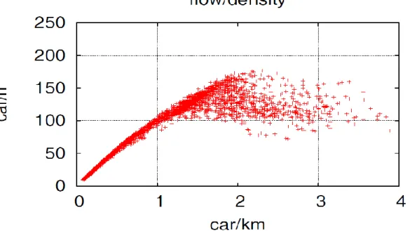
Figure 4.Flow-density plot from real-world traffic data, these are taken from the “grande raccordo anulare” in Rome
Most real world data collections yield graphs very similar to the one in figure 9 above, the free-flow branch can be easily identified, but after the critical density it is very hard to define a proper curve.
1.4 Phase transitions
The notion of a phase transition might seem inappropriate on the topic of traffic, some statistical mechanics purists would say that rigorously speaking there are no possible phase transitions in traffic, since there is no sensible way of defining a partition function, the system is open, and somehow never in a real equilibrium condition, and even more important, the number of particles and the system volume have no way of going anywhere near infinity.
By analogy with empirical experience, a phase transition will be defined here as the point where a small change in the value of a control parameter of the
18
system, causes a significant change in some macroscopic variable we are measuring. For every practical application in the rest of this chapter the number of vehicles Ncar on a network of fixed dimensions, will be used as a control
parameter and the flow Ncar<V> will be measured and recorded as a
macroscopic variable of interest.
Flow-density plots have been in the past the most widely used graphs in traffic studies, along with speed-density plots and flow-speed, graphs are of course linked by the equation =v
Traffic, according to some theories is believed to have two or three different phases
I. Free flow. It is somehow analogous to the gaseous phase in thermodynamics; this is the phase in which the effect of interactions between vehicles are not dominating the dynamics, cars go as fast as drivers wish to go, compatibly with legal regulations and road conditions, the dynamics is weakly dependent on the interactions between vehicles.
II. Synchronized motion: The existence of this phase has been part of an intense debate in academic papers on the subject, being somehow analogous to liquid phase, and as such is an intermediate condition between the free-flow and the congested phase in this state cars are moving synchronously at speeds way lower than the limits imposed by the law or the characteristics of the road, it has been somehow observed in highways, whether this is a robust phase is still an open question.
III. Congested state or wide moving jams. The term wide is used though of course it refers to the length of the jam and not to its width, analogous to solid phase, the interactions between vehicles strongly dominate the behavior of traffic, the motion of traffic in this situation is usually characterized by stop&go waves propagating backwards
19
Most of the studies on the traffic phases focus on the collective dynamics of a single long road, this does make sense, since for sure it is the system that can more easily be studied, the effects of small changes in the dynamics parameters can be readily addressed, and many variables can be studied in detail. This is the first step toward the investigation of more complex road network, this will be the focus of later chapters.
1.5. A brief review of car following models
Understanding drivers behavior is of course key in devising a performing traffic simulation; car following describes how a pair of vehicles on the same lane interact, and plays a major role in determining the accelerations and the mutual distances between vehicles in the model.
There is a number of factors influencing car following behavior, usually classified in 2 different categories, the first category are those depending on the individual characteristics, such as driver's age, gender, risk taking behavior, vehicle performance; the other category includes those situational factors that involve both the individual and the environment, such as stress, fatigue, alcohol or drugs intoxication, road conditions, weather or other possible distractions, such as other people in the vehicle or eye catching ad billboards.
Reliably representing in a model environmental effects is hardly feasible, and even measuring and quantitatively evaluating the influence of those on the driver behavior is beyond the possibilities of a model, but stable individual differences can be reasonably modeled on empirical data, drivers over 59 years of age seem to prefer a headway 23% greater than drivers of an age ranging from 23 to 37 (Evans and Waasieleweki, 2003) , also males are reported to choose on average a shorter headway than females.
20
a. the Gazis-Herman-Rothery models (GHR);
b. the Safety-distance or collision avoidance models (CA); c. the Linear models (Helly);
d. the Psychophysical or Action Point (AP) models; e. the Fuzzy logic models
The Gazis-Herman-Rothery models (GHR).
These models, developed in the late 50s in the General Motors labs are based on the equation:
𝑎𝑛(𝑡) = 𝑐𝑚(∆𝑣
𝑛(𝑡 − 𝑇))/(∆𝑥𝑛𝑙(𝑡 − 𝑇))
where a is the acceleration of the vehicle of interest, ΔV is the difference in speed between the vehicle and the one immediately ahead of it, ΔX is the distance between the aforementioned vehicles, t is the current time, T is the driver reaction time, m, l and c are model calibration constants determining which is all but trivial, there have been many possible estimates, mostly based on closed-track experiments, but still there is no widespread consensus regarding the values of such parameters.
Safety-distance or collision avoidance models (CA).
These models date back to 1959, from the work of Eiji Kometani and Tsuna Sasaki. The CA models, unlike the GHR do not specify a stimulus-response type function, but they seek, trough manipulation of Newton's basic equations of motion, a way to specify a safe following distance, within which a collision would be unavoidable as expressed by the original formulation:
∆𝑥(𝑡 − 𝑇) = 𝛼𝑛−12 (𝑡 − 𝑇) + 𝛽𝑣
21
where Δx as before is the distance between the nthand the (n-1)thvehicle, t is the time, T is the reaction time, b0 is the braking capability of the vehicle, V is the speed of the nth vehicle, α, βand β1 (as of course are T and b0 ) are
parameters to be determined experimentally, just as in the GHR model.
Linear models (Helly).
These models, that also date to 1959 are usually attributed to Helly although the GHR model too was originally based on a linear relation, it is based on the following equations:
𝑎𝑛(𝑡) = 𝐶1∆𝑣(𝑡 − 𝑇) + 𝐶2(∆𝑥(𝑡 − 𝑇) − 𝐷𝑛(𝑡)) where D, the desired following distance is defined as:
𝐷𝑛(𝑡) = 𝛼 + 𝛽𝑣(𝑡 − 𝑇) + 𝛾𝑎𝑛(𝑡 − 𝑇)
This model has quite some similarities with the GHR model, most of the simulation work in this chapter is based on a variation of it, it is different of course from a collision avoidance model, but it allows to easily tweak the safety distance, since it appears explicitly in the equation.
Psychophysical or Action Point (AP) models.
Not as easy to describe with a straightforward equation as the others, but for sure worth noticing are the psychophysical models, also called action point models. These are based on the assumption, first suggested by Michaels in 1963 that a driver can tell if the distance with the preceding vehicle is changing if he sees a noticeable change in the apparent size of the vehicle, in other words the driver perceives the change in speed of the preceding vehicle as changes in the visual angle θ subtended by the car ahead. The threshold is known to be (Δ v/Δ x2)∼6∗10−4when this threshold is
22
exceeded, drivers will choose to decelerate until they can no longer perceive a relative velocity, and if this threshold is not re-exceeded they will base their decisions on the perceived changes in spacing.
Fuzzy logic models.
A fuzzy logic model is used to describe the behavior of a driver, a human being that is likely to make decisions based on more than a single input variable, a fuzzy logic based model combines many different input variables into a fuzzy set, where the information will be used to assess the level of truth of some binary variables such as “close”, “too close”, “closing”. They offer a very realistic looking approach to modeling traffic and they undoubtedly have plenty of potential, there is much research being made, but none of the commercially available traffic simulators today are based on fuzzy logic.
23
1.6 What to do: a Physicist's standpoint
The choice of the model to use for simulating traffic behavior is a critical decision; as previously stated, traffic is a complex system, and as such, we don't want the model to oversimplify the problem, a physicist would be tempted to use a model he can easily understand and manipulate, but as a smooth sphere is not a proper approximation of a horse, using a simple model exposes us to the risk of removing those critical features of the system that are responsible for the emergent properties that we are mostly interested in understanding, on the other hand we want the model to be as simple as it can be, for computational speed and also for making it feasible, once in a while to find analytical solutions in simple cases. There is of course no right and wrong choice in general; a model very suited to solve a particular problem could be completely unfit to tackle another.
Calibration itself, and the tuning of the model is also an issue; as mentioned before, it is possible to introduce a large number of features in every single agent of the model, there are models that describe the acceleration taking into account gear changes, the torque curve of the engine, and countless other features, but doing so would quite drive us away from the goal: in reality we have no way of reliably and deterministically describing the behavior of a human being driving a car, we have no way of knowing what car will be where and when, and whatever estimate we make of these features will carry such large errors to be of no quantitative interest or so.
24
1.5 The model: Mobilis
The model used here is called Mobilis, it is a software developed in the physics of the city laboratory at the Alma Mater University of Bologna. It is entirely developed in C++, it is for our purposes a single lane car following model, so there is no overtaking taken into account, this might seem like a big approximation, but it turns out to be more than adequate at reproducing quite faithfully many traffic features.
The model can be used to build a model of a road network, taking in consideration various possible regulations of intersections; such as left or right yield, traffic signals, roundabouts, forced turns, or one-way roads; the model in action can be monitored thanks to a fltk based graphic interface. Many traffic features on different network configurations have been analyzed, testing the performance of the model against proven results of the theory and investigating new features where possible.
25
Figure 5. A Manhattan/chessboard-like road network as represented in the Mobilis Software. It is called Manhattan because of the square grid shape, and chessboard because of the alternating crossroad junctions and roundabouts. This configuration has interesting unique properties.
26
Figure 6. A 2-way road as it is represented in Mobilis
1.5.1 The characteristics of roads in the Mobilis Model
In Mobilis roads are built as 2 non interacting lanes of width 3/2L, where L is a scaling parameter, usually equal to 4 meters, in the middle of every lane there is an L wide are where cars are moving, leaving in each lane an L/4 free area on the sides. No overtaking or U turns are considered, so there is no interaction between cars on different lanes, for making it easier to easily spot higher density areas the color of every lane changes with density, from blue in case of very low density to red when density is very high (usually in that case the road is congested already).
1.5.2 Nodes in Mobilis
Nodes are divided in 2 categories: external nodes and intersections. External nodes usually play the part of sources of sinks for the agents of the model, though agents could if needed be created or destroyed in any node; the agents are created in the external nodes, which are displayed only as a road with an open end, and from there they move towards their destination, following the algorithm they are supposed to follow in that specific simulation. Intersection nodes are also divided in 3 and 4 way intersections, and 3 and 4 ways roundabouts.
Intersections can be regulated in various ways; there can be a traffic signal alternating green and red phases, the timing for each signal can be set
27
independently
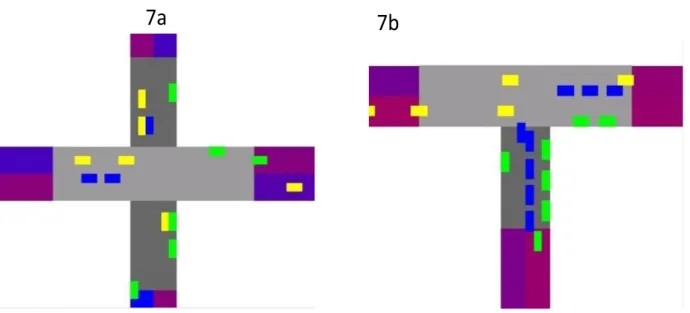
Figure 7. Left side (7a): A 4-way intersection, the road with the darker shade of gray is the one that has to yield in case of no signal, and the one that has a red light if the signal is active. Right side (7b): A 3-way intersection, the meaning of the shades of gray are the same as in the 4-way intersection.
Rundabouts on the other end have no need for such regulations, in real life they seem to be dominating most of road planning in European cities, their effects on the global dynamics of a road network cannot be neglected,
28
Figure 8.A roundabout in Mobilis, its functioning replicates quite faithfully the ideal behavior of a real world roundabout
The structure of a roundabout in the model is quite complicated; the inside of the roundabout is built as a 3-lane circular road, so, cars going straight, left or right have their own lane to use in the roundabout, cars trying to enter the roundabout of course yield to those that are already in. As we shall see later, roundabouts allow for self-organization of traffic, whether this is more or less efficient than an old-fashioned traffic signal strongly depends on traffic conditions.
1.5.3 Car following dynamics
The car following equations used in these simulations are not based on any of the models described in the previous chapter. The reason for this unorthodox approach is simple; while those dynamic models presumably can reproduce
29
urban mobility dynamics in a quantitatively reliable way, that is not the purpose of this work. Many different car following models were tested in a single-lane model, just to see if they produced phenomena of interest (stop&go waves propagation namely). All the models discussed before can recreate this type of traffic behavior, but they all have many parameters and overly complicated equations for our purposes. The model chosen is a linear model with a safe-distance that depends on the second order of speed, dependent only on one parameter.
Figure 9. Screenshot of a one-lane simulation used to test different dynamics
When the distance from the preceding car is greater than the safety distance, the car accelerates trying to reach the maximum speed allowed on the road it is on, following the equation:
𝑎𝑖 = 𝛼(𝐶𝑣𝑚𝑎𝑥− 𝑣𝑖)
where ai and vi are the acceleration and the speed of the ith vehicle, α is the
acceleration parameter, relative to the supposed performance of the car, Vmax is the maximum allowed speed and C is a parameter relative to the local curvature of the road.
The safety distance is defined as
𝑑𝑠 = 𝑑𝑚𝑖𝑛 + 𝑇1𝑣
is a calibration constant relative to the stopping distance, it has the
30
linear approximation of the safe distance it is quite effective at giving reasonable qualitative results on many networks below critical densities; whenever the purpose was to study the phase transitions or the behavior of the simulation in high density conditions, a quadratic term was added.
𝑑𝑠 = 𝑑𝑚𝑖𝑛 + 𝑇1𝑣 + 𝑇2𝑣2
The parameter T2 allows also to take into consideration different driver behavior,
this will be done in the calibration by changing the value of 𝐷2 = 𝑇2∗ 𝑣𝑚𝑎𝑥2
When the distance from the preceding car is lower than the safety distance, the car follows the equation:
a
i=γ∗(D
ij− D
s)
where is a calibration parameter, which value whose chosen to simulate the empirical fact that a road car has much better braking than acceleration.
This model shows phase transitions both on single roads and larger scale networks.
1.8 Analysis of some test networks
1.8.1 A single ring
31
Quite some time was devoted to analyze the characteristics of the fundamental diagram in some sample networks: the first test was done on a single closed ring. The ring, was composed of 4 roads, placed in a square, connected by 4 roundabouts, cars were proceeding counterclockwise, so they had to go all around every roundabout, this is irrelevant for this experiment, since the ring is isolated, but it will be important when the ring will be interacting with other traffic structure. The distance between the centers of the roundabouts is 600 m, every roundabout has a radius of 30m, so a single loop of the ring is 2725m. I first tried to see how the fundamental diagram looked in this simple case. The graph is generated as a series of 20 simulations each 4 hours of simulation time long, the flow is calculated as the average speed of all cars in the equilibrium state which reached quickly after all cars have entered the ring. To remove all the effects of transients from the data, all the output from the first hour of simulation was discarded.
32
Figure 11. Flow density plot on a single ring.
This looks very similar to the triangular fundamental diagram, which is generally acknowledged to be closer to experimental data on single lane roads than the bell shaped one. The density can get very high without the system entering a lockdown. Looking at the simulation, in the free flow branch cars proceed undisturbed or so all along the road; at densities higher than the transition point, stop&go waves start to form, usually a single one propagating backwards along the whole ring; all that changes raising the density is the amount of cars that are stuck in the stop&go at the same time.
Being this single ring structure very simple, perfectly equivalent to a single road with periodic boundary conditions, it was ideal for studying the effects of the parameter D2 in the safe distance. The parameter was chosen so that the safety
33
distance couldn’t get smaller than dmin therefore, taking the safety distance
equation
𝑑𝑠 = 𝑑𝑚𝑖𝑛 + 𝑇1𝑣 + 𝑇2𝑣2
We need to impose 𝑇1𝑣 + 𝑇2𝑣2 > 0 for every 𝑣 < 𝑣𝑚𝑎𝑥
Therefore 𝑇1𝑣 > |𝑇2𝑣2| → 𝑇
1𝑣𝑚𝑎𝑥 > |𝐷2|
imposing 𝑇1 a headway of 2 seconds, and given 𝑣𝑚𝑎𝑥 = 13.9 𝑚/𝑠 (60 𝐾𝑚/ℎ) yelds
𝐷2 > −27.8
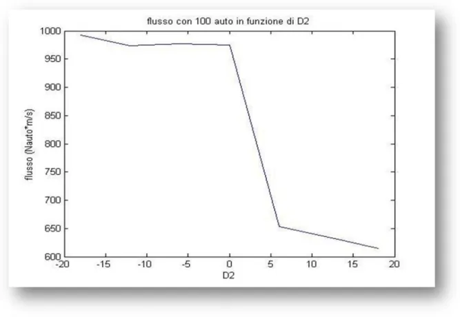
A series of simulations were run with a fixed number of 100 cars which were enough to make stop&go waves appear independently of the parameter, to evaluate the average flow in a 4 hour run for every integer value of the parameter between -18 and +18 meters. Cars with a negative value of the D2
parameter are way more efficient, due to their choice of a shorter safety distance , and the ones with a positive value are more careful drivers, choosing a higher headway the next logical question then was about the effects of mixing drivers with a positive D2, with some with a negative D2.
34
Figure 12. Flow of 100 cars on a single ring varying the value of the D2
The simulations were conducted the usual way, the differences in flows, though not dramatic show that positive D2 makes for slightly higher flows in the
free-flow state and sensibly lower free-flows in the congested state and the interesting property that the mix of the two seems to behave slightly better than both the homogenous systems.
No extensive microscopic traffic data are available in order to make a better calibration of the parameters, so the choices of the parameters values of D2
between +12 and -12 meters has been used as a reasonable way of creating some diversity in driver behavior. In all subsequent simulations the D2parameter
35
Figure 13. Another fundamental diagram on the same single ring: the blue line is the flow when there are only good (negative D2) drivers, the purple one is done with only bad (positive D2) drivers and the green one with an equal mix of good and bad drivers
1.8.2 Two interacting rings
In the previous example there was no interaction between cars on different roads. This happens at intersections. This simple model it is composed of two of the rings of the previous paragraph linked by a roundabout.
36
Figure 14. Two rings connected by a roundabout.
Since all cars go counterclockwise in the roundabout, whenever this is occupied they have to stop and yield; cars on one ring never move into the other. The number of cars in the first ring was fixed to 80, which were proven in the previous paragraph to be not enough to generate stop&go waves. If undisturbed, cars in ring one would remain a steady free-flow state. A series of simulations varying the number of cars in the second ring were made, up to making them equal in both rings.
37
Figure 15.The flow-density plot on two interacting rings: in blue the flow on the first ring, constantly occupied by 80 cars, in green the flow in the second ring with a number of cars varying from 10 to 80 in red the sum of the two flows.
This looks nothing like the fundamental diagrams showed before; but this is nonetheless part of the fundamental diagram of the network; it appears there is an upper limit to the number of cars that can get through the roundabout in a given time, somehow analogous to the rate of flow in a pipe in fluid dynamics, which is even more evident watching the sum of the two flows, which apart from a slight decrease in the left part of the graph, probably due to the effects of interactions having an effect somehow analogous to viscosity or drag, turns out to be approximately constant. Looking at the simulation it is evident that the behavior of the stop&go waves is a lot different from before, if in a congested single ring steady stop&go waves formed, here the roundabout becomes a source of many waves, travelling upstream, at high enough densities in both rings, but the roundabouts completely breaks the regularity of such waves, a wave forming in one ring gets to the beginning of the cue starting at
38
the intersection and dissipates. Increasing the number of cars in both rings doesn't give any significant change, putting 100 cars in one ring, slightly more than enough to cause stop&go waves to appear spontaneously and raising the number of cars in the other to 100 too, the behavior of the system looks much similar to the previous one.
Figure 16.The flow-density plot on two interacting rings: in blue the flow on the first ring, constantly occupied by 100 cars, in green the flow in the second ring with a number of cars varying from 10 to100 in red the sum of the two flows. There seems to be no significant change in the behavior of the model from the previous simulations.
1.8.3. A Manhattan-like road network
Though this is somehow just another test network, its importance and greater complexity makes it worth a deeper analysis;
39
roads intersect each other at a 90° angle, forming a large grid of mutually intersecting roads, we called it Manhattan, but Turin, Barcelona and many other cities exhibit similar layouts. The reason this kind of map in a city is so common goes back to the Roman Empire and their idea of urban planning.
The characteristic of such a road network are way more complicated than the previous examples, but it offers a chance to investigate the effects of larger scale interactions between multiple crossroads and/or roundabouts. In this model intersections are placed at a distance of 200m from each other, and the external nodes are 200m away from the adjacent internal nodes.
Figure 17. A small Manhattan-like road network with simple intersections and randomly timed traffic signals
Unlike the previous models, this one is open, cars can leave the network through any of the external nodes, which are of course also the ones trough which they enter the simulation, the decision making is pretty straightforward, at every crossroad every car determines randomly which direction to take; this is very unlike real traffic, but brings the system closer to its thermodynamic analogs, under such conditions the probability space is homogenous and the
40
characteristics of the road network can be investigated without bothering with individual choices or origin-destination matrixes.
Studying the fundamental diagram is trickier than in the previous cases; keeping the number of cars constant at high densities without having the whole network fall in an irreversible lockdown, due to the agent intelligence shortcomings, is quite challenging, and getting a smooth averaged plot is almost unfeasible. In order to make the simulation proceed it was necessary to monitor the average speed and the density for the whole duration of the run, making sure the system didn't go in an irreversible lockdown adjusting manually the rate at which the external nodes put cars in the system.
The shape of the Flow-density plot that came out of this process was much different from the one expected (Fig. 18).This kind of behavior was not easy to
explain at first; In many fundamental diagrams obtained from experimental data there are points that appear way below the expected point in the density-flow curve, but there was no explanation for these outliers other than the inherent complexity of the system and the network on which the experiment was performed. A recent paper (Geroliminis et al 2011) on the topic gives a
promising explanation. In that paper they analyzed some real world traffic data from the network of highways in Minnesota, and showed how the system
seemed to have some memory of the previous states, making another
thermodynamics or solid state physics analogy, cars in a road network show an Hysteresis like behavior.
41
Figure 18. The Manhattan-like network with traffic signals. Flow-density plot from the simulation. From A to B the free flow branch, from B to C the decreasing branch, from C to D an Hysteresis branch.
Even if the fundamental diagram keeps being a property of the network only, independent from the number of cars in it, at a given density there are various possible flows; once the system is congested, if the demand suddenly decreases it doesn't return to its free-flow state going back through the peak, but it goes through an hysteresis cycle. There are various possible explanations for this behavior, in the aforementioned paper the main hypothesis was that this kind of phenomena was mostly induced by spatial inhomogeneity in the demand, which is not the case in my simulation since cars are introduced from all nodes at equal rates and decide where to go in a completely random fashion, the inhomogeneity here is in the time change of the demand; when the system is highly congested the amount of cars entering the system is sharply dropped, so given a little time the network slowly “decongests” itself closing the Hysteresis loop in the figure above.
There is still no proper theoretical explanation of this behavior of traffic in a network, but there are some interesting points to examine. When the simulation
42
is going through the lower branch of the loop, the density is highly non homogenous, there are some congested blocks, while all the other roads are in a free flow state. This, in more detail will be the topic of the next chapter.
1.8.4 A Manhattan-like road network with roundabouts
The previous model was regulated by traffic signals, in recent years much emphasis has been put on roundabouts, as they allow traffic to self-organize, without introducing any artificial timing in the system.
Figure 18. A Manhattan like network with roundabouts
Roundabouts are expected to make the network perform way better in the free flow branch, but their behavior in a congested scenario could be very far from optimal
43
Figure 19.Flow density plot on a Manhattan network regulated by Roundabouts
The system enters an irreversible lockdown with little or no warning; the appearance of congestion completely kills the system dynamics very quickly.
Figure 20.Lockdown configuration of the roundabout network
As shown in the figure, closed loops form between roundabouts, so that they depend on each other in order to move again. Real traffic wouldn’t of course be completely and irreversibly locked, but would for sure be in a very low flow condition, relying exclusively on drivers’ goodwill to get back moving.
44
1.8.5 A “chessboard” Manhattan Network.
It seems clear looking at the previous paragraphs that roundabouts are more efficient than signaled intersections in low density conditions and less efficient when congestion starts to arise. A intermediate solution of course is feasible.
Figure 21. A Manhattan/chessboard road network
This is the same configuration shown in Fig. 5 at the beginning of the chapter; it has been named the “chessboard” because signals and roundabouts are disposed like black and white on a chessboard. Signals on one row are opposite in phase with the ones in the other, therefore the idea is to regulate entrances in the roundabouts, so that the local density doesn’t get critical too soon.
45
Figure 22.Flow-density plots of the three similar networks. In green the roundabouts only one, in blue the chessboard one, and in red the uncorrelated signals one.
When comparing the behavior of the three similar systems it seems clear that the chessboard has a slightly longer free flow branch than the other two, while the roundabouts only one performs better than the other two on the free flow branch, especially at low densities. When densities get higher, the performance differences get smaller, and the signals only system is the only one capable of getting through an hysteresis loop and going back to the free flow branch if the external flows are reduced, while the others inevitably fall towards a lockdown when density gets critical. The free flow branch in the roundabouts network resembles more than the others the curve expected in a single lane fundamental diagram, since there are no signals disturbing the self-organization of cars.
46
2.
Hysteresis phenomena and phase
transitions in ideal urban mobility
networks
2.1.The model and the fundamental diagram
In the previous chapter the topic of phase transitions and hysteresis emerged from watching the shape of fundamental diagrams in microscopic simulations. The characteristics of the networks there though didn’t allow for some solid statistics, the biggest model that was investigated was a four-by-four Manhattan network. The fundamental diagram here would be better called a “macroscopic fundamental diagram”; historically flow density plots have been used to characterize the behavior of single roads, typically highways; It has been shown however (Geroliminis et al 2007) that interconnected road networks might follow a unique macroscopic fundamental diagram. To do so a bigger Manhattan network was built; a ten-by-ten network, with 100 crossroads regulated by uncorrelated traffic signals and 40 external nodes (Fig.23).
47
Figure 23. 10-by-10 road network as used in the simulations
As before, the system is open; cars can leave the simulation by going through any of the external nodes, which are also the sources that generate the cars in the model. It is not therefore possible for now to control directly the number of cars in the system, with this setup, what is controlled is the inflow; the number of cars that enters the network every second trough each node which is set to be equal for every source.
Various simulations have been run on this network to explore the statistics of the possible states it can go through.
48
Figure 24. Rescaled flow-density plot and density variance on one run
Figure 24, though obtained by a single run, shows clearly the connection between the phase changes of cars in the network and the variance of density on the roads: when the number of cars is increasing variance slowly but steadily increases, as flow reaches its maximum, the system makes a transition to a congested state, variance sharply increases, flow goes through a clockwise loop, showing hysteresis behavior as in the smaller model, while the variance loop goes counterclockwise; the congested hysteresis branch clearly shows a much higher density variance then the free-flow state, as expected.
2.2The density distribution
Since the density variance and the flow seem to show some meaningful correlation, the next step was investigating the density distribution in the various states, identifying the states from their respective positions in the fundamental diagram plot. First of all a few runs were made keeping the incoming flow low enough so that the system could remain in a free flow quasi-equilibrium state indefinitely.
49
Figure 25. Density distribution histogram in various free flow quasi-equilibrium conditions. The flows are intended for every single external node.
If the incoming flow is low enough then the density distribution closely resembles an exponential decay, as expected, when flows increase, a peak appears, and it shifts to the right and gets broader as the external flows, and therefore the densities increase, just as the density variance plot in the previous figure would suggest. Studying the decreasing branch of the fundamental diagram is not an easy feat, it is very hard to keep the simulation in that condition stably; the flow maximum seems to be a metastable state, from which it can drop to the mixed phase equilibrium value following a vertical trajectory in the flow-density plot. The decreasing branch of the fundamental diagram is rarely observed in real-world data, and in this the simulation is very lifelike. The density distribution histograms in Fig. 26 gives us a clearer understanding
50
that the congested state the system enters once it gets past the maximum is a mixed state, therefore, if some other thermodynamic analogies hold, it should be a 1st order phase transition. The graph shown in Fig. 26 is derived from a
series of time slices taken while the system slowly relaxes to a free flow state from a highly congested state. It is clear looking at the picture that the road population splits between roads that keep following roughly the free flow statistics and roads that have a density very close to the maximum. In the beginning, the high density peak is higher, and few roads are in the free flow state, as the system decongests roads go from one state to another, getting in the end to a distribution very similar to the one of in the free flow state.
Figure 26. Density distribution histograms along the hysteresis/mixed phase branch, data 1 is relative to the rightmost and more congested part of the branch, the following are relative to the progressively less congested system as it goes back to the free flow state.
51
2.3Back on the macroscopic fundamental diagram, conjectures on phase transitions
There has been quite some work on the characteristics of the fundamental diagram; many studies focused on the characteristics of the decreasing branch, Boris Kerner [7] introduced the three phase traffic theory as a qualitative model to describe traffic behavior when interactions have a strong effect on the dynamics.
Since the macroscopic fundamental diagram is a property of the network (Daganzo et al 2008), there is little point in discussing the general shape of it, even if it is just a numeric simulation, the 2 ring example in the previous chapter shows clearly that the geometric characteristics of the network and the intersection regulations can drastically change its layout. The early fundamental diagram from Greenshields referred to a single highway, there are however experiments on whole cities, such as Toulouse, France and Yokohama, Japan (Geroliminis et al 2011) that show an empirical density-flow profile that is in some regions very similar to the single lane model one, including also a clockwise hysteresis loop that is much similar to the one shown in the previous paragraph, but also many experiments that show a completely different behavior even just on larger regions of a single highway.
52
Figure 27.Another flow density plot on the “Grande Raccordo Anulare” in Rome. In this some hysteresis-like behavior can be observed in the lower region, but on the whole it is very difficult to define a slope after the traffic breakdown.
The work from Kerner (Kerner et al 1997) theorizes a change in the slope of the descending branch of the fundamental diagram, and though the theoretical calculations are for sure correct and probably do apply in some real-world scenario, it is hard to get such accuracy in the measurement, and the equilibrium condition such models refer to is not very descriptive of real road networks. In most fundamental diagrams sketched from empirical data there is no evidence the descending branch of the diagram has a defined slope at all. In the Mobilis simulation, if the average density is kept stably at a value slightly lower than the one corresponding to the expected flow maximum the system collapses to a mixed state after a short time.
The simulation run up to now, except the one in the figure 28, were done controlling the incoming flow, but no constraint was put to the number of cars in the simulation. This did account well for the study of the network responding to different traffic demands, but does not give us any information on the stability of the various states in the fundamental diagram at different densities. A series of runs were made then, controlling the density, and except for some transients,
53
left there long enough to investigate the stability of the state.
Figure 28.Transition from free flow to a mixed state at non critical average density To further understand the behavior of the fundamental diagram of this system there are two different roads to take; one is studying the system at constant density, and the other is studying it at constant input flow.
Constant density
The flow-density diagram, if gone through slowly increasing the density, looks nothing like the usual bell shaped curve, if the desired density is lower than a critical value, flow is a monotonously increasing function of density as in the single lane model; average speed is decreasing along the branch, but the points in the plot are very far from the hypothetical maximum flow line because traffic
54
signals have a strong impact on average speed. Interactions between vehicles are present even at these densities, but can be neglected.
Figure 29. Sketch of the flow-density diagram in the simulation.
Increasing the density further (entering the teal region of the graph in figure 29) the flow keeps increasing linearly or so, until density gets high enough to make a transition to a mixed state. The transition here is quite abrupt, and can easily be identified watching the simulation. While in the linearly growing branch road occupancy was homogenously increasing, now there are one or more clearly congested areas. Density can be set even at higher values, flow will stay on the “nearly” constant red line in the graph until it reaches a region where a transition similar to the one before can take place, taking the system in an irreversible lockdown. In this state there is typically one huge congested area that will survive indefinitely. Even if incoming flows are set to zero there will be no going back to the previous condition, this specific behavior is somehow an artifact induced by the model; it happens as some congested structure forms a closed loop, and it creates a chain of interactions long enough that a loop of static congestion can be closed.
55
Figure 30.An irreversible lockdown in the model
If when the system has entered the mixed phase density is decreased, it will go back to the linear branch closing the hysteresis loop. All points there are stable at fixed densities, there are no “vertical” transitions allowed far from the area where the mixed-congested branch meets the stable free-flow branch, and in simulations there are no vertical transitions from the free flow branch to the mixed state below some critical density. Changing the system density gives rise to transients effects; for all the simulations in figure 31, the system was kept from time to time at a density locked between two boundaries, oscillating from maximum inflow to no inflow. This caused some counterclockwise loops to appear in the free flow branch, as in the rarefaction phase flow increases significantly.
Constant inflow
If the inflow is kept constant the system moves on the same plot in a slightly different way. If the flow is lower than a certain threshold value, the system will reach a point of equilibrium in the density-flow plot somewhere along the stable free-flow branch, if the inflow is above that threshold, the system will dynamically go through a path that resembles a bell shaped curve (the green part in the graph), will make a transition to the mixed phase, and then to the lockdown zone after some time, unless the inflow is significantly reduced.
The maximum inflow that allows the system to dynamically cross all the mixed phase backwards is approximately the same flow that would allow a stable
free-56
flow condition in the area where the two lines meet, empirically 𝜌 ≈ 𝜌𝑐𝑟𝑖𝑡/2.
If the flow is higher than that, the system will unavoidably make a transition to a complete lockdown after some time. This maximum inflow is clearly related to the outflow from the congested “cluster” which seems approximately constant. All along the hysteresis the cluster size decreases, as the density distribution plots some pages ago showed.
Going back to the thermodynamic analogy, it seems, as mentioned before, this has much in common to a first order phase transition; where the two end states are the free flow state and the lockdown state, the congested state, along the hysteresis branch is a mixed state, similar to freezing water. Like water, it can get to a state that resembles super cooling, which is the higher part of the free flow branch; the density is more than high enough to allow, if kept constant, a congested cluster to survive, but it’s not high enough to allow a “homogeneous nucleation” of a congestion. The density is such that if some big enough disturbance occurs, it would cause a group of cars to slow down and create a cluster, but it’s not high enough to allow smaller clusters forming spontaneously out of the system random oscillations to become nuclei for the formation of a bigger cluster. In the hysteresis branch on the other hand, one or more big clusters have formed already, and they can either be kept at a stable size, grow up to a complete lockdown or shrink down and disappear, depending on how the density of the system is controlled.
57
Figure 31. Various density plots superimposed, in different dynamical states.
2.4. Scale dependencies
All the previous simulations were done keeping the size of the system constant, the distance between intersection was 200m for all simulations, in order to study a similar system at different scales, quantities have be normalized; the following plots will be 𝜑 − 𝑘 plots, where
𝜑 = 𝑘 ∗< 𝑣 >
In this framework, a few simulations were run to study the behavior of a network twice the size of the first one, the distance between nodes is 400m.
58
Figure 32.Normalized flow-concentration plot on the smaller network (blue) and in the
one twice the size (green).
Keeping the density close to constant by having it oscillate between two
extremes makes the plot very noisy, there is plenty of non-equilibrium effects, rarefaction-compression loops and similar trajectories, that are interesting for the description of the dynamics but are not the purpose of this study.
The simulator was re-run to get a more defined quasi equilibrium plot on both scales (Fig.33); to do so, density wasn’t set to oscillate between two extremes as before, but it was slowly increased and then decreased when it reached a value close to the irreversible congestion, to follow and analyze all states in the diagram as close as possible to a constant density condition.