UNIVERSITA’ DEGLI STUDI DI PISA
The effects of index rebalancing:
an empirical evidence from the Italian market
Academic year 2012-2013
Course in Finanza Aziendale Mercati Finanziari
Supervisor
Prof. Roberto Barontini
Student Muça Vera
Index
Acknowledgment ... 4
Introduction ... 5
CHAPTER 1. CAPITAL MARKET THEORIES ... 8
1. The foundation of modern capital market theories ...8
1.1 Efficient Market Hypothesis (EHM) ... 8
1.1.1 The Three Forms of Market Efficiency and Behavioral Finance ... 10
1.2 Event Studies and Market Efficiency ... 11
2. Asset pricing in an efficient capital market – The Capital Asset Pricing Model ... 12
2.1 Assumptions of the CAPM ... 12
2.2 The Fama and French three-factors model ... 14
3. The liquidity premium ... 15
Chapter 2. Empirical studies regarding market efficiencies and index variation . 19 1. The Predictions of the Efficient Market Hypothesis ... 19
1.1 Market Inefficiencies ... 21
1.2 Behavioral Finance ... 24
2. The Fama and French Empirical Study Regarding The CAPM’s Invalidity ... 25
2.1 The Bad Model (The incompleteness of the CAPM) ... 25
2.2 Consequences ... 26
3. The hypotheses that explain the index effect ... 27
3.1 The Price Pressure Hypothesis (PPH) ... 27
3.2 The Imperfect Substitutes and the Downward-Sloping Demand Curve for Stocks ... 28
3.3. The Liquidity Cost Hypothesis (LCH) Hypothesis (DSH) ... 29
3.4.The Information Content Hypothesis and the Certification of an Index Member (ICH) ... 29
3.5 The Market- Segmentation and Investor Recognition Hypothesis (IRH) .... 30
Chapter 3. An empirical evidence from changes in Italian indexes’composition ... 31
1. The objectives of the analysis ... 31
2. The Event-Study Methodology ... 32
2.1 Steps on the typical Event-Study ... 33
3. Evidence from changes in Italian indexes ‘composition ... 35
3.1 The selection and management process of the three indexes (S&P/Mib FTSE Mib and FTSE Italia Mid Cap) ... 35
3.2 Data ... 39
3.3 The methodology ... 43
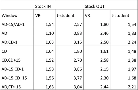
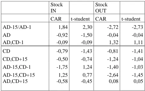
4. Result interpretation ... 45
4.1 Price and volume effect for S&P/Mib and S&P/Mib ... 45
4.2 Price and volume effect for Midex and FTSE Italia Mid Cap. ... 50
Final Conclusions . ... 56
References. ... 59
Acknowledgments
It would not have been possible to write this thesis without the help and support of the kind people around me, to only some of whom it is possible to give particular mention here.
Above all, I would like to thank my mom for believing in me and supporting me in every step of my live, my sister “Lilushi” for her support and great patience at all times, my grandparents and all my relatives especially ‘’Kikushi’’ who has been an excellent example to follow and all the others who have given me their unequivocal support throughout, as always, for which my mere expression of thanks likewise does not suffice. A great acknowledgments goes to my uncle Dino and his wife Entela who have supported me in the most difficult moments at the beginning of my studies here in Italy and to all the others uncles in Albania and Greece.
This thesis would not have been possible without the help, support and patience of my supervisor, Prof. Roberto Barontini, to mention his advices, his encouragements and his availability in every step of this thesis and also for his help in directing me in a post – graduating program ‘‘Master Mains’’.
It would not be fair not to mention Prof. Davide Fiaschi who has always believed in me and supporting me in my decisions.
Finally, all my friends Klesti, Livia, Rezi, Tixhja and in particular Jola with whom I have divided almost every single lesson, exam, difficulties, studing hours ecc. To be mentioned are the girls at ‘‘Praticelli’’ and ‘‘le bimbe di FAMF’’ who have supported and helped me along the course of my studies at ‘‘Facoltà di Economia’’.
Introduction
In the last 50 years the financial literature has revealed numerous empirical anomalies, pointing out the inconsistencies of some traditional models (CAPM) and efficiency hypothesis (EMH). Hence, the modern financial literature, taking into consideration those empirical anomalies, has proposed a vast number of explanation regarding this issue. So, the main purpose of the financial literature is to explain the principal limits of the traditional approaches based on complete information and investors that take their decision rationally.
All the modern Capital Market Theories, in particular the EHM, are able to explain the empirical anomalies regarding the abnormal returns and trading volumes due to index change if that fact provides new information to the market. The principal view of capital markets adopt the ‘’perfect-world’’ scenario where markets are perfectly efficient and the asset prices quickly and accurately reflect all the new information available in the market. So, asset prices in an efficient market ‘fully reflect all available information’ (Fama 1991). This implies that the market processes information rationally, in the sense that relevant information is not ignored, and systematic errors are not made. As a consequence, prices are always at levels consistent with ‘fundamentals’.
Despite adopting a ‘’perfect-world’’ scenario, some inefficiencies and anomalies are not yet explained by the traditional models in absence of new information (e.g. the abnormal returns), hence it is quite interesting to gather this opportunity and conducting this study, pointing out the effects of index rebalancing. Among the events that the traditional models are not capable to explain, is the case of abnormal returns/trading volumes observed, due to a stock’s inclusion/exclusion from the composition of the main indexes. As I will have the occasion to explain in detail this argument subsequently, in a few words, the core issue of this thesis regards the study of abnormal returns/trading volumes after the stock’s inclusion/exclusion from a main index. The results of abnormal returns and trading volumes is not based on the fundaments of a firm or its performance during the event window, but is due to investors ‘behavior’ according to this event.
The main purpose of this study is to test whether the addition/deletion from the index has an impact on firm’s performance, to verify the trend of abnormal returns and trading volumes already observed in previous literature and to extend the analysis in a period of time that goes from year 2003 till 2012.
The methodology used in this analysis is the Event-Study Methodology. This methodology was first introduced by Fama, Fisher, Jensen and Roll (FFJR) (1969). The event study methodology has been widely used in those disciplines to examine security price behavior around events such as accounting rule changes, earnings announcements, changes in the severity of regulation and money supply announcements. The event study methodology has, in fact, become the standard method of measuring security price reaction to some announcement or event.
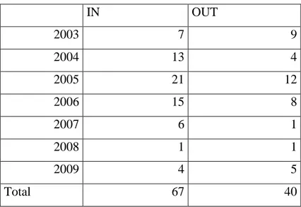
Now it is time to articulate the content of this thesis. In the first chapter, I introduce the concept of Capital Market Theories, in particular the concept and the main characteristics of Efficient Market Theory (EHM) and The Capital Asset Pricing Model (CAPM). In the second chapter generally is spoken about empirical studies regarding market efficiencies and index variation. Particularly, the main idea of the second chapter is to point out why neither EMH, nor CAPM cannot explain the event of abnormal returns due to a stock’s inclusion/exclusion from an index. That is for two main reasons: 1) some stock market anomalies have been shown to be quite robust to violate the efficient market hypothesis while supporters of the efficient market hypothesis can argue that many of the violations of the hypothesis (subsequently explained) are instead examples of the ‘bad model’ problem related to the simplifying assumption of the CAPM. In the third chapter is shown the main object of this thesis and the methodology used (The Event-Study Methodology). In practice, event studies have been used for two major reasons: 1) to test the null hypothesis that the market efficiently incorporates new information and 2) under the hypothesis of market efficiency, to examine the impact of some event on the wealth of the firm’s security holders. After having explained the methodology, this thesis is dedicated to the sample description either for S&P/MIB, FTSE MIB or Midex and FTSE Italia Mid Cap. For S&P/Mib there were 34 changes (17 stocks IN and 17 stocks OUT) while for FTSE Mib there were just 14 (7 stocks IN and 7 stocks OUT). We consider interesting to extend this study also for the case of Midex (67 stocks IN and 40 stocks OUT) and Ftse Italia Mid Cap (39 stocks IN and 38 stocks OUT) especially for the analysis of trading
volumes as for the stock with a lower level of capitalization the effect of abnormal trading volume could be more evident. To conclude in this chapter a part is dedicated to the result interpretation and the final conclusions.
However, it is important to point out the limits of this study. The small number of observation, especially for the S&P/Mib and FTSE Mib could determine statistically non - significant results. the fact the addition/deletion from the index may happen at some “particular” moment of a firm’s life, so the price effect may be related to index rebalancing or to other causes, which make it more difficult to reasonably
Chapter 1- Capital market theories
1. The foundation of modern capital market theories
Capital market theories provide the foundation for the development of financial asset pricing models. The principal view of capital markets adopt the ‘’perfect-world’’ scenario where markets are perfectly efficient and the asset prices quickly and accurately reflect all the new information available in the market. Under the assumption of efficient capital markets, all the investors are risk-averse and completely rational in making their decisions. Theories developed based on the assumption of efficient capital markets include Markowitz’s portfolio theory, the separation theorem, the Capital Asset Pricing Model (CAPM) and the arbitrage pricing theory (APT).
The efficient market hypothesis (EMH), postulates that asset prices fully reflect all relevant information, and the implications of this theory are that stock prices are not predictable and investors cannot earn abnormal returns. Modern Portfolio Theory (MPT), developed by Markowitz (1952) and the separation theorem of Tobin (1958) provide solutions for risk-averse investors to allocate assets in an efficient capital market. Under the assumptions of MPT, risk-averse investors have homogeneous expectations regarding the mean, variance, and covariance of asset returns, and aim to maximize their expected utility when making investment decisions. As an extension of MPT, the capital asset pricing model (CAPM) is developed to determine the price of assets in an efficient capital market.
1.1 Efficient Market Hypothesis (EHM)
The concept of Efficient Market Hypothesis was first introduced by Fama in the 1969. An ‘efficient market’ was defined as a market which ‘adjusts rapidly to new information’ and correctly evaluate the available information.
However, it is clear that while rapid adjustment to new information is an important element of an efficient market, it is not the only one. A more modern definition is that asset prices in an efficient market ‘fully reflect all available information’ (Fama 1991). This implies that the market processes information rationally, in the sense that relevant information is not ignored, and systematic errors are not made. As a consequence, prices are always at levels consistent with ‘fundamentals’. This is a strong version of the hypothesis that could only be literally true if ‘all available information’ was costless. If
information was instead costly, there must be a financial incentive to obtain it. But there would not be a financial incentive if the information was already ‘fully reflected’ in asset prices (Grossman and Stiglitz 1980).
A weaker, but economically more realistic, version of the hypothesis is therefore that prices reflect information up to the point where the marginal benefits of using the information (the expected profits to be made) do not exceed the marginal costs of collecting it (Jensen 1978). Secondly, what does it mean to say that prices are consistent with fundamentals?
We must have a model to provide a link from economic fundamentals to asset prices. While there are candidate models in all asset markets, no-one is confident that these models fully capture the link in an empirically convincing way. This is important since empirical tests of market efficiency, especially those that examine asset returns over extended periods of time, are necessarily joint tests of market efficiency and a particular asset-priceing model. When the joint hypothesis is rejected, as it often is, it is logically possible that this is a consequence of deficiencies in the particular model rather than market inefficiency . This is the ‘bad model’ problem (Fama 1991)i.
Finally, market efficiency means serval “positive things”. Not only the fact of reflecting all the available information, but also the concept of efficiency in resource allocation. However in this thesis we are concentrating in the informative efficiency. The role of an efficient market is not only reflect available information (at least up to the point consistent with the cost of collecting the information) but also guarantee efficient resource allocation.
1.1.1 The Three Forms of Market Efficiency
Three assumptions hold for a market to be efficient:
1) A large number of competing profit-maximizing participants independently of each other analyze and value securities;
2) new information regarding securities comes to the market in a random way 3) and the fact that investors are rational (they want to maximize their profits). In economic and financial theory a distinction is made between three forms of market efficiency. The basis of this separation is what is meant by the term “all available information”.
The EMH has historically been subdivided into three categories (Robert (1967)):
a) The weak form of Efficient Market Hypothesis (EMH) assumes that the price of a share at any time fully reflects all the market information of that security such as its past prices, returns, and trading volumes. This hypothesis implies that these past returns should have no connection with the future ones. So, future rates of the return should be independent. That implies that investors should not gain from any trading rule that decides when to buy or sell a security based only on the information of its past rates of return or past market prices. If weak-form efficiency holds, stock prices should be composed only of three components – the last period’s price, the expected return on the stock and a random error term which has an expected value of zero. This random error is due to new, unexpected information released in the period observed. Their relationship can be expressed as follows:
Pt = Pt-1+E(r) +Є (1) Where Pt is the stock price in period t, E(r) is the expected return on the stock, and Є is random error term.
b) The semi-strong form efficient market hypothesis (EHM) implies that a share price reflects all the publicly available information. Additionally to the market information, the public information includes all non-market information such as earnings and dividend announcements, price-to-earnings (P/E), book value-market value (BV/MV), and other ratios. The semi-strong EMH implies that investors, who adjust their decisions with new information, should not abnormal returns since in a such market all the prices of securities already reflect all that publicly available information.
c) Strong form EMH assumes that stock prices reflect all public and private information. This means that no group of investors has access to some information relevant to the stock, so no group of investors should be able to make above-average returns even if this piece of information is not publicly available. The point here is that it allows to aggregate the new information into the prices and this is just a theoretical form of efficiency (e.g. this implies a null profit for the insiders)
1.2 Event Studies and Market Efficiency
A number of studies1 have suggested that there exists a high level of efficiency in capital markets. If this suggestion is true, then one would expect that security prices would reflect available information. Thus, the “purchase or sale of any security at the prevailing market price represents a zero NPV transaction.”
One should be able to determine the relevance of a given type of information by examining the effect of its occurrence on security prices. Thus, non-random performance of security prices immediately after a given event suggests that news of the event has a significant effect on security values. The degree of efficiency in a market to a given type of information may be reflected in the speed that the market reacts to the new information. The impact of the event on security prices is typically measured as a function of the amount of time that occurs between the event and stock price change. In a efficient market, one might expect that the effect of the event on security prices will occur very quickly, so event studies are usually based on daily, hourly or even trade to trade stock price fluctuations. For example, analysts are often able to predict with a reasonably high degree of accuracy firm earnings and trade securities on the basis of their predictions. Thus the impact of corporate earnings changes may be realized in security price long before earnings reports are officially released. Thus, one may need to study the impact of a given event, news item or announcement by considering security price reactions even before the event occurs. In these case the event study should focus on the new information, the one that the market does not expect (e.g. in the case of earnings, it is often said “surprise earnings” a higher or lower result regarding the analyst’s expectation. The main concern here is to define exactly the moment when the news is released.
So, an event study is concerned with the impact of a specific type of new information of a security's price. Given that more than one piece of news may be affecting the security's price at any given point in time, one will probably need to study more than one firm in order to have statistically a greater opportunity to refuse H0 , given that, as
the sample size reduces the variability of the estimator. Thus, a population or sampling of firms experiencing the given event will be gathered, and the impact of the event on each of the firms' securities will be studied simultaneously. If a sufficiently large
1 Brown, Stephen J. and Jerold B. Warner, "Measuring Security Price Performance," Journal of Financial Economics”.
number of firms experiencing the event are sampled randomly, then the single commonality among the firms is the event2.
2. Asset pricing in an efficient capital market – The Capital Asset Pricing Model A substantial part of the research effort in finance is directed toward improving our understanding of how investors value risky cash flows. It is generally agreed that investors demand a higher expected return for investing in riskier projects, or securities. However, we still do not fully understand how investors assess the risk of a project's cash flow and how they determine what risk premium to demand.
Serval capital asset pricing models have been suggested in the literature. Among them, Sharpe – Lintner3 model Capital Asset Pricing Model is the one that financial managers most often use for assessing the risk of the cash flows from a project and arriving at the appropriate discount rate to use in valuing the project. According to the CAPM, (a) the risk of a project is measured by the beta of the cash flows with respect to the return on the market portfolio composed by all assets in the economy, and (b) the relation between required expected return and beta is linear.
2.1 Assumptions of the CAPM
The assumptions of CAPM can be divided into three sets of conditions: (1) the markets are in equilibrium; (2) that all investors behave according to a mean-variance criterion; and (3) that investors have the same expectations regarding the mean, variances and covariances – the investors are said to have homogeneous beliefs.
1: Asset market characteristics
2
A nonzero correlation in the sample would indicate that abnormal return is systematically related to information revealed in the event (i.e., there exists an information effect). Conversely, zero correlation implies lack of an information effect. “Conditional Methods in Event Studies and an Equilibrium Justification for Standard Event-Study Procedures”. N. R. Prabhala, Yale University.
3
The capital asset pricing model (CAPM) of William Sharpe (1964) and John Lintner (1965) marks the birth of asset pricing theory (resulting in a Nobel Prize for Sharpe in (1990)).
a. Frictionless market. This assumptions has two elements: 1) zero transaction costs; 2) no institutional restrictions on asset trades (e.g. short sales are allowed). This assumptions is an idealization because hardly ever it is satisfied in practice.
b. Investors can borrow or lend unlimited amounts at the risk- free rate of interest. Such an assumption is clearly not descriptive of the real world. It seems much more realistic to assume that investors can lend unlimited sums of money at the riskless rate but cannot borrow at a riskless rate. Furthermore it is not possible for investors to borrow unlimited amount at a riskless rate.
c. Asset are perfectly divisible into smaller units.
d. All assets can be bought or sold at observed market prices.
e. Investors are price-takers: the decision of any investor do not affect asset prices. f. Taxes are neutral. What is relevant for the following analysis is not the common
assumption that taxes are zero, but the fact that all investors face the same the same tax rates.
2 : Mean-variance portfolio selection
a. All investors behave according to a single-period investment horizon. Hence, their objectives focus on the terminal value at a specified date in the future.
3: Homogeneous beliefs
a. All investors use the same estimates of the expectations, variances and covariances of assets returns.
The Capital Asset Pricing Model (CAPM) describes the relation among the expected return of a given asset i, denoted by E(ri), the risk-free return offered by the economy,
Rf, the return offered by the market portfolio RM and one risk measure of the asset being
discussed, called beta coefficient, represented by β. The equation below specifies the relation proposed by the CAPM model:
E(ri)= Rf + βi (RM-Rf) (2)
One of the most important points to be considered in this model is the return of the market portfolio, which can be defined as a portfolio containing investments in all the financial assets, corresponding to the market value of each asset considered. This portfolio is a theoretical abstraction that, if taken to the real world, is approximated by
an index containing the listed assets. The CAPM conveys the notion that securities are priced so that the expected returns will compensate investors for the expected risks. There are two fundamental relationships: the capital market line and the security market line. The capital market line specifies the return individual investors expect to receive on a portfolio. The security market line expresses the equilibrium return an individual investor can expect. The model predicts that expected return on a stock above the risk free rate has linear relation with non-diversifiable risk as measured by stocks’ beta.
2.2 The Fama and French three-factors model
Capital Asset Pricing Model (CAPM) considers the relationship between expected return of an asset and it’s systematic risk, measured by beta (β). In order to avoid CAPMs’ limitations a more complicated model is used to measure assets return, the Fama and French three-factors model.
The Fama and French model (1992) was enriched, after some papers proposed by Carhart, with the momentum factor, so recently the model is specified as follows:
Ri – Rf = α + bm (Rm - Rf) + bs SMB + bv HML+ wiWML +ui (3)
where variable definitions are as above:
a is the return when the factor portfolio returns are zero; the b’s are sensitivities to each source of risk;
SMB (Small Minus Big) is the average rate of return of the portfolio with small minus big portfolios;
HML (High Minus Low) is the average return of high value portfolios minus the average return of low value portfolios;
a momentum return, WML(t), the difference between the month t returns on diversified portfolios of the winners and losers of the past year;
Rm-Rf is the risk premium (the difference between the average market rate of return and the risk free rate);
The research of Fama and French (1993) identified five risk factors affecting the rate of return of stocks and bonds. There were three market risks of the stocks: the general market factor, the factor related to size and a factor related to the book to market price (B/M). The two rest factors were belonged to the bond market: the term factor and the risk of default. It is important to note that there was a significant relationship between these five factors and the rate of return of the stocks and bonds. In the market, the change in profit in the short term had affected the stock price and the BE/ME ratio. The relationship between BE/ME with the profit differences is only significant in the long-term. Those companies had the high BE/ME ratios (market price low relative to book value) tend to prolong the recession. By contrast, the ones with low BE/ME ratios (market price high relative to book value tend to maintain strongly profitability. Like all asset pricing models, however, the CAPM and the Fama and French model are incomplete descriptions of average returns4.
3 The liquidity premium
The role of liquidity in empirical finance has grown rapidly over the past fifty years influencing conclusions in asset pricing, market efficiency and corporate finance. A number of studies5 have proposed liquidity measures derived from daily return and volume data as proxies for investors’ liquidity and transaction costs. Liquidity is concept that generally denotes the ability to trade large quantities quickly, at low cost,
4
Ravi Jagannathan and Zhenyu Wang:” The CAPM is Alive and Well”. In this paper they argue that the incompleteness of the CAPM are well known due to the perfect market assumption, the difficulties of choosing the representative portfolio, values need to be assigned to the risk-free rate of return, the return on the market or the equity risk premium (ERP). Fama and French (1993) show that their three-factor model does not even provide a full explanation of average returns on portfolios formed on size and BE/ME, the dimensions of average returns that the models risk factors are designed to explain.
5 Ruslan Y. Goyenkoa, Craig W. Holdenb, Charles A. Trzcinka (2008), “Do liquidity measures
measure liquidity”? Commonality in liquidity; Tarun Chordia, Richard Roll e Avanidhar Subrahmanyam, (2000), Journal of financial economics. Liquidity and market efficiency, Chordia, Roll e Subrahmanyam, Journal of Financial Economics, (2008).
and without moving the price. The relation between expected stock returns and liquidity has been investigated by numerous empirical studies, from the seminal papers of Amihud and Mendelson (1986) and Brennan and Subrahmanyam (1996). Using a variety of liquidity measures, these studies generally found that less liquid stocks have higher average returns, which in turn benefit investors with long trading horizons. Amihud and Mendelson showed that, in equilibrium, illiquid assets would be held by investors with longer investment horizons. As a result of this horizon clientele, they argued that the observed asset returns must be an increasing and concave function of the transactions costs. Using the bid–ask spread as a measure of liquidity, they tested the relationship between stock returns and liquidity during the period of 1961–1980, finding evidence consistent with the notion of liquidity premium. Eleswarapu and Reinganum (1993) propose a new proxy for liquidity because the bid-ask spread measure is two-fold. First, the data on bid–ask spread is hard to obtain on a monthly basis over long periods of time (A&M and E&R use the average of the bid–ask spread at the beginning and at the end of the year as a proxy for the liquidity of a stock through that year). Second, Peterson and Fialkowski (1994) show that the quoted spread is a poor proxy for the actual transactions costs faced by investors and call for an alternative proxy which may do a better job of capturing the liquidity of an asset.
Hence, another measure of liquidity is proposed in the financial literature: the turnover rate of an asset as a proxy for its liquidity. We define the turnover rate of a stock as the number of shares traded divided by the number of shares outstanding in that stock and think of it as an intuitive metric of the liquidity of the stock. The advantage of using the turnover rate as a proxy for liquidity are: first, it has strong theoretical appeal, since A&M proved that in equilibrium liquidity is correlated with trading frequency. So, if one cannot observe liquidity directly, the turnover rate can be used as a proxy for liquidity. Second, the data on turnover rates is relatively easy to obtain. This enables us to capture month by month variation in the liquidity of assets and allows the examination of liquidity effects across a large number of stocks over a long period of time.
An example of a contribution to support the hypothesis of liquidity is instead provided by Beneish and Gardner (1995), who focus their attention on the Dow Jones Industrial Average (DJIA), an index created in 1884 and composed of the 30 stocks selected among those "most actively traded and that are representative of the U.S. market". The changes in the index are determined by the editors of the Wall Street Journal without any external consultation. In fact, in the early ‘90s, the index was composed of stocks that weighed about 25% of the total capitalization of listed in the NYSE. This study also
point out how that the stocks chosen to be part of the index are usually the ones most actively traded in the market, while the stocks delisted from the index are often characterized by a modest capitalization and less traded in the market. This is in part to explain the results of the empirical investigation. If, in fact, for the securities being part of the index, there was no impact either on prices or volumes treated, we cannot say the same thing for the stocks excluded from the index. In the three days around the announcement date of the delisting, in fact, they observed a statistically significant negative abnormal return associated with a significant decrease in volumes handled. The asymmetric behavior of the two categories of the stocks traded is related to the explanation based on the liquidity and the cost of information. The stocks excluded from the index, apart from the fact that are traded less frequently in the market and less appealing to the investors, after the deletions they become less followed from the market and investors demand a premium for the higher transaction costs and the higher risk associated with the higher scarcity of information. In addition to the explanations related to the information component of liquidity, there are also those that refer to the so-called inventory theory, which is always referring to liquidity as the origin of the observed phenomena, as well proposing alternative explanations, largely related to transaction costs in case of liquidation. And 'well-known fact that investors require higher expected returns in the presence of a high bid-ask6 spreads, as they have to cover the cost of a more difficult disposal of their investment.
According to Amihud and Mendelson (1986), it can be argued that, if the securities are not maintained for an infinite time, the transaction costs are a constant flow to investor. If such cost increases as a result of delisting, the expected total cost of transaction grows significantly. The equilibrium model proposed by these authors calculates the gross yield as an increasing and concave function of the market liquidity. The proxy used to measure the degree of liquidity is the bid-ask spread and the proposed model of the expected return for the investor on asset j is:
E(Rij)Ri*iSj
6The amount by which the ask price exceeds the bid. This is essentially the difference in price
between the highest price that a buyer is willing to pay for an asset and the lowest price for which a seller is willing to see.
Where the equilibrium return in a perfectly liquid market (Ri*), is corrected by a factor µiSj which is the expected cost of the liquidation (calculated as the product of the probability of liquidation µi and the spread of the good considered Sj. If after the listing
the spreads decrease, the lower return required by investors will lead to an increase in the stock’s value.
It is easy to see how the empirical evidence of the validity of the liquidity hypothesis takes into account the joint observation of spreads and trading volumes. If the first decrease and the second increase when the event is announced (and in subsequent periods), then one can speak of a real effect on the liquidity of the securities concerned.
Chapter 2 - Empirical studies regarding market efficiencies
and index variation
1.The Predictions of the Efficient Market Hypothesis
The available evidence suggests that financial market returns are partly predictable, in ways that sometimes conflict with the efficient market hypothesis. There have been several responses to this evidence. Many stock market anomalies may be due to ‘data-snooping’7
(Lo and MacKinlay 1990). Fama (1998) makes the related point that many anomalies are sensitive to the research methodology used, and disappear when reasonable changes in technique are applied. Nevertheless, other stock market anomalies – for example, post-earnings-announcement drift – have been shown to be quite robust. It should also be noted that the extent of predictability observed in the data is never high. Whether for stocks, exchange rates or fixed-interest securities, and whether at short or long horizons, most of the variation in prices is unexpected. The small degree of predictability that is present may not be large or stable enough to provide the basis for a trading strategy capable of generating economic profits once transaction costs are taken into account. This may explain why market participants do not ‘trade away’ the observed predictability in asset returns. However, it does not explain why such predictability exists in the first place.
Finally, observed predictability in returns may reflect variation over time in the size of the risk premium (Bollerslev and Hodrick 1992). This premium is the ‘extra’ return that investors require over and above the risk-free rate to compensate them for investing in a risky asset. However, as Hodrick (1990) and Lewis (1995) acknowledge, we have no satisfactory models of risk premium in either the stock market or the foreign exchange
7
"Data snooping occurs when a given set of data is used more than once for purposes of inference or model selection. When such data reuse occurs, there is always the possibility that any satisfactory results obtained may simply be due to chance rather than to any merit inherent in the method yielding the results. This problem is practically unavoidable in the analysis of time-series data, as typically only a single history measuring a given phenomenon of interest is available for analysis.
market. Whatever the correct model of risk premium, market agents must be extraordinarily risk-averse for the data on asset returns to be consistent with the efficient market hypothesis (Mehra and Prescott 1985; Hansen and Jagannathan 1991). To conclude, we can always explain predictability in asset returns as reflecting changes in unobservable risk. But such an explanation is, as it stands, empirically empty.
Do Asset Prices Move as Random Walks?
Asset prices in an efficient market should fluctuate randomly through time in response to the unanticipated component of news (Samuelson 1965). Prices may exhibit trends over time, in order that the total return on a financial asset exceeds the return on a risk-free asset by an amount related to its risk. Fluctuations in the asset price away from trend should be unpredictable, however, the evidence suggests that that the hypothesis of random walk is at least approximately true. While stock returns are partially predictable, both in the short run and the long run, the degree of predictability is generally small compared to the high variability of returns. In the aggregate US sharemarket, above-average stock returns over a daily, weekly or monthly interval increase the likelihood of further above-average returns in the subsequent period (Campbell, Lo and MacKinlay 1997). However, for example, only about 12 per cent of the variance in the daily stock price index can be predicted using the previous day’s return. Portfolios of small stocks display a greater degree of predictability than portfolios of large stocks. There is also some weak evidence that the degree of predictability has diminished over time.
In a related literature, a number of studies have found evidence of mean reversion in returns on stock portfolios at horizons of three to five years or longer (Poterba and Summers 1988; Fama and French 1988). This implies that a long period of below-average stock returns increases the likelihood of a period of above-below-average returns in the future. These conclusions are less robust, however, than the findings of short-run predictability in returns. The most important problem is that since long-horizon returns are measured over years, rather than days or weeks, there are far fewer data points available, making precise statistical inference difficult. For example, Poterba and Summers are unable to reject (in a statistical sense) the null hypothesis of no serial correlation in returns, even though their point estimates suggest a substantial degree of returns predictability, and despite their use of a span of sixty years of data.
Is New Information Quickly Incorporated into Asset Prices?
The efficient market hypothesis explain that stock prices respond quickly to new information, and subsequently show no apparent strong trends. Event studies, pioneered by Fama (1969), generally found that price adjustment is due to the following major events such as mergers, stock-splits or changes in firms’ dividend policies. Despite this general finding of rapidly adjusting stock prices, some puzzling results remain. Most notable among these is the fact that stock prices do not adjust instantaneously to profit announcements. Instead, on average a firm’s share price continues to rise (fall) for a substantial period after the announcement of an unexpectedly high (low) profit. This anomaly appears to be quite robust to changes in sample period.
Can Current Information Predict Future Excess Returns?
In an efficient market, publicly available information should already be reflected in the asset price. In the stock market, for example, public information on price-earnings ratios, cash flows or other measures of value should not have implications for future share returns (unless these variables are revealing information about the riskiness of the asset). The history of asset prices should also have no predictive power for future asset returns.
Empirical evidence shows that neither Efficient Market Hypothesis nor CAPM cannot explain the actual movements of asset returns. The first step to made is to see why the EMH cannot explain the asset returns. The efficient market hypothesis provide a number of interesting and testable predictions about the behavior of financial asset prices and returns. One of them is market inefficiencies and behavioral finance.
1.1 Market Inefficiencies
In this section, I discuss stock market anomalies – public information about stocks which helps to predict excess returns. I begin with a selection of stock market anomalies:
Value effects
Portfolios constructed from ‘value’ stocks appear to produce superior investment returns over long horizons. Value stocks are those with high earnings, cash flows, or tangible assets relative to the current share price. After controlling for firm size and the
variance of portfolio returns, stocks with low price-earnings ratios outperform the market (Fama and French 1992). Also, portfolios of stocks with poor past returns produce higher returns than the market as a whole over subsequent periods. De Bondt and Thaler (1985) 8construct portfolios ordered across various measures of value, such as book-to-market, cash-flow-to-price and price-earnings ratios, sales growth and past returns history, using historical data on US stock returns. Along each of these dimensions, portfolios constructed from value stocks exhibit high future returns relative to ‘high performance’ portfolios over investment horizons of between one and five years. Lakonishok, Shleifer and Vishny (1994) found similar findings, and also present evidence that the variability of returns from value portfolios is no greater than for “high performance” portfolios. Thus, the higher returns earned by value portfolios do not appear to be due to a higher level of risk.
Momentum effects
Although value stocks produce superior returns over long investment horizons, in the short run the opposite seems to hold. Jegadeesh and Titman (1993) find that portfolios with high returns in the recent past continue to produce above-average returns over a 3−12 month horizon. Chan, Jegadeesh and Lakonishok (1996) provide evidence that this ‘momentum’ in stock returns can be partially accounted for by the slow adjustment of the market to past profit surprises.
Size anomalies
Small firms’ stocks exhibit higher average returns (Banz 1981) although this may reflect a distressed-firm effect (Chan and Chen 1991). Since small firms include a disproportionate number of companies in financial distress, the higher expected returns experienced by small stocks may be a compensation for exposure to the risks associated with these distressed firms. While there is some relationship between these anomalies, they do appear to be distinct phenomena. For example, small firms generally have lower
8
An alternative behavioral explanation for the anomaly based on investor overreaction is what Bsau called ‘’price-ratio’’ ratio hypothesis. Companies with very low P/E ratio are thought to be ‘’undervalued’’ because investors become excessively pessimistic after a series of bad earnings reports or other bad news. Once future earnings turn out to be better than furcating, the price adjusts. Similarly, the equity of companies with very high P/E ratio, is thought to be ‘’overvalued ‘’ before falling in price.
price-earnings ratios and relatively poor past earnings growth (Chan, Hamao and Lakonishok 1991) and thus are more likely to be classified as value stocks.
They find that when stocks are ranked on three- to five-year past returns, past winners tend to be future losers, and vice versa. They attribute these long-term return reversals to investor overreaction. In forming expectations, investors give too much weight to the past performance of firms and too little to the fact that performance tends to mean-revert. DeBondt and Thaler seem to argue that overreaction to past information is a general prediction of the behavioral decision theory of Tversky and Kahneman. Thus, one could take overreaction to be the prediction of a behavioral finance alternative to market efficiency.
Other studies also produce long-term post-event abnormal returns that suggest underreaction. Cusatis (1993) find positive post-event abnormal returns for divesting firms and the firms they divest. They attribute the result to market underreaction to an enhanced probability that, after a spinoff, both the parent and the spinoff are likely to become merger targets, and the receivers of premiums. Ikenberry (1996) find that firms that split their stock, experience long-term positive abnormal returns both before and after the split. They attribute the post-split returns to market underreaction to the positive information signaled by a split. Lakonshik and Vreamlen (1990) find positive long-term post-event abnormal returns when firms tender for their stock. Ikenberry (1996) observe similar results for open-market share repurchases. The story in both cases is that the market under-reacts to the positive signal in share repurchases about future performance.
Some long-term return anomalies are difficult to classify. For example, Asquith (1983) find negative long-term abnormal returns to acquiring firms following mergers. This might be attributed to market underreaction to a poor investment decision (Roll, 1986) or overreaction to the typically strong performance of acquiring firms in advance of mergers. Ikenberry and Lakonishok (1993) find negative post-event abnormal returns for firms involved in proxy contests. One story is that stock prices under-react to the poor performance of these firms before the proxy contest, but another is that prices over-react to the information in a proxy that something is likely to change.
1.2 Behavioral Finance
In the 1990’s lot of the focus of academic discussion shifted away from the econometric analyses of time series on prices, dividends and earnings, towards developing models of human psychology as it relates to financial markets. Behavioral finance attempts to explain the emotional processes involved and the degree to which they influence the decision-making process. Essentially, behavioral finance attempts to explain the what, why, and how of finance and investing, from a human perspective. For instance, behavioral finance studies financial markets as well as providing explanations to many stock market anomalies, speculative market bubbles, and crashes. Behavioral finance studies the psychological and sociological factors that influence the financial decision making process.
Some of the factors that influence the financial decision making process are:
Overconfidence: According to Ricciardi and Simon (2000), human beings have the tendency to overestimate their own skills and predictions for success, or an overestimation of the probabilities for a set of events. Overconfidence manifests itself in a number of ways. One example is e is too little diversification, because of a tendency to invest too much in what one is familiar with.
Framing: Frames are a part of Tversky and Kahneman’s prospect theory 9. Prospect theory deals with the idea that people do not always behave rationally. Frame dependence manifests itself in the way people form attitudes towards gains and losses. Many people make one decision if a problem is framed in terms of losses, but behave differently if the same problem is framed in terms of gains. An important reason for this behavior is loss-aversion. Loss-aversion refers to the tendency for decision makers to weigh losses more heavily than gains; losses hurt roughly twice as much as gains feel good.
9
Daniel Kahneman e Amos Tversky, Prospect Theory: An Analysis of Decision Under Risk (1979). The effect of frames on preferences are compared to the effect of perspectives on perceptual appearance. The dependence of preferences on the formulation of decision problems is a significant concern for the theory of prospect.
Mental Accounting: People often keep their portfolio money in separate mental accounts or ‘pockets’. They behave this way to protect their accounts from downside risk etc.
2. The Fama and French Empirical Study Regarding The CAPM’s Invalidity The second step is to show evidence why Capital Asset Pricing Model cannot explain the assets returns. Over the past two decades a number of studies have empirically examined the validity of the CAPM. The results reported in these studies support the view that it is possible to construct a set of portfolio such that the CAPM has little ability to explain the cross sectional variation in average returns among them. In particular, portfolio containing stocks with relatively small capitalization appear to earn positive excess returns on average than those predicted by the CAPM. In spite of the lack of empirical support, the CAPM is still the preferred model for pricing the assets. Hence, the CAPM still ‘survives’ because: (a) empirical support for other asset pricing models is no better, (b) the theory behind the CAPM has an intuitive appeal that is hard to beat using the other models, and (c) the economic importance of the empirical evidence against the CAPM reported in empirical studies is ambiguous.
Nevertheless its success in their study, Fama and French (1992) present evidence suggesting that the statistical rejections of the CAPM that have been reported in the literature may also be economically important. They examined the CAPM using return data on a large collection of assets and found that the relation between market β and average return is flat and the relation between average return and size is negative. Fama and French point out the robustness of the size effect and the absence of a relation between β and average return that are so contrary to the CAPM.
2.1 The Bad Model
One of the explanation of the CAPM’s invalidity is due to ‘Bad Model’. Bad-model problems are of two types. First, any asset pricing model is just a model and so does not completely describe expected returns. For example, the CAPM of Sharpe (1964) and Lintner (1965) does not seem to describe expected returns on small stocks. Second,
even if there were a true model, any sample period produces systematic deviations from the models predictions, that is, sample-specific patterns in average returns that are due to chance. For example, empirical studies evidence that small stocks have higher average returns than predicted by the CAPM, an event stock’s abnormal return is often estimated as the difference between its return and the return on non-event stocks matched to the event stock on size. Following the evidence of Fama and French (1992) that average stock returns are also related to book-to-market equity (BE/ME), it is now common to estimate abnormal returns by matching event stocks with non-event stocks similar in terms of size and BE/ME. When we analyze individual event studies, we shall see that matching on size can produce much different abnormal returns than matching on size and BE/ME. Both size and BE/ME surely do not capture all relevant cross-firm variation in average returns due to expected returns or sample-specific patterns in average returns. One approach to limiting bad-model problems may be by using firm-specific models for expected returns. For example, the stock split study of Fama (1969) uses the market model to measure abnormal returns.
Another method of estimating abnormal returns is to use the three-factor model of Fama and French (1993). Like all asset pricing models, however, the CAPM and the Fama and French model are incomplete descriptions of average returns. Fama and French (1993) show that their three-factor model does not even provide a full explanation of average returns on portfolios formed on size and BE/ME, the dimensions of average returns that the model’s risk factors are designed to capture. In short, bad-model problems are unavoidable, and they are more serious in tests on long-term returns.
2.2 Consequences
The introduction of the efficient market hypothesis thirty years ago was a major intellectual advance. The hypothesis provided a powerful analytical framework for understanding asset prices.
Nevertheless, despite its successes, other features of asset-market behavior seem much harder to reconcile with the efficient market hypothesis. Some stock market anomalies have been shown to be quite robust to violate the efficient market hypothesis. Supporters of the efficient market hypothesis can argue that many of the violations of
the hypothesis (above explained) are instead examples of the ‘bad model’ problem. Under this interpretation, predictable excess returns represent compensation for risk, which is incorrectly measured by the asset-pricing model being used.
3.The hypotheses that explain the index effect
In these section are explained the hypotheses that justify the performance of stocks’ returns and trading volume during the event window.
Neither efficient market hypothesis (EMH) nor CAPM, cannot explain the abnormal returns and trading volumes for the following reasons:(1) Market inefficiencies can affect not only average returns but also return covariances, and this problem is likely to be more severe the higher the frequency of the returns. (2) Regarding the ability of the CAPM to explain value and growth stocks’ price levels, the empirical results suggest that mispricing relative to the CAPM is not necessarily an important factor in determining the price levels of value and growth stocks.
The index effect has been shown in numerous other studies and result in unusual stock price and excessive trading volume during the event period that it is not consistent with the efficient market hypothesis (EHM) or capital asset pricing model (CAPM). Consequently, a number of hypothesis have been considered to justify this performance. The following hypothesis regards S&P 500 index, but they can also be applied in the case of these study. The hypothesis that have been proposed in the literature are: the Price Pressure Hypothesis, the Imperfect Substitutes/Downward Sloping Demand Curve for Stock Hypothesis, the Liquidity Cost Hypothesis, the Information Content/Index Member Certification Hypothesis, and the Market Segmentation/Investor Recognition Hypothesis. Their main differences concern whether the stock price or volume change is temporary or permanent after the event, what kind of information is revealed with an addition or deletion, and what are the main issues for investor behavior.
3.1 The Price Pressure Hypothesis (PPH)
The concept of this hypothesis is that investors who provide liquidity to the market without having any motivation to trade should be compensated by a premium that
reflects their extra costs and the risk of these trades. Harris and Gurel’s (1986)10
results were in favor of the Price Pressure Hypothesis since they found a significant stock price increase of 3.13% after inclusion, which was fully reversed after two weeks. Regarding the trading volumes, they also increased temporarily for the period around the event. Arnott and Vincent (1986) found price increases for additions and price decreases for deletions and both were significant and persistent for a period of four weeks after the event.
Regarding the Italian Stock Exchange, the price pressure hypothesis explains that the price increase is due to the buying activity of index funds. So prices increase temporarily in order to induce passive investor to supply the stocks to index funds. This hypothesis also states that change in demand (supply) is only temporary during the announcement date or effective date when investors are rebalancing their portfolios. Such short-term imbalances can cause a temporary stock price effect. Hence the price will temporary increase by the excess demand for funds included in the index following the announcement date and will revert to the original equilibrium after the event window.
3.2 The Imperfect Substitutes and the Downward-Sloping Demand Curve for Stocks Hypothesis
The imperfect substitutes hypothesis holds that stocks belonging to the S&P 500 Index do not have perfect substitutes and have downward-sloping demand curves (Scholes 1972). According to this hypothesis, prices will change to eliminate any excess demand in the market and no reversal is expected in the long-term.
In the Downward-Sloping Demand Curve for Stocks Hypothesis, abnormal trading activity should be temporary until the new level of price equilibrium is reached. The DSH was first proposed by Shleifer (1986) and it contrasts the Price Pressure Hypothesis. While the PPH assumes a downward-sloping curve in the short run, the DSH assumes a downward-sloping curve in both short run and in the long-run. This
10
Harris and Gurel studied the price and volume effect associated with changes in the S&P 500 list (1986). New evidence for the existence of Price Pressure Hypothesis. Their results are consistent with the price pressure hypothesis: immediately after an addition is announced, prices increase by 3% and reverse after two weeks.
hypothesis explain that the share price increases at the announcement date of an index addition due to the shift of the demand curve for stocks.
3.3 The Liquidity Cost Hypothesis (LCH)
Since the S&P 500 includes the majority of leading index funds, inclusion should enhance the liquidity of the added stock. Liquidity ensures the ability to sell a stock immediately and at an appropriate price.
Mikkelson and Partch (1985) found that an increase in the stock’s liquidity could result in an increase in its price due to lower transaction costs. According to the Liquidity Cost Hypothesis (LCH), inclusion in the index is an event that promises a permanent increase in the stock’s liquidity, and therefore both stock price and trading volume should see a permanent increase, rejecting the Pressure Hypothesis, as well as the Downward Sloping Demand Curve Hypothesis. Erwin and Miller (1998) were also in favor of the Liquidity Cost Hypothesis, since they observed a significant decrease in both the relative and absolute bid-ask spread when a stock was added to the S&P 500.
3.4 The Information Content Hypothesis and the Certification of an Index Member (ICH)
According to this hypothesis, when a stock is included in the index, an important piece of information is revealed that should have a permanent effect on prices and a temporary effect on volume. The S&P 500 certification effect can increase the firm’s expected future cash flows since inclusion will help companies to attract new capital more easily because financial institutions may be more willing to lend to firms that are index members. The Information Content Hypothesis was supported by the findings of Dhillon and Johnson (1991)8, who observed changes in stock prices, bond prices and option prices and found permanent effects. So, inclusion conveys new information concerning the investment appeal of a company and have a permanent effect on prices and a temporary effect on volume.
3.5 The Market- Segmentation and Investor Recognition Hypothesis (IRH) According to Merton’s (1987)11
Investor Recognition Hypothesis, investors have knowledge of only a subset of all stocks (in this case, only S&P 500 member stocks), hold only the stocks that they are aware of, and demand a premium (shadow cost) for the non-systematic risk that they bear. Hence, a stock’s inclusion in the S&P 500 Index alerts investors to its existence, and since this stock becomes part of their portfolios, the required rate of return should fall due to a reduction in non-systematic risk. According to Chen, Noronha and Singal’s observations (2002,2004) of cumulative abnormal returns, there was a permanent effect on the stock price after the index change, and the behavior of additions and deletions was not symmetrical, consistent with the Market Segmentation Hypothesis.
The Investor Awareness Hypothesis (IAH) states that if one stock enters into the index, investor awareness will be higher than before and many investors will more seriously consider buying it. This affects the shadow costs, which will be lower and the stock price will increase. However, if a company drops out of the index, the awareness of that company will not diminished immediately and shadow cost will not increase quickly.
11
Merton shows that, holding fundamentals constant, firm value is increasing in the degree of investor recognition of the firm. The key behavioral assumption invoked by Merton’s (1987) model is that investors only use securities that they know about in constructing their optimal portfolios.
Chapter 3 - An empirical evidence from changes in Italian indexes’ composition
1. The objectives of the analysis
This study examines the abnormal returns and trading volumes of stocks that were added to the most important Italian stock market indexes (S&P/Mib, FTSE Mib and FTSE Italia Mid Cap). The main objective of this analysis is to test whether the addition/deletion from the index has an impact on stock performance and liquidity. Regarding the Efficient Market Hypothesis (EMH), which postulates that asset prices fully reflect all relevant information, investors cannot earn abnormal returns and additions / deletions from the index: revisions should not have any impact on firm’s value, because index revision are mostly predictable at announcement dates and perfectly known at change dates. Of course, this fact stands as longs as the addition/deletion does not provide any new information to the market, otherwise the event should have an impact on stocks ‘prices and as a consequence on firm’s value. The index effect has been shown in numerous other studies to result in unusual stock price behavior during the event period that cannot be consistent with the efficient markets hypothesis (EMH) (see above). Consequently, a number of other hypotheses (previously mentioned) have been considered to justify this performance.
According to the Liquidity Cost Hypothesis (LCH), the inclusion in the index is an event that promises a permanent increase in the stock’s liquidity and therefore prices and trading volumes should both increase permanently to reflect the fact of being part of the index ( in this case part of the S&P/Mib, FTSE Mib or FTSE Italia Mid Cap). On the other hand, from the perspective of the Information Content Hypothesis (ICH), when a firm becomes a member of the index, this event conveys a meaningful piece of information such as improved or expected operating performance to investors.
According to the Investor Awareness Hypothesis (IAH), if one stock enters into the index, investor awareness of the stock will be higher than before and many investors will more seriously consider buying it. This affects the shadow cost which will be lower, and the stocks ‘price will increase. All these hypothesis explain that the inclusion on the index has a positive impact on stock’s performance.
In this study the empirical evidence regards changes in Italian indexes ‘composition. In order to verify the presence of abnormal returns due to changes in the index composition three indexes are taken into consideration, S&P/Mib, FTSE Mib and FTSE Italia Mid Cap (Midex).
From a temporal point of view, data cover approximately ten years, starting from year 2003 (year when S&P/Index was born) to year 2012. Regarding S&P/Mib and Midex the interval considered goes from year 2003 to June 2009 (the last year of their existence), rather for FTSE Mib and FTSE Italia Mid Cap it goes from September 2009 (year when they become operative) to 2012. In this elaboration a Return Index, adjusted for dividends and capital transaction, has been used to calculate returns (source is Datastream).
As it was mentioned before, the main objective of this analysis is to examine the impact of addition/deletion on the wealth of the firm’s security holders. In absence of abnormal returns during the period considered, CARs (Cumulative Abnormal Returns) should be not statistically significant.
2. The Event- Study Methodology
As it was mentioned in paragraph 1, Chapter 1, the Event-Study Methodology was first introduced by Fama, Fisher, Jensen and Roll (FFJR) (1969). FFJR started a methodological revolution in accounting and economics as well as finance, since the event study methodology has also been widely used in those disciplines to examine security price behavior around events such as accounting rule changes, earnings announcements, changes in the severity of regulation and money supply announcements.
The event study methodology has, in fact, become the standard tool for measuring security price reaction to some announcement or event. In practice, event studies have been used to test the null hypothesis that the market efficiently incorporates new information, examining the impact of some event on the wealth of the firm’s security
holders. For example, an event study might be conducted for the purpose of determining the impact of corporate earnings announcements on the stock price of the company. Many types of events are studied with event studies. Such events can include takeover announcements, environmental regulation enactments, patent filing announcements, competitor bankruptcy announcements, CEO resignation announcements, etc. Event studies are used to measure market efficiency, in other words, to determine whether prices respond immediately and correctly to the disclosure of new information. More important, from a trading perspective, event studies are used to back-test price data to determine the usefulness and reliability of trading strategies.
2.1 Steps in the Typical Event Study
Campbell, Lo and MacKinlay [1997] outline steps for the typical event study: 1. Define the event and establish the event window.
This means to establish exactly what the event is (e.g., the announcement of quarterly earnings for a firm) and determine the period during which security prices will be examined, in order to detect the effect of the event (this could be several seconds, minutes, hours, or days, but earlier studies were more likely to allow for months). The estimation window is typically the period prior to the event window, sometimes 120 days, but a “moving window” might include periods both before and after the event window. The event window must be separated from the estimation period so that parameters are not biased by the events.
Event studies are usually more effective when event windows are fairly short. Short-horizon event studies are relatively straightforward and trouble-free. This happens because Event-Studies focusing on announcement effects for a short-horizon around an event, allow to isolate the news from other events and this way to understand better the effects on firm’s value (performance). As well short-horizon test represent ‘‘the cleanest evidence we have on market efficiency’’ (Fama. 1991). Rather long-horizon methods present serious limitations. We know that inferences from long-horizon test require extreme caution and even using the best methods ‘‘the analysis of long-run abnormal returns is treacherous and unreliable’’(Lyon, Barber and Tsai, 1999). This is because in