Reverse Engineering tools: development and experimentation of innovative methods for physical and geometrical data integration and post-processing

(1)

A

l

m

a

M

a

t

e

r

S

t

u

d

i

o

r

u

m

–

U

n

i

v

e

r

s

i

t

à

d

i

B

o

l

o

g

n

a

DOTTORATO DI RICERCA IN

Meccanica e Scienze avanzate dell’Ingegneria:

Disegno e Metodi dell’Ingegneria Industriale e Scienze Aerospaziali

Ciclo XXV

Settore Concorsuale di afferenza: 09 / A3

Progettazione industriale, costruzioni meccaniche e metallurgia Settore Scientifico Disciplinare: ING / IND 15

Reverse Engineering tools: development and

experimentation of innovative methods for physical and

geometrical data integration and post-processing

Presentata da: Francesca Lucchi

Coordinatore Dottorato: Relatore:

Prof. Vincenzo Parenti Castelli Prof. Leonardo Seccia

Correlatori: Prof. Franco Persiani Ing. Francesca De Crescenzio

(2)

Alma Mater Studiorum – Università di Bologna Tesi di Dottorato

Francesca Lucchi

(3)

Abstract

In recent years, the use of Reverse Engineering systems has got a considerable interest for a wide number of applications. Therefore, many research activities are focused on accuracy and precision of the acquired data and post processing phase improvements. In this context, this PhD Thesis deals with the definition of two novel methods for data post processing and data fusion between physical and geometrical information.

In particular a technique has been defined for error definition in 3D points’ coordinates acquired by an optical triangulation laser scanner, with the aim to identify adequate correction arrays to apply under different acquisition parameters and operative conditions. Systematic error in data acquired is thus compensated, in order to increase accuracy value.

Moreover, the definition of a 3D thermogram is examined. Object geometrical information and its thermal properties, coming from a thermographic inspection, are combined in order to have a temperature value for each recognizable point. Data acquired by an optical triangulation laser scanner are also used to normalize temperature values and make thermal data independent from thermal-camera point of view.

Key words:

Reverse Engineering; Surface Accuracy; Measuring Uncertainties; Performances Evaluation; Metrological Characterization; Data Fusion; Thermography; 3D Thermography; Data Normalization.

(4)

(5)

Sommario

L’impiego di tecniche di Ingegneria Inversa si è ampiamente diffuso e consolidato negli ultimi anni, tanto che questi sistemi sono comunemente impiegati in numerose applicazioni. Pertanto, numerose attività di ricerca sono volte all’analisi del dato acquisito in termini di accuratezza e precisione ed alla definizione di tecniche innovative per il post processing. In questo panorama, l’attività di ricerca presentata in questa tesi di dottorato è rivolta alla definizione di due metodologie, l’una finalizzata a facilitare le operazioni di elaborazione del dato e l’altra a permettere un agevole data fusion tra informazioni fisiche e geometriche di uno stesso oggetto.

In particolare, il primo approccio prevede l’individuazione della componente di errore nelle coordinate di punti acquisiti mediate un sistema di scansione a triangolazione ottica. Un’opportuna matrice di correzione della componente sistematica è stata individuata, a seconda delle condizioni operative e dei parametri di acquisizione del sistema. Pertanto, si è raggiunto un miglioramento delle performance del sistema in termini di incremento dell’accuratezza del dato acquisito.

Il secondo tema di ricerca affrontato in questa tesi consiste nell’integrazione tra il dato geometrico proveniente da una scansione 3D e le informazioni sulla temperatura rilevata mediante un’indagine termografica. Si è così ottenuto un termogramma in 3D registrando opportunamente su ogni punto acquisito il relativo valore di temperatura. L’informazione geometrica, proveniente dalla scansione laser, è stata inoltre utilizzata per normalizzare il termogramma, rendendolo indipendente dal punto di vista della presa termografica.

(6)

(7)

List of Tables

Table 2.1 Konica Minolta Vivid-9i: some instrument information ... 42 Table 2.2 Laser scanner optics: area acquirable from each lens. All values are in mm. Data are taken from Konica Minolta datasheet ... 43 Table 2.3 Performance parameters of Konica Minolta laser scanner. Data are taken from Konica Minolta datasheet... 44 Table 2.4 Stored Calibration Values and Design Dimensions (Units: mm) ... 49 Table 2.5 Angular acquired combinations ... 61 Table 2.6 Theoretical and real values of acquired area for the lenses and at 600 and 900 mm of distance ... 75 Table 2.7 Mean, Min and max resolution values in X and Y directions, in function of the number of arrays involved in the mean process. Tele lens, 600 mm distance. ... 78 Table 2.8 Point to remove symmetrically for each row and column in order to have a reduction of point’s distances standard deviation ... 81 Table 2.9 Surface and standard deviation in relation to the number of averaged arrays. Tele lens and 600 mm distance. All values are in mm ... 85 Table 2.10 Comparison between Minolta Data Sheet and experimental data for a specific case with the Tele lens and at a scanning distance of 600mm... 87 Table 2.11 Correction arrays comparison: evaluation of the mean value and standard deviation of the correction related to some key points... 88 Table 2.12 Arrays comparison: evaluation of the mean value and standard deviation of the correction related to some key points ... 89

(14)

Table 2.13 Acquired range maps with different tilt angles combinations: in green are highlighted rectangular arrays, that is to say, arrays in which all points are acquired; instead in yellow are highlighted arrays where not all points are acquired ... 91 Table 2.14 Area acquired at 600 mm distance with a Tele lens, in dependence on

different geometrical parameters ... 93 Table 2.15 Points to remove symmetrically in each row and column in order to have a decrease of standard deviation of vectors of distances between two near points ... 97 Table 2.16 Surface and standard deviation and points resolution in relation to the

number of averaged arrays. Tele lens, 600 mm distance and (20°, 20°) of angles. ... 99 Table 2.17 Comparison between Minolta Data Sheet and experimental data for a specific case with the Tele lens and at a scanning distance of 600mm, tilt angles of 20° ... 100 Table 2.18 Points distances standard deviation, mean, minimum and maximum

resolution values for the first scan of all non rectangular frames. ... 103 Table 3.1 Emissivity values for different materials ... 130 Table 3.2 Focal Plane Arrays Devices ... 139 Table 4.1 Example of the first ten point of a mesh saved in a pts file format: the first part of the table correspond to point’s coordinates in mm, whereas the second part are the normal vector correspond to the respective acquired point. The three coordinates are shown in the column ... 184 Table 4.2 Thermography correction: some notable values ... 225 Table 0.1 Mean, Min and max resolution values in X and Y directions, in function of the number of arrays involved in the mean process. Tele lens, 900 mm distance. ... 238 Table 0.2 Mean, Min and max resolution values in X and Y directions, in function of the number of arrays involved in the mean process. Middle lens, 600 mm distance. ... 239 Table 0.3 Mean, Min and max resolution values in X and Y directions, in function of the number of arrays involved in the mean process. Middle lens, 900 mm distance. ... 240 Table 0.4 Mean, Min and max resolution values in X and Y directions, in function of the number of arrays involved in the mean process. Wide lens, 600 mm distance. ... 241

(15)

Table 0.5 Mean, Min and max resolution values in X and Y directions, in function of the number of arrays involved in the mean process. Wide lens, 900 mm distance. ... 242 Table 0.6 Surface and standard deviation in relation to the number of averaged arrays. Tele lens and 900 mm distance. All values are in mm ... 246 Table 0.7 Surface and standard deviation in relation to the number of averaged arrays. Middle lens and 600 mm distance. All values are in mm ... 247 Table 0.8 Surface and standard deviation in relation to the number of averaged arrays. Middle lens and 900 mm distance. All values are in mm ... 247 Table 0.9 Surface and standard deviation in relation to the number of averaged arrays. Wide lens and 600 mm distance. All values are in mm ... 248 Table 0.10 Surface and standard deviation in relation to the number of averaged arrays. Wide lens and 900 mm distance. All values are in mm ... 249

(16)

(17)

List of Figures

Figure 1.1 Some representation of a 3D point cloud: a) gray scale image range map; b) 3D point connected as a wire-mesh; c) a mesh artificially shaded; d) representation with

returned laser intensity (Beraldin, 2009) ... 8

Figure 1.2 Reverse Engineering process and output ... 9

Figure 1.3 Classification of 3D imaging techniques (Sansoni et al, 2009) ... 11

Figure 1.4 Volumetric data: an example ... 13

Figure 1.5 Time of flight laser scanner: the measuring principal ... 14

Figure 1.6 Triangulation laser scanner: the measuring principal ... 15

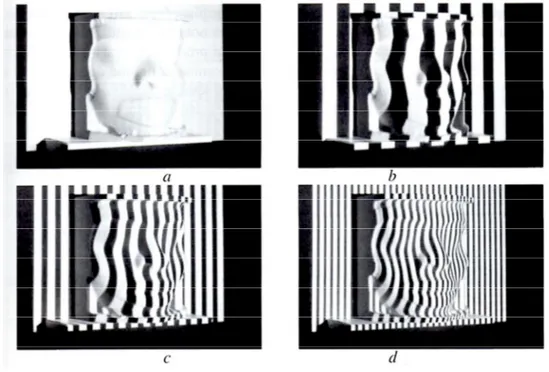
Figure 1.7 Example of a structured light scanning technique on an object surface: increasing fringe density is shown from image a) to image d) (Guidi et al, 2010) ... 16

Figure 1.8 Comparison between optical range imaging technique (Sansoni et al, 2009) .. 17

Figure 1.9 Two different range maps are first register by the identification of 3 pairs of homologous points ... 20

Figure 1.10 Filling holes on an acquired mesh ... 21

Figure 2.1 The same quantity is measured many times: σ is the precision error and it is random; β is the bias error and it is systematic ... 31

Figure 2.2 Error in measurement of a variable in infinite number of readings (Coleman, Steele, 1989) ... 32

(18)

Figure 2.4 The target used for resolution investigation: an example of low (in the middle)

and high (on the right) resolution instruments (Boehler et al, 2003) ... 34

Figure 2.5 The testing vase (Artenese et al, 2003) ... 35

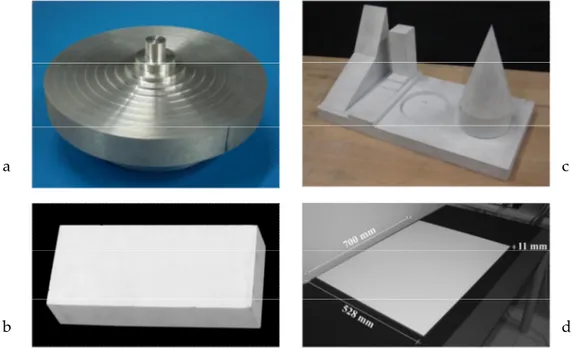
Figure 2.6 Test object used in the experiments to evaluate point resolution in Z (a) direction and in x,y one (b). some solids (c) and planes (d) are evaluated to testing accuracy and uncertainty ... 36

Figure 2.7 Origin of some typical uncertainties in 3D imaging systems (Beraldin, 2009) 37 Figure 2.8 Laser beam diffraction ... 38

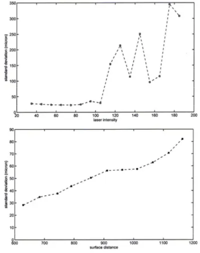
Figure 2.9 Noise standard deviation in relation to the variation of (on the top) scanner laser intensity and (on the bottom) of surface distance (Sun et al, 2009) ... 39

Figure 2.10 The reference surface used for the acquisition process ... 44

Figure 2.11 The Field Calibration System, parts nomenclature (Vivid manual) ... 47

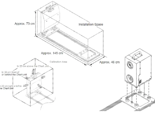
Figure 2.12 The Field Calibration System: the installation space, the calibration area and laser scanner connection (Vivid manual) ... 48

Figure 2.13 The calibration chart: on the top the calibration of the Wide lens and on the bottom Tele and Middle procedures are shown. ... 49

Figure 2.14 Glass sheet degree of freedom ... 51

Figure 2.15 Glass sheet fixing: clamps connections ... 53

Figure 2.16 Upper and lower shafts ... 53

Figure 2.17 Gears: XA 30 100 B3 Tramec S.r.l. ... 54

Figure 2.18 Bearings and their boxes insert into the frame: on the left the boxes are designed in blue, in green the bearings are sketched. On the right, their position into the up and bottom part of the frame ... 55

Figure 2.19 Shaft/frame connection... 56

(19)

Figure 2.21 The realized structure and its CAD definition ... 57 Figure 2.22 The scanning process with laser beam perpendicular with the reference surface, a first set up, before the support structure development ... 59 Figure 2.23 On the left: representation of the acquisition process; on the right: example of real scan. ... 60 Figure 2.24 An acquisition setting ... 62 Figure 2.25 An example of reduction process: on the left a visualization of the distances between two near points: it is possible to notice a wide dispersion in boundary parts.... 65 Figure 2.26 Principal components 3D space ... 67 Figure 2.27 Last square method: example of application in the bidirectional space... 67 Figure 2.28 Elaboration phase workflow ... 70 Figure 2.29 The acquisition process: two acquired frame as seen in PET. Scans are

acquired with a Tele lens at a distance of 600 mm (on the left) and 900 (on the right) ... 73 Figure 2.30 The acquisition process: two acquired frame as seen in PET. Scans are

acquired with a Middle lens at a distance of 600 mm (on the left) and 900 (on the right) 73 Figure 2.31 Area of the acquired frame in relation to scanning and focal distances... 74 Figure 2.32 3D graph of an acquired surface portion. Point’s Z coordinates are view as a color map; coordinate values are in mm... 76 Figure 2.33 dx and dy distanced between two near points are evaluated, in order to define local points resolution ... 76 Figure 2.34 3D graph on points distances in x (on the top) and y (on the bottom)

directions (all values are in mm) ... 77 Figure 2.35 Segment lengths in dependence on its position in the frame (column:

segment position which runs from 1 to 640): the first image corresponds to the first row, the second one to the meddle row (240) and the last one to the last row (480) ... 79

(20)

Figure 2.36 Segment lengths in dependence on its position in the frame (row: segment position which runs from 1 to 480): the first image corresponds to the first column, the second one to the meddle column (320) and the last one to the last column (640). ... 80 Figure 2.37 3D graph of the shifting between acquired points and the best fitting plane. All values are in mm ... 83 Figure 2.38 Standard deviation trend in function of the number of averaged arrays: Tele lens and scanning distance of 600mm ... 84 Figure 2.39 Acquired and reduced plane: from the difference between the reduced plane and the best fitting plane errors in coordinates’ determination are evaluated. Averaged and corrected plane: from the difference between the corrected plane and the best fitting plane errors in coordinates’ determination are evaluated ... 86 Figure 2.40 some acquisition frame: Tele lens, 600 mm of scanning distance and

changing tilt angles... 90 Figure 2.41 Only with some angular combination, the whole frame is completely

acquired; in all the other conditions only some central points are stored, and in many parts no points are present ... 92 Figure 2.42 3D representation of points coordinates in Matlab environment. Tele lens 600 mm of distance, α = 20°, β = 20° ... 93 Figure 2.43 Points resolution in X and Y directions, in function of their location in the frame. Tele lens, 600 mm of acquiring distance and (20°, 20°) of tilt angles ... 94 Figure 2.44 Segment lengths in dependence on its position in the frame (column:

segment position which runs from 1 to 640): the first image corresponds to the first row, the second one to the meddle row (240) and the last one to the last row (480). Tele lens, 600 mm of scanning distance and tilt angles of 20° each ... 95 Figure 2.45 Segment lengths in dependence on its position in the frame (row: segment position which runs from 1 to 480): the first image corresponds to the first column, the second one to the meddle column (320) and the last one to the last column (640). Tele lens, 600 mm of scanning distance and tilt angles of 20° each ... 96 Figure 2.46 Error representation in pseudo color, in function of points position in the acquired frame. Case study with geometric parameters α and β of 20° each. ... 98

(21)

Figure 2.47 Error standard deviation in relation to the number of arrays involved in the

mean process. Tele lens, 600 mm of acquiring distance and (20°, 20°) of inclination ... 98

Figure 2.48 Correction value (mm) in relation to point index. ΔS(0,0) values are indicated by a dot, while ΔS(20,20) values are represented by a cross ... 101

Figure 2.49 Difference (mm) between ΔS(0,0) and ΔS(20,20) arrays in relation to point index ... 101

Figure 2.50 Resolution values in relation to row position in the acquired frame. On the top is presented the first row, then the middle row and finally the last row. Scans are performed with a Tele lens, at 600 mm of distance and tilt angles of (40°,40°)... 104

Figure 2.51 Resolution values in relation to row position in the acquired frame. On the top is presented the first row, then the middle row and finally the last row. Scans are performed with a Tele lens, at 600 mm of distance and tilt angles of (60°,60°)... 105

Figure 2.52 Only the central portion of each frame can be used to perform the methodology, so that all acquired scans with similar operative conditions can have the same rectangular structure ... 107

Figure 2.53 Composition of two different scans: the first one performed at a less scanning focusing and the second one at an high distance. The black portion represents no acquired areas. The third image is the composition f the first two ... 109

Figure 3.1 Spherical System coordinates ... 115

Figure 3.2 Definition of plane and solid angle ... 116

Figure 3.3 Definition of radiance ... 116

Figure 3.4 The electromagnetic spectrum ... 117

Figure 3.5 Bourguer’s Law ... 121

Figure 3.6 Radiation emitted by a surface: spatial and directional distributions (Maldague, 2001) ... 121

Figure 3.7 Models of black bodies ... 122

(22)

Figure 3.9 Fraction of the blackbody emission in the wavelength band (0 to λ)

(Maldague, 2001) ... 126 Figure 3.10 The incident flux is divided into reflected flux, absorbed flux and

transmitted flux ... 127 Figure 3.11 Focal Plane Array Detectors configuration ... 138 Figure 3.12 Scanning System Configuration ... 140 Figure 3.13 Schematic depiction of an Infrared measure of related to an object (2)

through an infrared camera (4). 3 is the atmosphere and 1 in is the surrounding

environment ... 142 Figure 3.14 Thermal analisys of fiber orientation in composite materials and eliptical thermal obtained pattern (Maldague 1993) ... 147 Figure 3.15 A corroded bent pipe is inspected through a thermal-camera in order to detect the presence of defects: experimental set up (Maldague, 2001) ... 149 Figure 3.16 Experimental apparatus for thermographic inspection on turbine blades using internal stimulation: experimental set up (Maldague, 2001) ... 150 Figure 3.17 Sample geometries inspection through PPT and LT: stair veneered coating of variable thickness (Maldague, 2001) ... 151 Figure 3.18 Some examples of passive infrared thermography applied to buildings insulation defaults (Candoré, 2008) ... 152 Figure 3.19 Analysis of mineral based coating for buildings: experimental set up and thermal images acquired for different samples (Kolokotsa, 2012) ... 153 Figure 3.20 Some examples of thermography inspection on buildings surface: on the top the heat flux of the same building is presented (Hoyano, 1999) in summer (on the left) and in winter time (on the right). In the bottom part, a continuous surface monitoring is performed and the visible and infrared images are proposed (Sham, 2012) ... 154 Figure 3.21 Bridge deck delamination map created by thermal IR images (Endsley, 2012) ... 155

(23)

Figure 3.22 Infrared and visible images on power transmission equipments: a

transformer on the left and an electric cable on the right (Chou, 2009) ... 155 Figure 3.23 Thermal image of an inspected photovoltaic panel module: the central cell presents an unexpected behavior (Botsaris, 2010) ... 156 Figure 3.24 Thermal images of a subject talking on a hand-held mobile phone after 1 minute (on the left) and after 15 minutes (on the right) of talking (Lahiri, 2012) ... 158 Figure 3.25 Thermal image of left lower limb of a 28 years old male diabetic patient suffering from vascular disorder (a). (b) Temperature profile along the red line indicated shown in (a). An arrow indicate shows the lowest temperature (Lahiri, 2012) ... 159 Figure 3.26 Murals paintings of the abbey of “Saint Savin sur Gartempe” and the

thermographic inspection performed. The third image represents the IR image of the analyzed area: on the back wheel represented, some detachments are recognized

(Bodnar, 2012) ... 161 Figure 3.27 Mosaic inspection by thermography: a) building facade; b) IR image of the squared area in a); c) enlargement of the sqared area (Meola, 2005) ... 162 Figure 3.28 The main facade of the Cathedral of Matera and the location of the

thermographic data collection (Danese, 2010) ... 163 Figure 4.1 Djin Block No.9, in Petra (Jordan), a picture of the heritage monument (on the left), the acquired surface with a photographic texture (in the middle), and the surface with a thermographic texture (on the right) (Cabrelles, 2009) ... 171 Figure 4.2 Thermographic inspection and 3D reconstruction: a case study. On the left, an image fusion between IR a visible images is performed and an orto-thermogram is then obtained (in the middle). On the right, the final thermographic 3D representation is shown (Langüela, 2012) ... 172 Figure 4.3 The thermographic equipment including the specimen in the navigation cage. On the right, the thermogram used as a texture for the 3D acquired shape (Satzger, 2006) ... 173 Figure 4.4 Diagrams of thermography visualization: a conventional approach (on the left) and a video projection based approach (on the right) (Iwai and Sato, 2010) ... 174

(24)

Figure 4.5 Experimental result for a cluttered scene: on the left there are paint tubes under environmental light; in the middle the thermal image is shown; on the right the projection is applied (Iwai and Sato, 2010)... 174 Figure 4.6 Volume visualization at four different cutting levels. The MR information is clearly visible together with the surface temperature (Bichinho et al., 2009) ... 176 Figure 4.7 3D thermography example. Images from the top-left: the real object, the IR image, the surface acquired, the surface with the visible texture and the thermogram on the surface acquired (Barone et. al, 2006) ... 177 Figure 4.8 Methodology for data fusion: workflow ... 178 Figure 4.9 Example of Pts format files exporting ... 182 Figure 4.10 Points’ position in CCD Sensor and Array, in case of the whole frame

acquiring ... 185 Figure 4.11 Acquisition set up ... 186 Figure 4.12 The two thermographic devices used: the Flir ThermaCAM™ SC640 (on the left) and the Testo 882 (on the right) ... 188 Figure 4.13 Registration workflow ... 191 Figure 4.14 Temperature array displayed in Matlab environment ... 192 Figure 4.15 Laser Scanner Reference System. On the right in detail the CCD sensor: the acquiring object is considered as posed in front of it ... 194 Figure 4.16 Thermo Camera Reference System ... 195 Figure 4.17 Translations between the two reference systems: on the top the red point is laser scanner reference system origin; on the bottom thermal-camera dimensions. The total distance between the two reference systems origins is defined as sum of the two contributes ... 196 Figure 4.18 Constant movements (Translations) between the two reference systems .... 197 Figure 4.19 Camera and world coordinates systems ... 198

(25)

Figure 4.20 Rotation of world coordinates X’ and camera coordinate X, using the three Eulerian angles (φ, ϑ, ψ) with successive rotations about the X3’, X1’’ and X3’’’ axes ... 201

Figure 4.21 The central perspective projection (Yilmaz et al, 2008) ... 202 Figure 4.22 Complex shapes inspection: distance and angle effects (Ibarra-Castanedo et al., 2003) ... 205 Figure 4.23 Angle and distances influence in thermography inspections: on the left an experimental set up, on the right some temperature maps at angles of 20°, 50° and 80° (Tkáčová et al, 2010) ... 205 Figure 4.24 Blackbody distances and angle dependence in temperature reading (Tkáčová et al, 2010) ... 206 Figure 4.25 The problem of shape curvature in TNDT: an original and a rectified

thermogram example (Ju et al, 2004) ... 207 Figure 4.26 Heating analysis of a flat surface specimen (Maldague, 2001) ... 211 Figure 4.27 Heating analysis of a curved specimen (Maldague, 2001) ... 212 Figure 4.28 Beam geometry (Gaussorgues, 1994) ... 214 Figure 4.29 Correction workflow... 215 Figure 4.30 Geometrical quantities used for the definition of a correction factor ... 216 Figure 4.31 Graphical structure representing at the basis of the visualization

environment ... 220 Figure 4.32 Color maps used in the visualization environment ... 222 Figure 4.33 Experimental acquisitions: at the top, the visible and IR images acquired with the thermal-camera; at the bottom, the 3D acquired shape ... 223 Figure 4.34 Thermographic image in pixel coordinates, as viewed in Matab ... 224 Figure 4.35 3D thermogram as represented in Matlab environment: after the registration procedure, a temperature value is coupled with each acquired point ... 225 Figure 4.36 Thermographic 3D representation into a 3D software ... 226

(26)

Figure 4.37 The prototyped visualization tool: more color maps are created ... 227 Figure 4.38 The prototyped visualization tool: each triangle of the mesh of study

includes point’s temperature information... 228 Figure 0.1 Dimension Diagram (unit mm) ... 233 Figure 0.1 Standard deviation trend in function of the number of averaged arrays: Tele lens and scanning distance of 600mm (on the top) and 900 mm (on the bottom) ... 243 Figure 0.2 Standard deviation trend in function of the number of averaged arrays: Middle lens and scanning distance of 600mm (on the top) and 900 mm (on the bottom) ... 244 Figure 0.3 Standard deviation trend in function of the number of averaged arrays: Wide lens and scanning distance of 600mm (on the top) and 900 mm (on the bottom) ... 245

(27)

Introduction

Over recent years, Time Compression Technologies (TCT) are playing an ever increasing role and importance in the design processes and in project developments. Reverse Engineering (RE), Rapid Prototyping (RP), and Virtual Reality (VR) systems are currently widely used in industrial engineering fields as key tools to reduce product time to market and to improve product quality and performances, cutting down design costs and time. This is the reason why they play an important role in sustaining product innovation and industrial competitiveness.

Particularly, the old and well known design process has drastically changed thanks to the Reverse Engineering systems: in the previous processes, a new idea was developed and implemented within CAD (Computer Aided Design) environment and then converted into the final product; after the RE introduction, a 3D digital object description has been obtained starting from a real object. Design processes can be thus transformed, by changing design workflows, making processes easier, increasing efficiency and decreasing time product development.

These qualities imply that RE could be applied not only in industrial contexts, but also in many other different fields, making remarkable improvements. Biomedical,

(28)

cultural heritage, architecture and civil engineering are several of the most common RE application areas.

Laser scanners are some of the most used Reverse Engineering systems, since they can offer a dense point cloud describing almost any object shape complexity in a rather easy and fast acquisition process. Object acquisition process is based on the optical scanning of the object surface from different views, so that more range maps are acquired to describe the whole surface. A post processing phase, which is generally rather elaborate, arranges, organizes and then combines different scans. During this phase, some sub-phases are performed, to reduce data noise, to register acquired frames combining them together. At the end, a refining and filling holes phase follows to show a unique 3D model.

In this technical overview, this work shows two research focuses, which main purpose is to improve performances and application range of the scanning devices.

The first research topic is related to the analysis of error in point coordinates definition, calculated by a laser scanner system. All measuring systems show uncertainty level in provided data and, in particular for these tools, some errors can be observed by a surface noise on acquired surface. Even if in calibration procedures some instruments parameters can be set in order that the acquired surface has high accuracy levels, uncertainties of measurement are present anyway. Within this context, no unified

(29)

standards on error definition and well defined procedures for data correction are clearly identified. Supported by these considerations, the aim of the first part of this work is to identify data error related to images acquired by an optical laser scanner, and to propose a method for identifying the systematic portion of the error and for specifying errors correction arrays to compensate for systematic measurements errors.

The aim of this research activity involves the possibility to reduce errors in acquired data through a control and defined method. This feature seems to be promising and useful in many applications in which high accuracy level is strictly required, and when little details on object surface can be smooth in semiautomatic post processing procedures, together with errors. Cultural heritage and biomedical are some application fields in which the present methodology would lead to improve the acquisition process, along with the design and quality control phases of small components.

Moreover, the second research topic, related to scanning devices and their application procedures has been investigated. Currently, one of the most interesting research topics related to acquiring tools consists of integration process of data coming from different sources and including different information. In particular, within this context, a method for data fusion has been proposed in order to integrate 3D geometrical data, with temperature information, obtained by a thermographic investigation process.

(30)

Non Destructive Testing (NDT) are widely used in quality control processes in order to detect product defects and imperfections since early stages, in order to avoid and prevent any damages, that, sometimes, can lead to dangerous events or onerous and costly effects. Within this context, Infrared Thermography offers the possibility of detecting subsurface imperfections and changes in material composition, identified as a temperature difference, represented by a color map. Thanks to its efficiency in detect changes, non visible to the naked eye in an extremely fast way, this approach is currently widely used not only in industrial control quality processes, but also in architectural field and civil engineering inspections: in cultural heritage it is used as important support device for restoration processes, and in biomedical field as a fast diagnosis tool.

A method for data fusion has been developed, and shown in the present work, in order to integrate 3D geometrical data with surface temperature information. A temperature value is assigned to each acquired point, in order to provide geometry with more information and to read the infrared radiometric data according to the referenced geometry. In particular, in many cases, it can happened that the temperature information, that is generally provided by a color map image, are not easy to understand and to display their location in the visible image. This is the reason why a possible subsurface defect is not easy to detect. The integration between that kind of information

(31)

and a 3D shape information, acquired by a laser scanner tool, makes infrared thermography easier to understand.

A further considered aspect implies that radiation transmission is affected by dispersions due to the camera views and distances. The association of the 3D object geometry information is used to correct the thermographic datum and make thermography outcome independent from the acquisition setting up. On one hand, temperature values are associated with the referenced 3D point, so that defect detection is easier; on the other hand the 3D surface is used to make infrared inspections quantitative and not only qualitative.

The proposed data fusion process is expected to improve thermographic testing in many application cases , since a 3D thermography is analyzed in a multidimensional environment. Potential applications are identified both in civil engineering and in TNDT (Thermography Non Destructive Testing) processes. Moreover it should provide improvements in cultural heritage and biomedical inspections.

In the first part of this thesis, a brief introduction on Reverse Engineering systems and methods is presented. In Chapter 2, the developed methodology for error analysis and correction is described in detail.

(32)

The following parts concerns a first thermographic introduction on inspection techniques and methods and Chapter 4 indicates the data-fusion procedure and workflow.

(33)

1. Reverse Engineering: systems and processes

Reverse Engineering techniques are currently widely used, since they are able to define a 3D digitalized description, starting from a real physical object. The obtained 3D shape can be used in many different contexts and application: in particular, in new industrial product design process, these techniques, invert the traditional design process and workflows. In product design the CAD – CAM – RP loop often represents the starting point for a new product development or for a redesign and reinvent process. Moreover in many cases, such as car design, clay modeling is one of the most used techniques for new shapes definition and reverse engineering process is the only possibility to transform modeler idea into a 3D digitalized representation. Quality control process is another industrial field in which such technology is currently widely used, in order to compare the final product geometrical features with designed ones (Sansoni et al 2009).

Reverse engineering systems are also commonly used to design customized product, with a user-oriented design method: sport helmets are an example. In biomedical field RE tools helps to design patient prosthesis or anatomical parts (Gibson 2005; Fantini et al. 2012; Fantini et al. 2013).

(34)

Finally, in cultural heritage, Reverse engineering is a fast and efficient tool to analyze artworks, and it is widely used in restoration processes or to make copies, or to develop data information or to design the transportation process of an artwork (De Crescenzo et al 2008a; De Crescenzo et al 2008b; Persiani et al 2007; Curuni Santopuoli 2007).

During an acquisition process, 3D point’s coordinates are organized in point clouds that take into account point connections and neighborhood information (Beraldin, 2009). All these acquired data can be represented in many different ways and the simplest one consists in a uniform (u,v) parameterization of a depth map. It is arranged as a matrix whose row and column indexes are function of the two orthogonal scan parameters (X, Y). The matrix cells can contain some more information on continuity between points, point’s depth measurement (Z), calibration quantities and any other attribute, such as color data.

Figure 1.1 Some representation of a 3D point cloud: a) gray scale image range map; b) 3D point connected as a wire-mesh; c) a mesh artificially shaded; d) representation

(35)

The simplest 3D representation depth information can be represented in a grayscale image; moreover a triangulation mesh can be used to display a range image, or using topology dependent slope angles to represent the local surface normal on a given triangle. Surface normal directions are generally used to artificially shade the acquired mesh, in order to highlight and reveal surface details (Figure 1.1).

Figure 1.2 Reverse Engineering process and output Real Object Point Cloud VRML STL Rapid Prototyping NURBS CAD Mesh Virtual Reality

(36)

Object geometrical description is achieved by many different steps, starting from the acquisition of range maps that described the specimen surface as a discrete point cloud. Data acquired are elaborated and post processed in order to create a 3D surface composed by triangular elements (called mesh) that approach the real surface shape. Such polygonal triangular mesh can be stored in a stl (Solid To Layer) file format, which allows exchanges with CAM (Computed Aided Manufacturing) and RP (Rapid Prototyping) tools. Moreover 3D models can be used in Virtual Reality applications using VRML (Virtual Reality Modelling Language) as exchanging file format. A further development can be the realization of a NURBS surface that allows CAD modeling. The whole acquiring and elaboration process is presented in Figure 1.2.

(37)

1.1 Reverse Engineering tools

Many methodologies and systems for a semi automatic 3D data acquisition are currently used (Figure 1.3): according to the specific case study a technique will be more promising than another one. The choice on what scanning technique to use is dependent on object surface features: its dimensions, its surface complexity, the presence of holes or undersurfaces, reflective or transparency properties, its transportability and accessibility and the potential necessity to acquire other information, such as surface color, required accuracy and performances, time and costs.

(38)

In general Reverse Engineering techniques can be classified into two main groups in relation to the request or not of a contact between the acquisition device and the object. In contact techniques, point coordinates are evaluated thanks to a contact between the specimen and a probe; used sensors are generally investigating probes that go through object’s surface into the 3D environment with a high precision level and with known trajectories. Coordinate Measuring Machines (CMM), articulated arms, and piezo sensors are some examples: they are characterized by high data precision and repeatability, even if they take a long time to scan a complex shape. Moreover, since a contact between object and probe is required and in many case studies it is not possible, they cannot be used in cultural heritage applications or for soft component scanning.

Another group of scanning systems measure points coordinates without a direct instrument – object contact, but an energy flux is radiated on specimen itself and the transmitted or reflected energy is the measured.

Computer Tomography is one of the most used transmission method: X-rays pass through analyzed object and their transmitted portion is measured. Different cross section planes are stored as DICOM images: data accuracy level depends on the slicing process. The different gray color level indicates object internal composition. A final object volumetric representation is obtained (Figure 1.4). This technique is not effected by specimen superficial and reflective properties, moreover it is able to detect object

(39)

internal holes and structures; on the other hand instruments used are particularly expensive and X-ray emission is required.

Reflective scanning devices can be optical or non optical, like sonar or microwave radar that measure object distance evaluating the time that an emitted wave (or impulse) takes to come back after its reflection on object surface.

Optical reflective systems are distinguished between active and passive tools: while the first ones are the most used acquiring devices, since they are able to detect in a fast and precise way a large data quantity, passive scanning systems used instead light naturally present in a scene. Photogrammetry, as example, is based on the acquisition of many photo images, with a calibrated camera, and taken from different points of view that are processed in order to define points coordinates. The elaboration pipeline consists basically in camera calibration and orientation, image point measurement, 3D point cloud generation, surface generation and texture mapping (Sansoni et al, 2009).

(40)

Optical active scanning systems send an energy flow on object surface and its geometry is measured on the basis of the definition of an optical quantity of reflective energy portion (Scopigno, 2005; Scopigno, 2003). A laser or a board spectrum source is used to artificially illuminate a surface, in order to acquire a dense point cloud using triangulation, time-of-flight or interferometric methods.

In time-of-flight laser scanner, points coordinates are measured on the basis of the time that emitter laser beam put to come back to the sensor after its reflection on object surface (Figure 1.5) according to Eq 1.1.

= ∆ ; c ≈ 3*108_m/s _{Eq 1.1}

Acquired data accuracy is related to time measurement precision and distances that these instruments are able to detect goes from some meters to some hundreds of meters, with a decreasing accuracy level.

(41)

On the other hand, in optical triangulation laser scanner systems, object points are defined by a trigonometrical process, between the relative positions of the CCD sensor and laser source and measuring from time to time the reflection angle (Figure 1.6), as indicated in Eq 1.2. Both single-point triangulators and laser stripes belong to this category.

=

tan( + ) Eq 1.2

Laser triangulators accuracy and their relative insensitivity to illumination conditions are some of the main advantages related to this scanning principle. Single-point laser scanner are widely used in industrial applications for distances, diameters or thickness measurements. On the other hand laser stripes are mostly used for quality control and reverse modeling of heritage.

(42)

The triangulation approach is also used by structured light based 3D sensors. They project a bi-dimensional patterns of non-coherent light, which move in horizontal direction and scan the whole object surface (Figure 1.7). The surface shape distorts projected fringes that are acquired by a digital camera and elaborated in a range map (Guidi et al., 2010).

Interferometric methods project a spatially or temporally varying pattern into a surface, followed by mixing the reflected light with a reference pattern. Since their resolution is a fraction of laser wavelength, acquired surface quality is very accurate and they are widely used in surface control, microprofilometry or in CMM calibration procedure.

Figure 1.7 Example of a structured light scanning technique on an object surface: increasing fringe density is shown from image a) to image d) (Guidi et al, 2010)

(43)

A final scheme of optical scanning devices is shown in Figure 1.8: their strength and weakness are always take into exam when a method should be chosen in a defined application.

(44)

In this technical panorama, many research activities are focused on the integration of data coming from different sources, in order to provide more information in the same 3D model. Some examples regard the integration between volumetric and superficial data (Fantini et al., 2005), or data coming from instruments with different resolution level (De Crescenzio et al, 2010). Other works are related on instrument performances and error detection (Some detailed example will be presented in Section 2.2)

1.2 The acquisition pipeline

The process from a real object to a 3D shapes is composed by different steps that can change in relation to the instrument and technology used in the reverse engineering process. Considering acquiring object surface with an optical laser scanner, the output of each scan is a range map, that is to say a 3D array of acquired points, which can be post processed as a point cloud or as a triangulated surface (mesh).

The acquisition pipeline is composed by some consecutive following steps that are listed below.

1.2.1 Scans planning and acquisition process

Each scan output is a range map describing the object surface portion in the acquisition frame. A complete 3D description of the whole specimen is obtained from

(45)

many different range maps acquired from different points of view. In this context the first phase consists in a detained planning of how many scans are necessary to acquire the surface of interest and where such scans should be taken. This procedure should tend to reduce the number to necessary scans in order to reduce time and costs, and, at the same time, the final model would be without holes or not acquired parts.

Since acquired range maps will be then register together in order to obtain an unique model, it is important to have about 30% of overlapping points between two subsequent point clouds. Moreover, in order to increase final mesh quality, it is important to perform the scanning process with the laser beam as perpendicular as possible to the object surface.

1.2.2 The registration process

The acquisition phase output consists in many different range maps, describing the correspondence portion of the object surface, and each of them has its own reference system. The following phase aims to register all acquired point clouds, saving them in a unique and common coordinate reference system.

A first registration process is performed during the acquisition phase and consists in the identification of at list 3 homologous point belonging to two different scans (Figure 1.9): the software is then able to perform a point registration minimizing the gap between the two considered point clouds.

(46)

Once this first phase has been performed, all acquired scans are involved in a refinement registration process, whose aim is to improve the alignment between all range maps at the same time.

1.2.3 Range map merge and refining phases

After the registration process, all acquired frames are each other registered, but they are stored as different shells. A merge phase is then performed in order to obtain a unique mesh, in which the acquired range maps are mixed together. Redundant surface Figure 1.9 Two different range maps are first register by the identification of 3 pairs

(47)

portions are removed and for each of them the elaboration software considers only the range map portion that best fit that surface patch.

Before this phase some cleaning procedures are performed, in order to remove from each shell some triangles describing no object parts, but the surrounding environment. Moreover boundary points, containing more surface distortions or errors are similarly removed. Non manifold triangles, small clusters, redundant surfaces, long spikes are some of the most common error typologies.

Some holes are then closed and a smooth procedure is performed, in order to remove noise (Figure 1.10).

During the acquisition process many points are obtained to describe a surface portion. In many case studying they are too much and even if a point reduction is performed no surface details are lost and, on the other hand, file size can be much

(48)

thinner. Point are remove on the basis of surface curvature, so that at the end of this process, their density is not uniform and more points are used to describe more complex and non uniform surface portions.

The final 3D model is an exact copy of the real object as concerns its geometry, shape and dimensions. In many applications a photo is also acquired and then registered on the final mesh as a texture, so that is color appearance is represented as well.

(49)

2. Experimental Error Compensation Procedure

Laser Scanner instruments are widely used in a widespread range of applications and cases, thanks to the possibility of acquiring a large number of points in very few seconds and are capable to describe surfaces of almost every kind of complexity and shape. This feature allows underlining a lot of case studies which use gives the possibility to reduce time in product design and improve quality processes and testing. In spite of these considerations, the employment of scanning instrument is connected to some preliminary considerations leading to a more aware use of those tools.

First of all, some hundreds of thousands of points on object’s surface are acquired at the same time. However, it may occur that some useful points are not directly acquired (such as corners or borders), and it is possible to reconstruct them in post processing phase, identifying the other points in range map. A real surface, which is a continuous surface, is numerically changed into a discrete surface and not all surface points are thus acquired (only some of them) and the others are deducted by a software procedure. This has effects on the definition of surface edges. Conversely, it may happen that the same part is acquired many times in different scans, from a different view: so it is described by different point’s clouds and in each of them it is impossible to have

(50)

exactly the same point’s coordinates. During post processing procedure, and in particular during the merge one, only one patch of one range map is selected to describe such surface portion.

Another interesting source of uncertainties in the acquiring procedure arise from the fact that laser scanners, like all measuring instruments, introduce some errors in determining points coordinates, so that if we acquire twice the same surface, under the same conditions, data obtained will never be exactly the same. This is caused by many factors, internal or external to the instrument itself, from the reflective properties of object’s surface and operative conditions, to laser scanner calibration and manufacturing features.

All these uncertainty reasons can be grouped into two different classes: a random component and a systematic component. Whereas the random part of error, in each scan, changes in module and sign, so that it is not possible to pre-determine it, the systematic component of error, in principle, can be identified, due to its property to maintain a homogeneous trend. In operational cases, these errors are clearly visible in the acquired mesh as a superficial noise.

Tools for noise reduction and smoothing procedure are present, in common commercial elaboration software, and they apply mathematical transformations which do not take into account errors nature and causes. For these reasons, it may happen that

(51)

some little details, present on object surface, are smoothed like a noise disturb, so that they are missing in the 3D representation.

By these considerations, and to overcome the issue above mentioned, an experimental and repeatable methodology is proposed to identify and correct the systematic part of the error in data acquired by an optical triangulation laser scanner, in a well-controlled manner.

Exploiting a reference surface, under well-defined operative conditions, systematic errors are determined in order to reduce their impact on further scans under similar conditions, improving scanning performances in terms of accuracy. A repeatable correction procedure is thus defined, in order to reduce shell noise, caused by the systematic portion of error and without any lost in detail due to an uncontrolled smoothing process. Finally, a parametric library of arrays for error reduction is created according to scanning operative conditions and surface orientation (Eq 2.1): a different array (ΔS) is defined according to acquisition distance d, laser scanner lens f used in the particular application and surface normal orientation (defined by angles α and β). Each point (i,j) of the acquired frame is corrected with its homologous value in the reference array.

∆S = ( i, j, d, f, α, β) Eq 2.1

In spite of an ever increasing use of RE technologies, unified standards and certifications for the evaluation of laser scanner’s performances and for determining

(52)

measurement’s repeatability, accuracy or precision are not yet defined. Moreover, no standards and unified procedures are certified in order to reduce instruments measuring errors.

Nevertheless, instrument’s periodical calibration plays a fundamental role in verifying and setting many internal scanning parameters and reducing part of the acquiring error.

In this chapter, a method for error correction is presented: first of all, scanning errors and performances are mathematically analyzed and then methodologies for error evaluation and accuracy increasing available in literature are taken into account. A correction procedure is then proposed and analyzed.

2.1 Mathematical analysis of errors

The evaluation of instrument performances and measurements accuracy are associated to theoretical definition of some basic concepts related to error characterization and uncertainties.

The absolute error of a measurement is the difference between a measured value

y* and the real one y (Eq 2.2):

∆ = ∗₋ _{Eq 2.2}

Measurement relative error is the ratio of the absolute error to the actual value (Eq 2.3):

(53)

= ∆ = ∗₋

Eq 2.3 In practical cases measurement real value is unknown and the measured value is the true conventional used one. For this reason it is important to evaluate a range which the actual value is located in: this lead to the definition of the limiting error, which is the smallest range around the measured value y*, containing the real value y (Eq 2.4):

∗_{− ∆} _{≥ ≥} ∗_{+ ∆} _{Eq 2.4}

Considering measurement errors in repeatable experiments, two different types of error are analyzed: a division into random and systematic error is made. The Systematic error (also known as bias), is the difference between the mean value calculated from an infinite number of measurements of the same quantity, carried out under the same conditions, and its actual value. Investigating results of the same repeated measurement, this error quantity changes its sign or value according to a specific law or function.

The error component is commonly called random error and it is defined as the difference between the result of an individual measurement and the mean value calculated from an infinite number of measurements of a quantity, carried out under the same conditions.

Errors types above defined refer to the results of individual measurements. Indirect measurements are those measurements in which the model is provided in form of function of input quantities. In such cases, the error is defined according to the law of

(54)

error propagation: an output quantity error, inherent to known errors of input quantities, can be measured by the methods of increments or the methods of the total differential. The method of increment, the exact method, consist of determining the increment of a measurement model function for the known increment of input quantities. For complicate measurement models, error evaluation becomes a long process and therefore it’s evaluated by approximated methods, such as the total differential method. It is based on the expansion of the studying function as a Taylor series around the point defined by the actual (conventionally true) values in input (Minkina, 2009).

Uncertainties in measuring processes generates doubts in results itself and they express the lack of accurate knowledge of the measured quantity. In detail, the standard uncertainty of a measurement is the uncertainty of measurement values, that specifies the dispersion of the values that could reasonably be attributed to the measured quantity that can be expresses in the form of the standard deviation (ISO ENV 13005).

To estimate measurement quantitative accuracy, some model inputs are considered as random variables that are described by a probability distribution function. For estimating measurement accuracy, the most important statistics of random variables are the expected value and the standard deviation value. The expected value E(X) of a discrete random variable X, which values xi appear with probabilities pi is (Eq 2.5):

(55)

( ) = _{Eq 2.5}

The set of measured values xi is a finite N-element set. The expected value is substituted by its estimator, that is the arithmetic mean from N independent observations (Eq 2.6):

̅ = 1 Eq 2.6

A random variable standard deviation is the positive square root of the variance (Eq 2.7):

( ) = [ − ( )] Eq 2.7

In practical problems an estimator of standard deviation, called experimental standard deviation (Eq 2.8) is used (Minkina, 2009, ISO ENV 13005):

( ) = 1

− 1 ( − ̅) Eq 2.8

2.1.1 Resolution, accuracy and precision

Some more basis quantities are now introduced: resolution, precision and accuracy.

Resolution is the smallest spatial step that the instrument is able to detect; it can be measured in X, Y and Z directions.

(56)

In determining point’s coordinates through a series of measures, precision (or uncertainty) is standard deviation of that measures: a high precision corresponds to a low standard deviation, and it represents random component of error. Instead, accuracy is instrument capability to give, at each measure, a data near to the real value (Azzoni, 2006; Taylor, 2004; Webster, 1999).

The degree of inaccuracy (or the total measurement error δ) is the difference between the measured value and the true value. The total error is the sum of the bias error (β), which is systematic, and the precision error (σ) that is the its random component (Coleman, Steele, 1989). A number of measurements, one after the other, of the same variable, whose real value is V, that is absolutely steady, is performed (Figure 2.1). Since the bias (β) is a fixed error, it is the same for each measurement. The precision error is a random error (σ) and will have a different value for each measurement. Since the total error is the sum of the two components, it will be different for each point (Eq 2.9):

(57)

Considering to acquire N measurements and N approaches to infinity, data would appear as Figure 2.2. The bias would be given by the difference between the mean value of the N readings (μ) and the true value of X, whereas the precision errors would cause the frequency of occurrence of the readings to be distributed about the mean value.

Figure 2.1 The same quantity is measured many times: σ is the precision error and it is random; β is the bias error and it is systematic

(58)

2.2 Error analysis in scanning processes

In spite of an increasing use of scanning devices, and in particular of laser scanner systems, a unified standard or a certified method for performances evaluation does not exist yet. Nevertheless, the necessity of increasing instrument accuracy and measurement repeatability is one of the most pursued research topic. Within this context, instrument calibration plays a fundamental role in defining some instrument internal parameters. Accuracy, repeatability measuring uncertainties can be defined, after a calibration procedure: conceptually, if the geometrical description of the object is defined, the deviation of each point on object’s surface can be considered as an accuracy indicator. From this concept, it is possible to find a lot of experimental techniques, with

Figure 2.2 Error in measurement of a variable in infinite number of readings (Coleman, Steele, 1989)

(59)

the aim to define the level of reliability of acquired data, and with the aim to verify and compare different instrument’s performances.

Within this context, many experimental techniques are available in literature, in order to define measure confidence level, according to data true value, and to compare performances of different scanning instrument. Boehler et al (2003) perform some tests on different scanning devices (triangulation and time of flight): plane surfaces of different reflectivity are scans from different distances and a best fitting plane is created in order to get indications of the range measurements noise. Moreover, several tests are set up scanning white sphere as targets, with the aim to get information on scanning accuracy. Results show that even if a laser scanner shows better results, this does not means that the instrument is better at all. Instrument reliability has dependences with the specific application and case study. Test performed concerns angular accuracy, which is evaluated scanning two equal spheres, posed at the same distance from the scanning device, but in different positions (Figure 2.3): their horizontal and vertical length is measured and compared.

(60)

As regards resolution analysis, some information is obtained by scanning a target with small slot on its front panel (Figure 2.4): high resolution scanning devices are able to detect the bottom panel too, when the laser beam get through the front panel.

Some more information are available comparing instrument performances when edge effects and surface reflections occur. Within this context, the presence of corners lead to the identification of wrong points, due to laser beam deviation, in proximity of

Figure 2.4 The target used for resolution investigation: an example of low (in the middle) and high (on the right) resolution instruments (Boehler et al, 2003)

(61)

discontinuities: the acquisition of a sharp edge gives the possibility to test all the points that are located in a wrong position. Finally, surface reflective properties are due to some errors and uncertainties estimable by comparing plane of different material and color.

Artenese et al 2003, has the aim to define instrument precision value in order to compare three different techniques: optical triangulation laser scanner system, digital photogrammetry and mechanical feeler. A vase has been tested, whose vertexes are determined analytically in a very precise way (Figure 2.5). After the acquisition process the three point clouds have been compared: results shows that points in the middle parts are affected by a less gap than boundary points. Moreover, acquired range maps have different density: photogrammetry and mechanical feeler meshes have lower resolution levels.