Balance-Sheet Based and Unconventional Policies in an Agent-Based Model

Working Paper

Balance-Sheet Based

and Unconventional Policies

in an Agent-Based Model

This project has received funding from the European INNOVATION-FUELLED, SUSTAINABLE, INCLUSIVE GROWTH

27/2018 June

Giovanni Dosi

Scuola Superiore Sant’Anna

Mattia Guerini

OFCE-SciencesPo and Scuola Superiore Sant’Anna

Francesco Lamperti

Scuola Superiore Sant’Anna and Fondazione Eni Enrico Mattei

Mauro Napoletano

OFCE-SciencesPo, Scuola Superiore Sant’Anna and SKEMA

Andrea Roventini

Scuola Superiore Sant’Anna and OFCE-SciencesPo

Tania Treibich

Deliverable DD 6.5

WP 6

Report: Schumpeterian & Keynesian policies

Balance-Sheet Based and Unconventional Policies in an

Agent-Based Model

Giovanni Dosi

, Mattia Guerini

, Francesco Lamperti

,

Mauro Napoletano

, Andrea Roventini

, Tania Treibich

June 4, 2018

Abstract

In this paper we shed more light about the interactions between accounting policies and uncon-ventional monetary policies. By employing a modified version of the Schumpeter meeting Keynes Agent-Based model (KS model) we study the effects that Mark-to-Market (MtM) accounting stan-dards might have in terms of financial stability, economic growth and sustainability of public finances. We also study the effects of Quantitative Easing (QE), modeled as the intervention of the central bank for the clearing of bad-debts accumulated by the financial institutions. Our re-sults suggest that the Mark-to-Market standard might generate instability in the credit side of the economy because of its pro-cyclical nature; the QE instead, being counter-cyclical might coun-teract the negative effects. However, a QE policy alone, does not outperform a baseline scenario with historical accounting standards and without unconventional monetary policies, suggesting that QE might be useful to counteract peculiar crisis events but shall not become a conventional instrument to be employed at any occasion.

∗_{Scuola Superiore Sant’Anna g.dosi@santannapisa.it}

†_{OFCE-SciencesPo and Scuola Superiore Sant’Anna mattia.guerini@sciencespo.fr}

‡_{Scuola Superiore Sant’Anna and Fondazione Eni Enrico Mattei f.lamperti@santannapisa.it} §_{OFCE-SciencesPo, Scuola Superiore Sant’Anna and SKEMA mauro.napoletano@sciencespo.fr}

¶_{Scuola Superiore Sant’Anna and OFCE-SciencesPo a.roventini@santannapisa.it}

1

Introduction

Accounting standards are important policy choices that might have real macroeconomic implications.

As a matter of fact, in the past, large financial and economic crises brought to a reconsideration of

these policy choices. At the two poles of such a choice stand two opposite alternatives: the historical

value accounting principle vis-à-vis the mark-to-market accounting principle (also known as fair

value principle).

While before the Great Depression and until 1934, firms and banks had great flexibility about

re-porting the asset valuations they held in their portfolios, by the early 1940s the historical value

ac-counting had become the standard.

Also as a result of regulation, in the 1970s however, the

introduc-tion of derivative contracts and other financial instruments induced the SEC to reconsider the usage

of historical value accounting and to allow banks adopting the mark-to-market principle for the

eval-uation of futures and other foreign exchange contracts. During the 1980s, the fair value accounting

principle was extended also to debt and equity contracts for the banking sector and by the 1990s, the

mark-to-market accounting became the standard since the FASB required “all entities to disclose the

fair value of financial instruments, both assets and liabilities recognized and not recognized in the

statement of financial position, for which it is practicable to estimate fair value” (see

FASB

,

1991

).

In the recent years however, economists have been raising concerns about the fact that

mark-to-market accounting principles might have played an important role in the fast amplification of the

financial crisis. The fall in the values of a large fraction of securities which were strongly correlated

with house prices, led to large and almost immediate devaluations of the asset side of the banking

sector, due to the adoption of the fair value accounting standard, and have strongly influenced the

ability of the banking industry to continue to perform its basic lending activity. This of course have

had important real effects as also documented by

Heaton et al.

(

2010

);

Bhat et al.

(

2011

);

Kolasinski

(

2011

) and might have played a role in lowering the liquidity of the market. All in all therefore,

questions concerning the macroeconomic effects of the mark-to-market accounting principle, are

im-portant matters that naturally correlates with other questions about market liquidity,

Brunnermeier

and Pedersen

(

2009

), credit cycles (see

Kiyotaki and Moore

,

1997

), macroprudential regulation

Galati

and Moessner

(

2013

) and unconventional monetary policy

Rodnyansky and Darmouni

(

2017

).

In the last decade indeed the introduction of unconventional monetary policies by several Central

Banks have been of fundamental role to keep the value of long-term yields to low levels (

Krishna-murthy and Vissing-Jorgensen

,

2011

;

Duca

,

2013

), to counteract the low credit supply (

Rodnyansky

and Darmouni

,

2017

), and to dampen the downward phase of the credit cycle (

Bhattarai and Neely

,

2016

).

_{The common wisdom of monetary policy showed its greatest limitation when the short-term}

interest rates hit the zero lower bound (ZLB). To react to the liquidity trap, central banks from all over

the world have been forced to design new policy instruments and to experiment new transmission

mechanisms for monetary policy to be effective: the Quantitative Easing policy is the most evident

form of this.

1_{After the Securities and Exchange Commission (SEC) forbade revaluation of assets in the balance sheets in 1934. For a}

complete historical narrative of the accounting principles used in the US seeSEC(2008).

2_{See alsoGuerini et al.(2018) for a discussion about how the QE might have had different effects in US and EU also due}

Nowadays there are therefore two ways of implementing monetary policies (see

Borio and Zabai

,

2016

). The first comprehends interest rates policies, the second points to balance sheet policies. The first

set includes the conventional Taylor rule (whose effects have been extensively discussed by means

of empirical models

Angrist et al.

(

2013

), neoclassical models

Galí

(

2015

) and evolutionary models

Dosi et al.

(

2015

)), the new forward guidance principles (which have mostly drawn the attention of

empirical and experimental economic research (see respectively

Swanson

,

2017

;

Ahrens et al.

,

2017

))

and the maturity transformation programmes (see

Ehlers

,

2012

); these policies aim at controlling and

fixing some reference short-term interest rate, to which the yield curve is linked, and to affect in

turn macroeconomic fundamentals. The second policy set includes instead the large asset purchase

agreements, the non-standard supplies of funds as well as the newly introduced reserves policies –

which are also macro-regulatory policies. These last tools have been only recently introduced and

their effects are far from been fully investigated and understood.

In this paper we try to shed more light about the interactions between accounting policies and

unconventional monetary policies. By implementing policy experiments in a new version of the

Schumpeter meeting Keynes Agent-Based model (K+S model, see

Dosi et al.

,

2010

,

2013

,

2015

;

Lam-perti et al.

,

2017

) we indeed analyze the transmission mechanisms of different policies – such as

mark-to-market accounting for banks assets and quantitative easing policies – and the aggregate

macroeconomic effects that they generate. This paper is organized as follows: section

2

reviews the

events of the last decade and the policies implemented by the four work major central banks (FED,

ECB, BoE, BoJ); section

4

presents some specific equations of the model and discusses the new parts

of the model that have been introduced with the aim of evaluating the above mentioned policies; in

section

5

we perform the policy evaluation exercise and presents the result. Section

6

concludes. A

final appendix

A

is dedicated to the presentation of the full model, which emerges from the merge of

two versions of the K+S agent-based model (see

Dosi et al.

,

2015

;

Lamperti et al.

,

2017

).

2

Conventional and Unconventional Monetary Policies at the Four Major

Central Banks

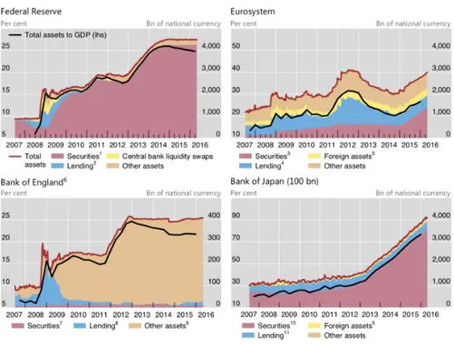
Let us start by discussing how unconventional monetary policies were implemented at 4 different

central banks in the last decade. In figures

1

and

2

it is possible to see that notwithstanding the

attempt of collecting the available central bank policies under common features and objectives, the

balance sheets compositions (as well as their size) are still quite heterogeneous for each economic

area. This is due to the fact that the different central banks carried out different policy combinations

and had to overcome different situations.

3_{Among the balance sheet policies,Borio and Zabai(2016) recognize also the possibility of an intervention of the Central}

Bank onto foreign exchange markets to affect the exchange rate, but this tool is not discussed here.

4_{For example, in EU and UK the central bank aims at a pure inflation targeting while in US and in Japan also a output}

is, more or less explicitly, targeted. Also, when the crisis hit, the respective levels of public debts to GDP in US and UK were not as high as in many EU economies or as in Japan.

Figure 1:

2.1

FED Policy Tools

Since the advent of the crisis, the way of doing policy at the Federal Reserve has undergone

ma-jor transformations.

Nowadays, we can classify the tools employed by the Federal Reserve under

four main categories: the first two are interest rate policies while the third and fourth instruments are

balance-sheet policies. Some of these measures have been switched off as the 2008 crisis was fading

away, but they might be restored in case of a new crisis event.

Open Market Operations (OMO) This is the standard (pre-crisis) method of doing monetary policy

via acquisitions and sales of securities to control interest rates and in turn to affect investment and

consumption. These operations can be either permanent or transitory: the first accommodate the

longer-term factors driving the expansion of the Federal Reserve’s balance sheet – mainly currency

before the crisis and reserves during the crisis; the second aim at addressing reserve needs that are

deemed to be transitory in nature and that can easily be fixed by means of REPOs and Reverse REPOs

contracts.

Maturity Extension Programme (MEP) These are measures that, by prolonging the maturity of the

portfolio of assets held by the central bank, dampens the upward pressure on the long-run interest

rates. In particular, the FED during the crisis – by means of two interventions in 2011 and 2012 – sold

a total of 667 Billions USD short-term Treasury securities with maturity lower than 3 years and in

exchange, used the same amount of money to buy Treasury securities with maturity between 6 and

30 years.

Crisis Response Operations (CRO) When the liquidity trap was reached and the target nominal

rate hit the ZLB during the crisis, standard OMO were ineffective for the control of investment and

consumption. New methods for the liquidity provisions have therefore been designed by the FED.

Among them we can distinguish between liquidity provision to banks and other financial

institu-tions and liquidity provision to borrowers and investors in key credit markets. In the first set of

tools there are the Term Auction Facility (TAF), the Term Securities Lending Facility (TSLF) and the

Primary Dealer Credit Facility (PDCF), all of which are aimed at increasing short term liquidity in

exchange of high-quality collaterals. In the second set there are the Commercial Papers Funding

Fa-cility (CPFF), the Money Market Investor Funding FaFa-cility (MMIFF) and other instrument aimed at

providing funds to professional investors and special purpose vehicles in exchange of eligible

collat-erals.

Asset Purchase Agreements (APA)

_{. These operations expand the standard OMOs and consist in}

straight acquisition of assets by means of the central bank. From 2008 onward, the FED had

in-tervened with four large scale asset purchase agreements, beginning to acquire 175 Billion USD of

obligations and other 1.25 Trillion USD of guaranteed Mortgage Backed Securities from Freddie Mae

and Freddie Mac in the 2008-2010 period. In 2009 it also extended the QE to long-term Treasury

se-curities, buying 300 Billion USD and it increased the acquisition to 600 Billion USD in the 2010-2011

period. Furthermore, starting from the end of 2012 (with the near end of the Maturity Exchange

5_{This section draws from scattered information available athttps://www.federalreserve.gov.}

6_{This practice has also been more commonly dubbed Quantitative Easing (QE). Here we will use the two terms as}

Programme) the FED started to buy MBS and Treasury securities at a monthly rate of 85 Billion USD

each month, until the end of 2014 when all the purchases of new securities have been stopped.

2.2

ECB Policy Tools

Also in the European Union the available monetary policy measures have been largely expanded

as a reaction to the prolonged crisis: long-term refining operations as well as asset purchases

pro-grammes have indeed been carried out also in the EU. However in the first attempts to respond to

the crisis (2009-2012 period) only few resources have been dedicated to unconventional monetary

programmes; after 2014 the amount of resources has instead been increased substantially.

The first

two measures below can be thought as interest rates policies while the last one falls into the balance

sheet policies category.

Open Market Operations (OMO) This is the bulk of the EuroArea monetary policy instruments

and consists in buying and selling securities in exchange of weekly (Main Refinancing Operations)

or three-months (Longer Term Refinancing Operations) liquidity. Also, institutions can deposit or

obtain overnight liquidity at a respectively lower and higher interest rates (Deposit Facility and

Marginal Lending Facility). Also, the ECB requires to banks and financial institutions to hold

de-posits on accounts with their national central bank which compose the minimum required reserves

(MRR). All in all, these measures form the interest rate corridor system and allows the ECB to set the

short-term interest rates in order to reach the 2% inflation target.

Long Term Refinancing Operations (LTRO) In June 2014 and January 2015, the ECB has introduced

two new policy instruments that shall allow to manipulate also long-term interest rates. These two

instruments are the Targeted LTRO and the 3-years LTRO. The first has been a measure by which

the ECB have guaranteed financing up to 4-years to the banks at particularly favourable conditions

and where the amount that banks could have borrowed, was linked to their outstanding loans to

non-financial corporations and households. The second was instead an instrument by which the

ECB provided a 3-year lending to the financial institutions accepting in exchange also lower-quality

collaterals and by by allowing reduced reserves ratios. These measured have allowed the ECB to

keep relatively low interest rates during the period from mid-2014 to mid-2016.

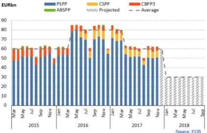
Asset Purchase Programmes (APP) Also the ECB have introduced some forms of QE, even if during

the very first implementations, the resources dedicated to it have been clearly insufficient for the

scope of cleaning the financial institution balance sheets.

After March 2015 the ECB have begun a

substantial QE plan instead, by which every month acquires on average around 60 Billions Euro of

sovereign bonds (in the largest amount), corporate securities, asset backed securities and covered

bonds. Figure

3

depicts the evolution of the QE measures implemented by the ECB in the last 2 years

and its likely development.

7_{The amount purchased each month have been modestly reduced since the end of 2013.}

8_{This section draws from material available athttp://www.ecb.europa.eu/mopo/html/index.en.html.} 9_{The first forms of QE implemented by the BCE have been the 1}st_{and 2}nd_{Covered Bonds Purchase Programmes (CBPP1}

Figure 3:

2.3

BoE Policy Tools

The bank of England tends to be less informative concerning the monetary policy description. On

their official website they distinguish mostly between two types of monetary policy. The BoE

classi-fies its policies the same way as

Borio and Zabai

(

2016

) do, distinguishing only between interest rate

and balance sheet policies. In particular, from the information available on the website, it seems that

the BoE did not perform LTRO or maturity transformation during the crisis.

Interest Rate (IR) This is the standard tool that has been used during the last 30 years to reach

the 2% inflation target and consists in an operation performed by the Monetary Policy Committee

that sets the Bank interest rate, which represents the reward given to commercial banks for holding

deposits at the central bank. The BoE specifies that there is no upper bound, while there is a positive

(but small) lower bound for this rate. This type of policy is comparable to the OMO performed by

FED and ECB.

Quantitative Easing (QE) This is a tool of recent introduction that shall be used only when the

lower bound for the IR policy is hit. QE is set 8 times per years by the Monetary Policy Committee

and it aims at boost spending. This policy is comparable to the APA of the FED or the APP of ECB.

QE does not require the printing of new money and instead is a digital creation of new money by

the purchases of assets from the balance sheet of other agents. The BoE make these purchases from

the private sector, for example from pension funds, high-street banks and non-financial firms. But

most of these assets are government bonds: indeed the market for government bonds is quite large,

meaning that the BoE can buy large quantities of bonds fairly quickly and speed up the intervention.

At the moment, the BoE has purchased around 435 Billions of Sterling in government bonds and

around 10 Billions of Sterling in corporate bonds.

2.4

BoJ Policy Tools

As it is also clear from Figure

1

the Bank of Japan experienced an increase in the asset size, similar to

the one experienced by the FED. This reflect a similar evolution in the portfolio of monetary policy

tools. Indeed, apart from the standard OMO, the BoJ incremented the purchases of long-term assets

by means of the QQE (Quantitative and Qualitative Easing) that begun in 2013 with the so called

“Abenomics” programme. QQE started as a purchase of around 60 Trillions of Yen per year (530

billions USD) but in 2014 the measure has been scaled-up and nowadays the purchase is of around

80 Trillions of Yen per year (700 billions USD).

3

Literature Review

In this section we present the recent empirical and theoretical evidence concerning the effects of the

accounting and unconventional monetary policies. Concerning accouning policies most of the

stud-ies have been of qualitative or empirical nature. For what concerns the quantitative easing instead,

the literature focused either on case studies or on general equilibrium models.

3.1

Accounting Policies

The adoption of different accounting principles have been slowly evolving during the last century

moving from a purely historical cost-based approach toward a more financial flows fair-value

ap-proach. Indeed, it is only since the 1970s that the mark-to-market accounting practice has become

more commonly adopted by banks and financial institutions and only since the 1990s that has

be-come predominant (

FASB

,

1991

).

The motivations that supported such a transition can be found in the economic theory and in

par-ticular, in the efficient market hypothesis (EMH) by

Fama

(

1970

). According to the EMH indeed, the

market price is the best measure of the fundamental economic value of any asset because it correctly

aggregates all the private information. Hence, if the EMH holds true, there is a strong justification

for a regulator imposing banks and financial institution to report the mark-to-market value of all the

assets they are holding in their portfolios.

This will provide a more precise economic evaluation of

the controlled institution, which can in turn be better regulated (see

Heaton et al.

,

2010

).

However, the fair value also has its drawbacks – as reported by

Landsman

(

2006

) – which mainly

are derived from the empirical literature or from case studies. First of all, it is difficult to estimate

the fair value for all the securities whose markets are illiquid and for which traded volumes are

relatively low. Second, if the market price is a bad proxy of the underlying fundamental economic

value – i.e. in all these occasions where the EMH does not hold true, which are nowadays believed to

be more and more frequent – the regulators might take biased regulatory decisions. Third, the

mark-to-market suffers some implementation issues, including larger accounting discretion and ability of

manipulation than the historical cost-based practice (see

Landsman

,

2006

). Finally, the real effects of

the mark-to-market usage might also be heterogeneous due to different regulatory and institutional

arrangements (see

La Porta et al.

,

1998

).

The empirical literature has also partly investigated whether the fair value might provide some

useful information to investors.

Barth

(

1994

) finds that the correlation between the reported fair value

and the share price has increased over time implying that – under the assumption that price reflects

10_{However the EMH has been largely been contrasted by theoretical as well as empirical arguments. For a review see}

fundamental – the fair value measurement error has been decreasing.

Barth et al.

(

1995

) confirm the

previous evidence but find additionally that that fair value evaluation are much more volatile than

historical cost-based measures and that the incremental volatility is not reflected in the share price

volatility. In general there is therefore evidence for the fair value to have improved its performance

as an accurate measure of economic fundamentals over time. But most of the studies confirming such

an hypothesis have investigated upon the 1980-1990 period, in which the markets have been fairly

liquid and no large financial crisis has been observed. In a more recent work,

Bhat et al.

(

2011

) shows

that mark-to-market might be uninformative when markets are illiquid and when there are periods

of distress.

From the European side instead, a critique to the fair value accounting standard is reported by

Bignon et al.

(

2009

) who claim that mark-to-market based accounting generates fundamental

prob-lems because (i) the complementarity of assets which possibly generate increasing returns, force the

internal accountants to select a specific valuation models with the aim of determining the assets

value, however different valuation models might generate large differences in the final price of the

assets (reliability problem); (ii) the existence of excessive financial market volatility (i.e. the failure

of the EMH), creates additional valuation risks and all in all it possibly reduces the capacity of

in-vestments (financial volatility problem). Finally,

Boyer

(

2007

) confirms that, by mixing present profit

with unrealized capital gains and losses, the mark-to-market accounting generates discrepancies

be-tween the creation value and the liquidation value of assets. All in all, according to

Boyer

(

2007

) the

fair value introduces an accounting accelerator on top of the already present and typical financial

accelerator (see

Bernanke et al.

,

1994

).

3.2

Unconventional Monetary Policies

To identify causal relations for unconventional monetary policies by means of the commonly

avail-able time series approaches it is an extremely difficult task: as a matter of fact most of these “policy

shocks” occured in the same period and they typically have been endogenous replies to the global

financial crisis more than exogenous marginal changes. It might therefore appear a surprise that,

notwithstanding this inner difficulty, most of the research investigating upon the effects of

uncon-ventional monetary measures has been carried out via empirical exercises (see

Bhattarai and Neely

,

2016

). However, to cope with the intrinsic difficulties, researches and central bankers working in this

domain have been mostly interested into event studies. Most of these works have been focusing on a

specific central bank announcement – or intervention – and they have typically employed short-term

and high frequency datasets with the aim of evaluating the effects of the policy under

investiga-tion on the domestic short- and long-term yields. Using this approach,

Krishnamurthy and

Vissing-Jorgensen

(

2011

),

Gagnon et al.

(

2011

),

Christensen and Rudebusch

(

2012

) and

Duca

(

2013

) provide

a somehow converging evidence, validating the hypothesis that large asset purchases programmes

have reduced long-term interest rates, preventing high liquidity premiums from depressing financial

institutions and financial markets.

Swanson

(

2017

) instead, compares the effects brought about by

forward guidance and large-scale asset purchases in the ZLB period (2009-2015) claiming that while

the former is more effective in the short-run, the latter is a preferable instrument for the control of

medium/long-term yields and for reducing interest rates uncertainty. In a different fashion is instead

the work by

Altavilla and Giannone

(

2017

), who have instead employed a survey of individual

pro-fessional forecasters, to evaluate the effects of QE announcements on the expectations of domestic

returns, finding that the declarations of accommodative policies affected the expectations of bond

yields to drop significantly for at least 1 year. Different in spirit is also the work by

Gorodnichenko

and Ray

(

2017

), which focuses on the identification of the transmission mechanisms, finding that the

main channel trough which the QE operates is market segmentation and that QE is an effective

pol-icy tool to modify the interest rate structure during crisis periods, but is likely to be less powerful in

normal times.

All in all there is quite a support for the evidence that most of the unconventional

policies that have been proposed, had a positive effect on financial stability, by reducing both

short-and long-term yields as well by increasing the liquidity of the financial system.

What has instead to be better grasped, is whether the unconventional monetary policies had a

positive effect also on the real economy. In general, the empirical evidence seem to support the fact

that the adopted measures have generated also positive returns for the real economy (see

Bhattarai

and Neely

,

2016

). In fact, even if there is yet a lot of uncertainty concerning the size, the empirical

consensus on the positive direction of the effects of UMP on output and inflation is more or less

established:

Kapetanios et al.

(

2012

),

Baumeister and Benati

(

2013

) and

Gambacorta et al.

(

2014

)

em-ploy panel and/or threshold vector autoregressive models to find that a positive increase in inflation

(estimates are between 0.5% and 2%) as well as in output (between 0.9% to 3.6%) are generated by

the introduction of the unconventional monetary policies adopted. However, possibly due to the

dif-ficulty of establishing clean transmission mechanisms, many prominent economists are still doubtful

on the claims that this stream of research provides.

Borio and Zabai

(

2016

) suggest indeed that there

might be a leak in the transmission of the unconventional monetary policy measures from the

fi-nancial sector to the real sector and that these short-term positive effects might as well vanish in the

long-run, when the cost-benefit of the measures deteriorates.

Rogoff

(

2017

) claims instead that “many

economists are rightly concerned that unconventional monetary policy tools are poor substitutes for

conventional interest rate policy and might well have more side-effects”, and implies that there is

the possibility that these new tools are only imperfectly capable of managing private demand and in

turn inflation and output.

However, the debate concerning the effects of UMP on output and inflation is also reinforced

by the presence of theoretical analysis, carried out by means of general equilibrium or agent-based

models.

Let us here begin with the results stemming from the large-scale DSGE model that has been

for-mally used at the Federal Reserve for assessing the impact of UMP.

Using this model,

Chung et al.

(

2011

) have evaluated that the asset purchase program contributed mostly to the reduction of the

10-11_{AsGorodnichenko and Ray(2017) put it, with some oversimplifications: “purchases of assets in a particular segment}

move prices more strongly in that segment”. This is also in line with the findings ofKrishnamurthy and Vissing-Jorgensen

(2011).

12_{For a critical review of the literature see alsoMartin and Milas(2012), who claim that only the very first wave of QE}

succeeded in decreasing the interest rates and that the effects on the real economy are instead in general very mild.

13_{The claim byRogoff(2017) is however in contrast with the results byPeersman(2011) who finds that the transmission}

channels of balance sheet policies are similar to those of the standard interest rates policies.

14_{For more information on the baseline FRB/US model see https://www.federalreserve.gov/econres/}

years treasury yield, to the increase in the core inflation as well as to the decrease in unemployment.

Oddly enough, using the same model,

Engen et al.

(

2015

) have established that the QE programmes

had no effects on output, inflation and unemployment in the initial post-crisis years (i.e. between

the 2009 and 2010 period) but have sped up the pace of recovery from 2011 onward; furthermore

according to the latter paper (that confirms the results of

Altavilla and Giannone

(

2017

)) the most

important channel of transmission has been the update in expectations of the private sector that

“un-derstood that monetary policy was going to remain more accommodative over a longer period of

time”. Results similar to those of

Engen et al.

(

2015

) have been also obtained in

Chen et al.

(

2012

)

by means of a medium-scale DSGE model estimated with Bayesian techniques on the US data. The

findings confirm that there have been only modest effects of QE on GDP growth and inflation in

the short-run, but that output might be mildly be positive affected in the long-run. More recently,

Farmer and Zabczyk

(

2016

) have investigated the effects of what they call Qualitative Easing – which

basically consists in a Maturity Extension Programme – in a general equilibrium model with

lim-ited asset market participation. Their findings suggest that such a policy is Pareto-improving as it

stabilizes non-fundamental fluctuations in the stock market. Finally, after 10 years of adoption all

around the world, a recent paper by

Quint and Rabanal

(

2017

) have instead used a DSGE model to

investigate on the possibility of using unconventional monetary policy tools also during more

tran-quil periods and not only during large recessions that hit the ZLB – transforming them de facto into

“conventional” tools. They find that these instruments can be useful also in normal times only if the

economy is affected by shocks with financial origins; they are instead ineffective if in normal times

the economy shall only respond to demand or supply shocks.

To our knowledge instead the unique ACE model directly investigating the transmission

mech-anisms and the effects of QE is the one by

Cincotti et al.

(

2010

) that finds that a quantity easing

monetary policy coupled with a counter-cyclical fiscal policy provide better macroeconomic

perfor-mance vis-à-vis a tight fiscal policy and no central bank intervention in the bond market; however

they also find that QE might generate higher inflation and might be responsible for a higher

vari-ability of output in the long-run. More recently the ABM literature has been focusing on topics close

to QE, but without fully investigating on the effects of such a policy.

Assenza et al.

(

2017

) for

exam-ple, have introduced a stylized unconventional monetary policy exercise in their ABM by means of a

cash-in-hand policy: this is closer to a “helicopter money” and it has the form of a quasi fiscal policy

– the cash provided by the CB immediately increase the asset side of the consumers – rather than to

a fully-fledged QE exercise – which instead affects the asset side of the banking industry. Their

find-ings suggest however that the cash-in-hands policy is dominated by a standard Taylor rule interest

rate rule.

Popoyan et al.

(

2017

) have instead included a comprehensive and detailed macroprudential

framework into a larger scale model and have combined the regulatory setups with different

conven-tional monetary policy interest rate rules; findings suggest that a triple-mandate Taylor rule

(target-ing output-gap, inflation and credit growth) co-ordinated with a Basel III prudential regulation is the

best policy mix to improve the stability of the banking sector and smooth output fluctuations but

that also a much simpler regulatory framework – composed by minimum capital requirements and

counter-cyclical capital buffers – allow to achieve macroeconomic outcomes similar to the first-best.

However,

van der Hoog and Dawid

(

2017

) find that more stringent capital requirements (which are

naturally pro-cyclical) induce larger output fluctuations and lead to deeper and more fragile

reces-sions; in their model, a more stringent liquidity regulation proves to be the best policy for dampening

output fluctuations and for preventing severe downturns.

van der Hoog

(

2017

) finds also that the

in-troduction of regulatory limits to credit growth by means of a non-risk-weighted capital ratio has

only mild effects, while the adoption of strict loan eligibility criteria (such as cutting off funding to

all financially unsound firms) has a larger impact and it is better aimed at fostering macro-financial

stability. Finally,

Schasfoort et al.

(

2017

) have been focusing on the transmission mechanisms of

dif-ferent forms of monetary policy, finding that the interest rates policy might be a blunt tool for the

control of inflation.

4

The model

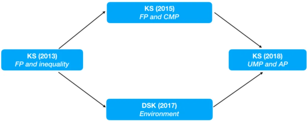
As already anticipated, we build upon the tradition of the “KS agent-based model”. In particular

with this work we unify the two branches of the model that both departed from the

Dosi et al.

(

2013

)

version. As a matter of fact in the following versions a bifurcation occurred (see figure

4

). On one

side

Dosi et al.

(

2015

) have embedded into the model a banking sector composed by heterogeneous

banks and have employed the model to study the effects of austerity fiscal policies and of interest

rate monetary policies; on the other side,

Lamperti et al.

(

2017

) appended an energy sector and a

climate box to the model in order to study the effects of climate shocks onto the economic system

as well as to investigate upon the feedbacks between environment and economy.

_{Here, we unify}

these two research strands and we introduce new policies exercises. In particular we focus on the

effects of balance sheet unconventional monetary policies – Quantitative Easing – and of accounting

policies – Mark-to-Market evaluation of banks assets. We do this with three objectives in mind: first,

to study and investigate whether the policy prescriptions of

Dosi et al.

(

2015

) are still valid when

an energy sector and a feedback mechanism between the economic system and the environment are

present; second, to introduce new unconventional policies that directly affect the balance sheets of

the banking sector (e.g. QE) and to study their relative performances vis-à-vis other policies that

bypass the banking system and provide direct monetary incentives for firms to invest and household

to consume (e.g. Helicopter Money); third, to draw and test new policy instruments that might

improve the environmental resilience (e.g. green-QE), minimizing the probability of climate shocks

to negatively affect the economy (this will come about in a follow-up paper).

For the sake of brevity, in what follows we do not describe the full model, which is however

in-cluded into appendix

A

, but we focus only on the newly introduced policies and on the modifications

of the original version of model that have been necessary to cope with the new policies. In particular,

the environmental section, the climate box, the energy sector, the technical change, the investment

behaviour of the firms and the consumption behaviour of the households are unchanged. Variations

to the credit market, to the balance sheets of the banking sector, to the government behaviour and

to the central bank behaviour have instead been necessary and constitute, together with the newly

15_{Also other two branchings took place, but moving from theDosi et al.(2010) version of the model. The first involved}

the study of labour market institutions and labour market policies (seeDosi et al.,2017a); the second involved the enlarge-ment of the model in a multinational dimension, allowing to investigate trade and catching up processes (seeDosi et al.,

Figure 4:

implemented policies the contribution of this paper.

4.1

Mark-to-Market accounting

As already mentioned in the introductory section, fair value accounting and historical value

account-ing are opposite extremes. Indeed, while the former looks at variations in the market value balance

sheet to indicate changes in the financial conditions of a bank, the latter looks at the realizations of

cash flows to measure changes the financial condition of the financial institution.

Since the

FASB

(

1991

) directives, the companies operating in the financial sector, are required

to report the fair value of the debt and equity securities that they hold in the asset sides of their

balance sheets. However, the usage of the mark-to-market principle implies that banks might be

forced to adjust the value of their assets account as soon as some of their direct borrowers default

on their loans during the year and even if these borrowers simply become more financially unstable.

This is true also for financial institutions holding government debt. If government bonds becomes

riskier, so that they cannot be considered as “risk-free assets” – a situation that has occurred during

the financial crisis and in the decade that followed it (see

Caballero et al.

,

2017

) – and if the

mark-to-market accounting principle is operating, the banks shall take the higher likelihood of default

of the government into account and accordingly, they shall adjust their asset by depreciating the

government bonds they have in their portfolio of assets.

In the previous versions of the model, this evaluation mechanism was absent and the unique

mechanism by which the value of the banking sector asset side could have declined, was generated

by the bankruptcy of some consumption good firms, then unable to repay their outstanding debt to

some specific bank. This new accounting policy is instead an important mechanism for the model,

indeed it unleashes a positive feedbacks between the government and the banking sectors: if the

government accumulates debt – which we assume is the metric for risk – then the government bonds

are revalued downward, because there is an higher chance that the government might go bankrupt.

This in turn, decreases the assets side of the banking system, reducing the availability of credit which,

might have a negative impact on the ability of producing new private investments. Also the opposite

holds true and if the public debt decreases (due to surpluses), bonds are revalued upward and this

allows banking industry to produce a larger amount of credit to the consumption good firms.

In particular we here model the mark to market accounting principle as an evaluation standard

that the banks adopt when filling and reporting their balance sheets. Such a standard requires that

the banks evaluation of the bonds in their portfolio is performed at their current price (market value)

rather than at their nominal historical value.

Let’s begin from the definition of the bonds market in the model. The variation in the bonds

supply is determined by the deficit. Whenever the government spending is larger than government

revenues, the government shall issue an amount of bonds equal to the amount of deficit. Quite

naturally, as time passes by, the total outstanding amount of bonds is equivalent to the government

debt. Hence, for every period we have that:

B

=

min

{

G

−

T

, 0

}

B

=

Debt

The demand for bonds instead derive from the liquidity situation of the banks. In particular,

we assume that the banks buy a quota of the total newly issued bonds (i.e. a quota of the deficit)

proportionally to their market share. This implies that:

B

=

f

∗

B

where f

represents the market share bought by the bank h in period t.

Liquidity of the banks is however important and plays a role. To demand such an amount of

government bonds indeed, the bank shall be sufficiently liquid and shall hold an equivalent amount

of cash to pay for the desired amount of newly issued bonds. Some banks might indeed from time

to time be illiquid and will not be able to buy the whole amount of government debt they desire.

In this case, a second mechanism that we introduce in this version of the model comes about: the

lender of last resort central bank. Here we indeed assume that the the Central Bank intervenes in the

primary market for bonds and directly buys the quota of newly issued bonds that is leftover due to

the insufficient liquidity of the banking system. Ideally this can be considered as a very mild form

of central bank unconventional monetary policy, even if the central bank in such occasions does not

affect the balance sheets of the financial institutions.

When the bonds market is closed and the quotas of newly issued bonds have been assigned,

government bonds are stored by the banks in the asset side of the balance sheet. From the following

period onward, they will be evaluated at their fair value which is determined as follows: we assume

that the discount factor by which the assets are reevaluated is a function of the government debt to

GDP – the implicit measure of the government solvency – and of the quota of total outstanding bonds

hold by the Central Bank – an implicit measure of the illiquidity of the credit market. In formula we

then have that. In particular, moving from a fixed baseline interest rate paid on government bonds

r

₌

_{¯r, the discount factor will evolve according to:}

r

=

r

+

v

Debt

GDP

+

v

∗

B

B

;

antic-ipated, positively depends on the likelihood of government insolvency and on the illiquidity of the

credit market.

Thus at the end of the period, when compiling the balance sheet, the fair value of the government

bonds is:

B

=

B

1

+

r

.

In section

5

we will report outcomes stemming from the comparison between scenarios in which

the mark-to-market accounting principle is used, against scenarios in which historical value is used.

In the second case, we will simply set r

=

0,

∀

t

∈ [

1, T

]

and hence all the banks will always

evaluate bonds at their nominal value B

discounted only at the baseline, risk-free, rate r

.

4.2

Quantitative Easing

Closely following the description of the implementation of QE by the 4 major central banks (see

section

2

), in the model we introduce a new policy instrument by which the central bank can directly

intervenes on the balance sheets of the financial institutions to dampen the effects of an illiquid credit

market.

In the K+S model, the first activity of the banking sector is that of providing credit to the

con-sumption good firms, whose internal financial resources are insufficient for investing into the new

(more efficient) machineries provided by the capital good firms as well as for covering production

costs. The credit activity endogenously generates a financial cycle (see

Dosi et al.

,

2015

). Some firms –

due to unsuccessful innovations and competitive losses – might become insolvent and go bankrupt.

When this happen, a direct negative effect on the bank with outstanding credit occurs: the loan

in-deed used to enter into the bank balance sheet as an asset, but when the borrower defaults, this asset

loses all its value – and it becomes a bad debt – causing a net loss for the bank, and in turn it

neg-atively affects the ability of the bank to inject new liquidity into the real sector, lowering the bank’s

credit supply.

While in the previous version of the model the bad debts generated an immediate net loss for the

bank, we assume that the QE dampens this situation as the cost is now shared between the bank itself

and the Central Bank, which intervenes by injecting cash into the banks balance sheet, and partially

contributing to the loss. In particular, we assume that Quantitative Easing takes a very simple linear

form:

QE

=

α

BadDebt

where QE

is the amount of resources that the central bank injects into the banks h balance

sheet to buy a fraction fraction α

∈ [

0, 1

]

of the bank h bad debts. Very intuitively, the parameter

α

represents a fine tuning parameter measuring the QE aggressiveness: the higher α

, the larger

the intervention of the central bank and the lower the effect that a possible bankruptcy might have

on the bank h credit supply. In practice, the Central Banks exogenously generates new liquidity,

and partially bears the cost of the banks loss. This mechanism might be of particular importance

to dampen the credit cycle and to avoid a shortage of credit supply. Indeed, in the K+S model, the

credit supply for each bank is positively related to its equity and is instead inversely dependent on

the amount of bad debt:

TC

=

NW

τ

(

1

+

βBadDebt

)

meaning that a QE intervention, aimed at reducing BadDebt shall support the total credit supply

toward the real sector of the economic system.

5

Results

The analysis of the model is performed by means of agent-based MonteCarlo simulations: we run

a set of independent simulations to wash away across-simulation variability and to evaluate the

statistical significance of our policy claims.

Before moving to the policy exercise, we verify that in the baseline case, the new version of the

model is able to replicate all the stylized facts already presented in the previous versions of the model,

to which we build upon. In particular, we replicate the full list of stylized facts presented in

Dosi et al.

(

2015

);

Lamperti et al.

(

2017

). While in table

1

we present some summary statistics under the baseline

scenario, the first validation test – i.e. replication of stylized fact – is presented in the appendix

B

.

After having observed the ability of the model of replicating a large list of stylized fact, we proceed

with the policy exercises.

The final aim of this paper is that of evaluating different mix of policies. Thanks to the flexibility of

the agent-based simulation framework we can compare the model under different policy scenarios.

In particular, as anticipated, we are interested into the evaluation of the effects of the Mark-to-Market

accounting policy as well as of the Quantitative Easing on the real sector of our simulated economic

system. Tables

2

and

3

summarize the results of the policy comparisons, reporting respectively

aver-ages and standard deviations – i.e. measuring respectively growth and volatility. The values in the

table report, for each variable, the ratio between the average value of a variable in the first scenario

(as specified in the "id" column) and the average value of that same variable in the second scenario.

We also report the t-statistics and the p-values aiming at statistically test whether the ratio between

16_{All the results presented below refer to averages across 50 MonteCarlo runs. Since most of the variables under}

investi-gation are ergodic (seeGuerini and Moneta,2017), 50 MonteCarlo runs, each composed by 500 time periods (and leading to 25000 observations for each variable) is sufficient to obtain reliable statistics. Between the different scenarios, the unique source of variation is given by the Pseudo Random Number Generator.

17_{We show that the model produces at the macro-level: (i) a self-sustained long-run endogenous growth with (ii) short}

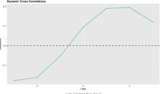
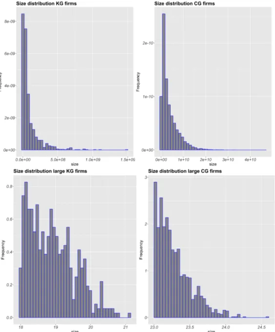
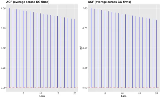
run business cycles, (iii) fat-tailed GDP growth rates distribution (iv) coherent volatility of GDP, consumption and invest-ment, (v) coherent dynamic auto- and cross-correlations between GDP, consumption and investinvest-ment, (vi) coherent dy-namic cross-correlations of private debt and total deposits with GDP, (vii) coherent dydy-namic auto- and cross-correlations between private debt and amount of bad debt, (viii) coherent dynamic cross-correlations of GDP and energy demand. At the micro level: (i) right-skewed fat-tailed distribution of firms size in both sectors, (ii) Pareto distribution of large firms in both sectors, (iii) Laplace distribution of the growth rates of firms in both sectors, (iv) non-persistent productivity growth rates of firms in both the sectors.

variable

MC average

MC std. dev.

1

GDP growth

0.0307

0.0006

2

GDP volatility

0.0378

0.0036

3

Crisis likelihood

0.0438

0.0129

4

Consumption growth

0.0307

0.0006

5

Consumption volatility

0.0236

0.0032

6

Investment growth

0.0303

0.0015

7

Investment volatility

0.4507

0.0535

8

Unemployment level

0.0325

0.0281

9

Full employment likelihood

0.0685

0.0936

10

Private debt growth

0.3384

0.0759

11

Private debt volatility

0.0017

0.0062

12

Energy demand growth

0.0265

0.0020

13

Emissions growth

0.0004

0.0003

14

Emissions in 2100

2.3827

0.1174

15

Temperature anomaly in 2100

3.1615

0.1694

Table 1:

the two considered scenarios, is significantly different from 1 (the null hypothesis according to which

the two compared scenario provide the same results).

5.1

Standalone policies

We begin by comparing the Mark-to-market (MtM) scenario with the baseline (Base) case (ID = 1

in tables

2

and

3

). The unique difference in the design of the model between these two scenarios is

given by the accounting policy, which impacts only on the balance sheets of the banks, affecting in

turn the aggregate credit supply and hence, the real sector. We observe that when the Mark-to-Market

is adopted, the growth rates of GDP and consumption are significantly lower and this in turn also

generates a higher levels of unemployment, which (via the subsidies that the government shall pay)

strongly impact on the public finances, generating much larger deficits and increasing Debt-to-GDP.

Similar results are also obtained when the MtM and the Baseline cases are compared under a

dual-mandate monetary policy (ID = 6 in the two tables). In such a situation indeed, also the investment

growth rate is significantly lower in the MtM scenario vis-à-vis the baseline one. Also concerning

the volatility of the system, presented in table

3

, we observe that for most of the considered variables

the standard deviation is higher in the MTM scenario with respect to the baseline one (see ID = 6 for

example). All in all therefore, we conclude that the standalone Mark-to-market accounting policy, is

worse off with respect to the historical value accounting practice. Furthermore, the MtM does not

even generate a trade-off between growth and volatility: in both the comparisons, the historical value

seems to be better-off.

The second standalone comparison that we perform concerns the exploratory evaluation of the

proposal of transforming the QE (an unconventional monetary policy tool) into a conventional

in-18_{The negative sign in front of the Debt-to-GDP value in Row 1 of table2(i.e. the−8.45) has to be interpreted as a shift}

from the government surplus (present on average in the baseline scenario) to a position of government debt (present on average in the Mark-to-Market scenario).

strument for the Central bank to use in its standard operations also in more tranquil periods (see

Quint and Rabanal

,

2017

). The outcomes of our simulation exercise (ID = 2 and ID = 7, respectively

for the comparisons in a pure inflation targeting scenario or in a dual mandate scenario) suggest

that the QE, adopted into the baseline scenario (in which the government is in surplus and inflation

and output growth are relatively stable) makes no harm, but also does not make any better for the

system. Average growth rates are statistically indistinguishable as well as volatilities.

This absence

of statistical difference might be due to the fact that in the baseline scenario the economy does not

experience prolonged and severe crises, therefore also the periods of high government deficit are rare

and low are the volume of bad debts; as a consequence, both the intervention of the Central Bank in

the bonds market as a lender of last resort and the amount of bad debt acquired by the Central banks

trough QE operations are relatively weak and scarce, explaining the low impact of the QE policy.

Hence, we conclude that there is no need of burdening a central bank with another discretional tool

for monetary policy: in tranquil periods, with historical cost accounting, the interest rate monetary

policy rules, accompanied by a countercyclical fiscal policy, are sufficient to avoid the generation of

large and prolonged crises.

5.2

Composition of policies

The second step for policy analysis is that of evaluating policy combinations. In particular we aim at

evaluating the performances of a scenario in which the QE monetary policy is employed together

with the MtM accounting policy. We observe that the role for the QE, when accompanied with

counter-cyclical fiscal policies, might be substantial. As a matter of fact, we can see (ID = 3 and

ID = 8) that when we compare a policy mix embedding the QE policy with the MtM accounting

framework with the Baseline one, the differences are small and mostly non statistically significant

(only the surplus deteriorates vis-à-vis the baseline case). This implies that the QE is able to offset

the negative effects brought about by the MtM accounting policy. The positive effect of the QE, can

also be observed (ID = 4, ID = 9) by comparing a policy scenario which includes both QE and MtM

against a scenario where there is MtM without unconventional monetary policy. We observe indeed

that the growth rates of GDP, consumption and investment are higher that the unity.

The keys to understand and interpret the transmission mechanism that are below this set of

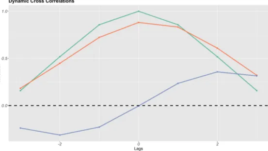
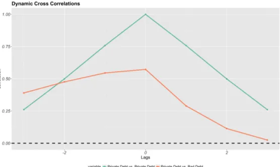
re-sults are in the existence of a positive feedback between GDP, private debt and bad debt which are

positively correlated at several lags and leads – we document the dynamic cross correlations between

these variables in appendix

B

, in figures

8

and

9

. The fair value accounting policy further increases

this positive correlation structure indeed: in periods of expansion, the higher GDP and the surplus

created by the government decrease the riskiness of government bonds. This in turn increases the

value of the bonds which are held as assets in the banks balance sheets, greasing the wheel of credit

that flows to the real sector. But a too large availability of credit, also implies that an higher fraction

of the loans will become bad-debts because of the failure of some consumption good firms that will

then be unable to repay the debt. Without the QE, this in turn reduces the availability of credit and

generate recessions. A boom and bust dynamic is endogenously generated by such a transmission

A VERAGES ID GDP gr owth Cons. gr owth Inv . gr owth Unemp. Inflation Debt-to-GDP Lar ge Crises 1 MTM / Base (ratio) 0.93 0.93 0.99 4.32 0.96 -8.45 1.11 1 MTM / Base (t-stat) -3.31 -3.28 -0.44 2.88 -1.42 -2.34 1.62 1 MTM / Base (p-value) 0.00 0.00 0.67 0.01 0.16 0.02 0.11 2 QE / Base (ratio) 1.00 1.00 1.01 1.17 0.99 0.79 0.98 2 QE / Base (t-stat) -0.72 -0.89 0.97 2.30 -0.69 -1.52 -0.25 2 QE / Base (p-value) 0.48 0.38 0.34 0.03 0.49 0.13 0.81 3 QE + MTM / Base (ratio) 1.00 0.99 1.00 1.14 0.99 0.64 1.10 3 QE + MTM / Base (t-stat) -1.41 -1.46 0.07 1.50 -0.30 -2.54 1.25 3 QE + MTM / Base (p-value) 0.16 0.15 0.94 0.14 0.76 0.01 0.22 4 QE + MTM / MTM (ratio) 1.10 1.10 1.01 0.97 1.06 0.76 1.04 4 QE + MTM / MTM (t-stat) 2.89 2.87 0.55 -0.31 1.96 -3.18 0.71 4 QE + MTM / MTM (p-value) 0.01 0.01 0.58 0.76 0.06 0.00 0.48 5 QE + MTM / QE (ratio) 1.00 1.00 0.99 1.04 1.01 1.10 1.26 5 QE + MTM / QE (t-stat) -0.49 -0.37 -0.90 0.57 0.71 0.70 3.18 5 QE + MTM / QE (p-value) 0.63 0.71 0.37 0.57 0.48 0.49 0.00 6 MTM + DM / Base + DM (ratio) 0.98 0.98 0.98 1.51 1.00 0.50 1.09 6 MTM + DM / Base + DM (t-stat) -1.87 -1.89 -2.21 1.51 -0.12 -1.15 1.06 6 MTM + DM / Base + DM (p-value) 0.07 0.07 0.03 0.14 0.90 0.25 0.30 7 QE + DM / Base + DM (ratio) 1.00 1.00 0.99 1.06 1.00 0.86 1.10 7 QE + DM / Base + DM (t-stat) -0.11 -0.09 -0.92 1.16 -0.16 -0.55 1.10 7 QE + DM / Base + DM (p-value) 0.91 0.93 0.36 0.25 0.87 0.59 0.28 8 QE + MTMT + DM / Base + DM (ratio) 1.00 1.00 1.00 1.10 0.99 0.90 1.14 8 QE + MTMT + DM / Base + DM (t-stat) 0.58 0.59 0.32 1.77 -0.66 -0.37 1.35 8 QE + MTMT + DM / Base + DM (p-value) 0.57 0.56 0.75 0.08 0.51 0.72 0.18 9 QE + MTMT + DM / MTM + DM (ratio) 1.02 1.02 1.02 1.04 1.00 1.10 1.13 9 QE + MTMT + DM / MTM + DM (t-stat) 1.97 2.00 2.35 0.74 -0.19 0.87 1.52 9 QE + MTMT + DM / MTM + DM (p-value) 0.05 0.05 0.02 0.46 0.85 0.39 0.13 10 QE + MTMT + DM / QE + DM (ratio) 1.00 1.00 1.02 1.07 0.99 1.18 1.14 10 QE + MTMT + DM / QE + DM (t-stat) 0.86 0.82 1.73 1.60 -0.40 1.46 1.58 10 QE + MTMT + DM / QE + DM (p-value) 0.39 0.41 0.09 0.12 0.69 0.15 0.12

T

able

2:

ST ANDARD DEVIA TIONS ID GDP gr owth Cons. gr owth Inv . gr owth Unemp. Inflation Deb t-to-GDP 1 MTM / Base (ratio) 1.04 1.11 1.02 2.42 1.06 20.60 1 MTM / Base (t-stat) 1.79 2.40 0.81 2.83 2.06 2.88 1 MTM / Base (p-value) 0.38 1.46 1.47 1.30 1.86 2.56 2 QE / Base (ratio) 0.98 1.01 1.00 1.05 0.99 1.20 2 QE / Base (t-stat) 0.08 0.02 0.42 0.01 0.05 0.01 2 QE / Base (p-value) 0.70 0.15 0.15 0.20 0.07 0.01 3 QE + MTM / Base (ratio) 1.00 1.02 1.01 1.05 1.01 1.37 3 QE + MTM / Base (t-stat) -1.04 0.31 -0.16 1.01 -0.62 1.58 3 QE + MTM / Base (p-value) 1.22 1.53 1.14 0.91 1.90 2.29 4 QE + MTM / MTM (ratio) 0.98 0.96 1.01 0.93 0.97 1.05 4 QE + MTM / Base (t-stat) 0.30 0.76 0.87 0.32 0.54 0.12 4 QE + MTM / Base (p-value) 0.23 0.13 0.26 0.37 0.06 0.03 5 QE + MTM / QE (ratio) 1.03 1.02 1.03 1.02 1.03 1.27 5 QE + MTM / QE (t-stat) 0.22 0.59 0.61 0.67 0.49 1.49 5 QE + MTM / QE (p-value) 0.92 1.89 0.94 2.07 1.70 2.27 6 MTM + DM / Base + DM (ratio) 0.99 1.02 1.01 1.42 1.01 2.52 6 MTM + DM / Base + DM (t-stat) 0.83 0.56 0.54 0.51 0.63 0.14 6 MTM + DM / Base + DM (p-value) 0.36 0.06 0.35 0.04 0.10 0.03 7 QE + DM / Base + DM (ratio) 1.00 1.01 1.02 1.00 1.02 1.16 7 QE + DM / Base + DM (t-stat) -1.39 -1.31 0.37 -0.98 -1.15 0.36 7 QE + DM / Base + DM (p-value) -3.40 0.67 -2.98 0.08 -2.97 6.91 8 QE + MTMT + DM / Base + DM (ratio) 1.01 1.04 1.04 1.06 1.05 1.24 8 QE + MTMT + DM / Base + DM (t-stat) 0.17 0.19 0.71 0.33 0.25 0.72 8 QE + MTMT + DM / Base + DM (p-value) 0.00 0.51 0.00 0.94 0.00 0.00 9 QE + MTMT + DM / MTM + DM (ratio) 1.02 1.03 1.03 1.04 1.05 1.25 9 QE + MTMT + DM / MTM + DM (t-stat) 2.01 0.89 1.38 0.29 1.70 1.66 9 QE + MTMT + DM / MTM + DM (p-value) -6.09 -1.02 -3.99 0.89 -4.71 2.13 10 QE + MTMT + DM / QE + DM (ratio) 1.01 1.04 1.02 1.07 1.04 1.22 10 QE + MTMT + DM / QE + DM (t-stat) 0.05 0.38 0.17 0.77 0.10 0.10 10 QE + MTMT + DM / QE + DM (p-value) 0.00 0.31 0.00 0.38 0.00 0.04

T

able

3:

mechanism. The QE instead is an asymmetric measure that introduces a negative feedback between

the dynamic cross-correlation between debt and bad-debt: by cleaning the banks balance sheet and

removing bad-debts the QE avoids large falls in the credit supply even in recession periods,

support-ing investments. The QE basically, works as a reflectsupport-ing barrier that pushes the economic system far

from the recessions in a relatively short term.

6

Conclusions

Accounting policies have been largely neglected by the economic literature during the last decades,

notwithstanding the important macroeconomic and financial implications that they might have.

However, as also happened in the past, large financial and economic crises led to a

reconsidera-tion of accounting policies. As a matter of fact, after the advent of the great financial crisis, some

economists such as

Bignon et al.

(

2009

);

Kolasinski

(

2011

) have begun to criticize the status quo of

the accounting standards: the fair value or mark-to-market principle. In this paper we carry on such

a debate, and we add to the empirical research by investigating by means of a new version of the

large scale KS agent-based model (following the lines of

Dosi et al.

,

2010

,

2013

,

2015

;

Lamperti et al.

,

2017

) the effects of the mark-to-market policy. Furthermore, since the reply of most central banks to

the turmoils of the 2008 crisis have been unconventional, we link the adoption of such accounting

standards with the introduction of innovative forms of monetary policies such as the Quantitative

Easing.

Fair value accounting is introduced by means of a periodic revision of the evaluation of the

bal-ance sheets of the banking industry, which is updated according to the risk of the balbal-ance sheet itself.

In particular, we introduce a negative correlation between government solvency and liquidity risks

and bonds value. Quantitative easing is instead introduced according to a close description of the

policies employed by the four major central banks. The central bank in our model indeed acquires

low valued assets and non-performing loans from the balance sheets of the banks, cleaning them up

and solving at the same time both liquidity and solvency of the banking industry, in turn

support-ing the credit activity and the degrees of investments. All in all therefore, with this paper we study

the macroeconomic and financial outcomes that emerge from the interactions between accounting

policies and unconventional monetary policies.

The policy results are in line with the intuitions by

Bignon et al.

(

2009

);

Heaton et al.

(

2010

) and

suggest that the fair value is possibly harmful, largely at odds with the objectives of long-run

sus-tainable growth: by increasing the relationship between loans (hence private debt), GDP and

non-performing loans, the mark-to-market accounting practice leads to an higher likelihood of recessions

and to lower growth regimes. The QE policy, can counterbalance these negative effects and can

re-store long-term economic growth: hence it is welcome in a context where the fair-value is the rule.

However, QE alone does not perform better-off than a standard interest rate monetary policy,

accom-panied by counter-cyclical fiscal policy, aimed at supporting the consumption levels of unemployed

workers.

Acknowledgments

We thank Marc Lavoie and Stefano Battiston as well as the participants of the 2017 EAEPE Conference and of the 2018 FINEXUS workshop for useful comments and suggestions. GD, MG, MN, AR, TT acknowledge financial support of the European Union Horizon 2020 research and innovation programme under grant agree-ments No. 649186 (ISIGrowth) as well as the financial support of the Horizon 2020 Framework Program of the European Union under the grant agreement No. 640772 - Project DOLFINS (Distributed Global Financial Sys-tems for Society). FL acknowledges financial support from EU-FP7 project IMPRESSIONS under grant No 603416.