Clustering in Complex Directed Networks

Clustering in complex directed networks

Giorgio Fagiolo*

Sant’Anna School of Advanced Studies, Laboratory of Economics and Management, Piazza Martiri della Libertà 33, I-56127 Pisa, Italy 共Received 6 February 2007; published 16 August 2007兲

Many empirical networks display an inherent tendency to cluster, i.e., to form circles of connected nodes. This feature is typically measured by the clustering coefficient共CC兲. The CC, originally introduced for binary, undirected graphs, has been recently generalized to weighted, undirected networks. Here we extend the CC to the case of共binary and weighted兲 directed networks and we compute its expected value for random graphs. We distinguish between CCs that count all directed triangles in the graph共independently of the direction of their edges兲 and CCs that only consider particular types of directed triangles 共e.g., cycles兲. The main concepts are illustrated by employing empirical data on world-trade flows.

DOI:10.1103/PhysRevE.76.026107 PACS number共s兲: 89.75.⫺k, 89.65.Gh, 87.23.Ge, 05.70.Ln

Networked structures emerge almost ubiquitously in com-plex systems. Examples include the Internet and the WWW, airline connections, scientific collaborations and citations, trade and labor-market contacts, friendship and other social relationships, business relations and research and develop-ment partnerships, cellular, ecological, and neural networks 关1–3兴.

The majority of such “real-world” networks have been shown to display structural properties that are neither those of a random graph关4兴, nor those of regular lattices. For

ex-ample, many empirically observed networks are small worlds关5,6兴. These networks are simultaneously

character-ized by two features关7兴. First, as happens for random graphs,

their diameter 关8兴 increases only logarithmically with the

number of nodes. This means that, even if the network is very large, any two seemingly unrelated nodes can reach each other in a few steps. Second, as happens in lattices, small-world networks are highly clustered, i.e., any two neighbors of a given node have a probability of being them-selves neighbors which is much larger than in random graphs.

Network clustering is a well-known concept in sociology, where notions such as “cliques” and “transitive triads” have been widely employed关9,10兴. For example, friendship

net-works are typically highly clustered共i.e., they display high cliquishness兲 because any two friends of a person are very likely to be friends.

The tendency of a network to form tightly connected neighborhoods共more than in the random uncorrelated case兲 can be measured by the clustering coefficient 共CC兲, see 关11,12兴. The idea is very simple. Consider a binary,

undi-rected network 共BUN兲 described by the graph G=共N,A兲, where N is the number of the nodes and A =兵aij其 is the N ⫻N adjacency matrix, whose generic element aij= 1 if and only if there is an edge connecting nodes i and j共i.e., if they are neighbors兲 and zero otherwise. Since the network is un-directed, A is symmetric关13兴. For any given node i, let dibe its degree, i.e., the number of i’s neighbors. The extent to which i’s neighborhood is clustered can be measured by the percentage of pairs of i’s neighbors that are themselves

neighbors, i.e., by the ratio between the number of triangles in the graph G with i as one vertex 共labeled as ti兲 and the number of all possible triangles that i could have formed 关that is, Ti= di共di− 1兲/2兴 关14兴. It is easy to see that the CC for node i in this case reads

Ci共A兲 = 1 2

兺

兺

where 共A3兲ii is the ith element of the main diagonal of A3 = A A A. Each product aijaihajh is meant to count whether a triangle exists or not around i. Notice that the order of sub-scripts is irrelevant, as all entries in A are symmetric. Of course, Ci僆关0,1兴. The overall 共network-wide兲 CC for the graph G is then obtained by averaging Ciover the N nodes, i.e., C = N−1兺_i=1N Ci. In the case of a random graph where each link is in place with probability p僆共0,1兲, one has that E关C兴=p 共E stands for the expectation operator兲.

Binary networks treat all edges present in G as they were completely homogeneous. More recently, scholars have be-come increasingly aware of the fact that real networks ex-hibit a relevant heterogeneity in the capacity and intensity of their connections 关15–20兴. Allowing for this heterogeneity

might be crucial to better understand the architecture of com-plex networks. In order to incorporate such a previously ne-glected feature, each edge ij present in G共i.e., such that aij = 1兲 is assigned a value wij⬎0 proportional to the weight of that link in the network. For example, weights can account for the amount of trade volumes exchanged between coun-tries共as a fraction of their gross domestic product兲, the num-ber of passengers traveling between airports, the traffic be-tween two Internet nodes, the number of emails exchanged between pairs of individuals, etc. Without loss of generality, we can suppose that wij僆关0,1兴 关21兴. A weighted undirected network共WUN兲 is thus characterized by its N⫻N symmetric weight matrix W =兵wij其, where wii= 0, all i. Many network measures developed for BUNs have a direct counterpart in WUNs. For example, the concept of node degree can be replaced by that of node strength关15兴:

si=

兺

wij. 共2兲

For more complicated measures, however, extensions to WUNs are not straightforward. To generalize the CC of node i to WUNs, one has indeed to take into account the weight associated to edges in the neighborhood of i. There are many ways to do that关22兴. For example, suppose that a triangle ihj

is in place. One might then consider only weights of the edges ih and ij 关15兴. Alternatively, one might employ the

weights of all the edges in the triangle. In turn, the total contribution of a triangle can be defined as the geometric mean of its weights 关23兴 or simply as the product among

them关24–27兴. In what follows, we will focus on the

exten-sion of the CC to WUNs originally introduced in关23兴:

C ˜ i共W兲 = 共1/2兲

兺

兺

the measure C˜i ranges in 关0,1兴 and reduces to Ci when weights become binary. Furthermore, it takes into account weights of all edges in a triangle 共but does not consider weights not participating in any triangle兲 and is invariant to weight permutation for one triangle. Notice that C˜i= 1 only if the neighborhood of i actually contains all possible triangles that can be formed and each edge participating in these tri-angles has unit共maximum兲 weight. Again, one can define the overall clustering coefficient for WUNs as C˜ =N−1_兺

i=1 N

C ˜

i. In this paper we discuss extensions of the CC for BUNs and WUNs 关Eqs. 共1兲 and 共3兲兴 to the case of directed

works. It is well known that many real-world complex net-works involve nonmutual relationships, which imply non-symmetric adjacency or weight matrices. For instance, trade volumes between countries关28–30兴 are implicitly directional

relations, as the export from country i to country j is typi-cally different from the export from country j to country i 共i.e., imports of i from j兲. If such networks are symmetrized 共e.g., by averaging imports and exports of country i兲, one could possibly underestimate important aspects of their net-work architecture.

Alternative extensions of the CC to weighted or directed networks have been recently introduced in the literature on “network motifs” 关31兴. As mentioned, 关23兴 generalizes the

CC to weighted—and possibly directed—networks. Simi-larly,关32兴 computes the recurrence of all types of three-node

connected subgraphs in a variety of real-world binary di-rected networks from biochemistry, neurobiology, ecology, and engineering. However, the weighted CC in关23兴 does not

explicitly discriminate between different directed triangles 共cf. Fig.1兲, while 关32兴 does not allow for a weighted

analy-sis. This work attempts to bridge the two latter approaches and presents a unifying framework where, in addition to the measures already discussed in关23,32兴, one is able to 共i兲

ex-plicitly account for directed and weighted links; and共ii兲 de-fine a weighted, directed version of the CC for any type of triangle pattern 共i.e., three-node connected subgraph兲. To compute such coefficients, we shall employ the actual and

potential number of directed-triangle patterns of any given type.

Preliminaries. In directed networks, edges are oriented and neighboring relations are not necessarily symmetric. In the case of binary directed networks共BDNs兲, we define the in-degree of node i as the number of edges pointing towards i共i.e., inward edges兲. The out-degree of node i is accordingly defined as the number of edges originating from i共i.e., out-ward edges兲. Formally,

di in =

兺

兺

where AT_{is the transpose of A,共A兲}

istands for the ith row of

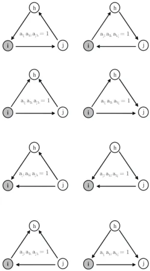
A, and 1 is the N-dimensional column vector 共1,1, ... ,1兲T_. The total degree of a node is simply the sum of its in- and out-degree: i j h a a a = 1 i j h a a a = 1 i j h a a a = 1 i j h a a a = 1 i j h a a a = 1 i j h a a a = 1 i j h a a a = 1 i j h a a a = 1

FIG. 1. Binary directed graphs. All eight different triangles with node i as one vertex. Within each triangle is reported the product of the form a_ⴱⴱa_ⴱⴱa_ⴱⴱ that works as indicator of that triangle in the network.

di tot = di in + di out =共AT+ A兲i1. 共6兲 Finally, provided that no self-interactions are present, the number of bilateral edges between i and its neighbors共i.e., the number of nodes j for which both an edge i→ j and an edge j→i exist兲 is computed as

di↔=

兺

aijaji= Aii2. 共7兲 It is easy to see that in BUNs one has di= di

tot − di↔.

The above measures can be easily extended to weighted directed networks 共WDNs兲, by considering in-, out-, and total-strength关see Eq. 共2兲兴.

Binary directed networks. We begin by introducing the most general extension of the CC to BDNs, which considers all possible directed triangles formed by each node, no mat-ter the directions of their edges. Consider node i. When edges are directed, i can generate up to eight different tri-angles with any pair of neighbors关33兴. Any product of the

form aijaihajh captures one particular triangle, see Fig.1for an illustration.

The CC for node i共C_iD兲 in BDNs can be thus defined 共like in BUNs兲 as the ratio between all directed triangles actually formed by i共ti

D_{兲 and the number of all possible triangles that}

i could form共Ti D_{兲. Therefore} Ci D_{共A兲 =} ti D Ti D=

共1/2兲

兺

兺

where 共also in what follows兲 sums span over j⫽i and h ⫽共i, j兲. In the first line of Eq. 共8兲, the numerator of the

fraction is equal to ti D

, as it simply counts all possible prod-ucts of the form aijaihajh 共cf. Fig. 1兲. To see that Ti

D = di tot_共d i tot_{− 1兲−2d} i

↔_{, notice that i can be possibly linked to a} maximum of di

tot_共d i

tot_{− 1兲/2 pairs of neighbors and with each} pair can form up to two triangles共as the edge between them can be oriented in two ways兲. This leaves us with di

tot_共d i tot − 1兲 triangles. However, this number also counts “false” tri-angles formed by i and by a pair of directed edges pointing to the same node, e.g., i→ j and j→i. There are d_i↔of such occurrences for node i, and for each of them we have wrongly counted two “false” triangles. Therefore by sub-tracting 2d_i↔from the above number we get Ti

D

. This implies that Ci

D_{僆关0,1兴. The overall CC for BDNs is defined as C}D = N−1_兺 i=1 N Ci D .

The CC in Eq.共8兲 has two nice properties. First, if A is

symmetric, then Ci D_共A兲=C

i共A兲, i.e., it reduces to Eq. 共1兲 when networks are undirected. To see this, note that if A is symmetric then d_itot= 2diand di↔= di. Hence

Ci D_{共A兲 =} 共2A兲ii 3 2关2di共2di− 1兲 − 2di兴 = 共A兲ii 3 di共di− 1兲 = Ci共A兲. 共9兲 Second, the expected value of C_iD in random graphs, where each edge is independently in place with probability p僆共0,1兲 关i.e., aijare i.i.d. Bernoulli共p兲 random variables兴,

is still p共as happens for BUNs兲. Indeed, the expected value of ti

D _{is simply 4共N−1兲共N−2兲p}3_{. Furthermore, note that d} i in ⬃di

out_{⬃bin共N−1,p兲 and d} i

tot_{⬃bin(2共N−1兲,p). Hence}

E关d_itot共d_itot− 1兲兴=E关d_itot兴2_{− E关d} i

tot_{兴=2共N−1兲共2N−3兲p}2_. Simi-larly, E关di↔兴=共N−1兲p2, which implies that E关Ti

D_{兴=4共N−1兲} ⫻共N−2兲p2_{and finally that E关C}

i D_兴=p.

Weighted directed networks. The CC for BDNs defined above can be easily extended to weighted graphs by replac-ing the number of directed triangles actually formed by i共ti

D_兲 with its weighted counterpart t˜_iD. Given Eq. 共3兲, t˜_iD can be thus computed by substituting A with W关1/3兴. Hence

C˜i D_{共W兲 =} t˜i D Ti D= 关W关1/3兴_+共WT_{兲关1/3兴兴} ii 3 2关di tot_共d i tot_{− 1兲 − 2d} i ↔_兴. 共10兲 Note that when the graph is binary 共W=A兲, then 共W兲关1/3兴 = W = A. Hence C˜_iD共A兲=C_iD共A兲. Moreover, if W is a symmet-ric weight matrix, then the numerator of C˜_iD共W兲 becomes 关2W关1/3兴_兴3_{. By combining this result with the denominator in} Eq. 共9兲, one has that C˜i

D_共W兲=C˜

i共W兲 for any symmetric W 关34兴.

To compute expected values of C˜i D

in random graphs, sup-pose that weights are drawn using the following two-step algorithm. First, assume that any directed edge i→ j is in place with probability p 共independently across all possible directed edges兲. Second, let the weight wij of any existing directed edge共i.e., in place after the first step兲 be drawn from an independent random variable uniformly distributed over 共0,1兴 关35兴. In this case, one has that E关wij兴1/3=

3p

4. It easily follows that for this class of random weighted graphs:

E关C˜i D_{兴 = E关C˜} i兴 =

冉

冊

The overall CC for WDN is again defined as C˜D = N−1_兺 i=1 N C ˜ i D .

Clustering and patterns of directed triangles. The CCs for BDNs and WDNs defined above treat all possible directed triangles as they were the same, i.e., if directions were irrel-evant. In other words, both CDand C˜Doperate a symmetri-zation of the underlying directed graph in such a way that the original asymmetric adjacency共respectively, weight兲 matrix A 共respectively, W兲 is replaced by the symmetric matrix A + AT 关respectively, W关1/3兴+共WT兲关1/3兴兴. This means that in the transformed graph, all directed edges are now bilateral. Fur-thermore, in binary 共respectively, weighted兲 graphs, edges that were already bilateral count as two共respectively, receive a weight equal to the sum of the weights of the two directed edges raised to 1/3兲.

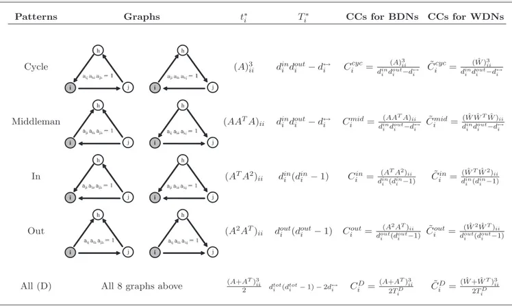
However, in directed graphs, triangles with edges pointing in different directions have a completely different interpreta-tion in terms of the resulting flow pattern. To put it differ-ently, they account for different network motifs. Looking again at Fig.1, it is possible to single out four patterns of directed triangles from i’s perspective. These are 共i兲 cycle, when there exists a cyclical relation among i and any two of its neighbors 共i→ j→h→i, or vice versa兲; 共ii兲 middleman,

when one of i’s neighbors共say j兲 both holds an outward edge to a third neighbor共say h兲 and uses i as a medium to reach h in two steps关36兴; 共iii兲 in, where i holds two inward edges;

and共iv兲 out, where i holds two outward edges.

When one is interested in measuring clustering in directed networks, it is important to separately account for each of the above patterns. This can be done by building a CC for each pattern 共in both BDNs and WDNs兲. As usual, each CC is defined as the ratio between the number of triangles of that pattern actually formed by i and the total number of triangles of that pattern that i can possibly form. Each CC will then convey information about clustering of each different pattern within tightly connected directed neighborhoods. In order to do that, we recall that the maximum number of all possible directed triangles that i can form 共irrespective of their pat-tern兲 can be decomposed as

Ti D = di tot_共d i tot_{− 1兲 − 2d} i ↔ =关di in di out − di↔兴 + 关di in di out − di↔兴 + 关di in_共d i in_{− 1兲兴} +关di out_共d i out_{− 1兲兴 = T} 1 D + T₂D+ T₃D+ T₄D. 共12兲 Let兵Ti cyc , Ti mid , Ti in , Ti

out_{其 be the maximum number of cycles,} middlemen, ins, and outs that i can form. Inspection suggests that Ti cyc = T₁D, Ti mid = T₂D, Ti in = T₃D, and Ti out = T₄D. To see why, consider, for example, Ti

cyc

. In that pattern type共see Fig. 1, top panels兲, node i is characterized by one inward link and one outward link. The maximum number of such patterns is given by di

in

di out

. Again, this also counts “false” triangles, formed by i and by a pair of directed edges pointing to and from a same node j. Therefore one has to subtract d_i↔to get Ti

cyc

. Incidentally, notice that Ti cyc

= Ti mid

. The reason why this is indeed the case becomes evident when one compares the top and the bottom pairs of triangle patterns in Fig. 1. In-deed, cycles and middlemen only differ from the orientation of the link connecting the partners of the reference node共i兲, which does not affect the maximum number of triangles that i can form.

In order to count all actual triangles formed by i, we no-tice that

ti D

=共A + AT兲ii=共A3兲ii+共AATA兲ii+共ATA2兲ii+共A2AT兲ii = t₁D+ t₂D+ t₃D+ t₄D. 共13兲 By letting兵ti cyc , ti mid , ti in , ti

out_{其 be the actual number of cycles,}

middlemen, ins, and outs formed by i, simple algebra reveals that t_icyc= t₁D, t_imid= t₂D, t_iin= t₃D, and t_iout= t₄D. For example,

ti cyc =1 2

兺

兺

A共i兲= A_共i兲AA共i兲= A_共ii兲3 . 共14兲 Similarly, ti mid =1 2

兺

兺

A共AT兲共i兲+ A_共i兲ATA共i兲兴 = A_共i兲ATA共i兲=共AATA兲_共ii兲. 共15兲 Notice that although Ti

cyc = Ti mid , now ti cyc_⫽t i mid as long as A is asymmetric.

Summing up, we can define a CC for each pattern as follows: Ciⴱ= tiⴱ Tiⴱ , 共16兲 where兵ⴱ其=兵cyc,mid,in,out其.

In the case of weighted networks, it is straightforward to replace tiⴱ with its weighted counterpart t˜iⴱ, where the adja-cency matrix A has been replaced by W关1/3兴. We then accord-ingly define C ˜ i ⴱ₌ t˜iⴱ Tiⴱ , 共17兲

where兵ⴱ其=兵cyc,mid,in,out其. To summarize the above dis-cussion, we report in Table I a taxonomy of all possible triangles with related measures for BDNs and WDNs.

Two remarks on Eqs.共16兲 and 共17兲 are in order. First, note

that, for 兵ⴱ其=兵cyc,mid,in,out其, 共i兲 when A is symmetric, Ciⴱ= Ci;共ii兲 when W is binary, C˜iⴱ= Ciⴱ;共iii兲 when W is sym-metric, C˜_iⴱ= C˜i. Second, in random graphs one still has that

E关Ciⴱ兴=p and E关C˜iⴱ兴=

共

兲

3 p.

Finally, network-wide clustering coefficients Cⴱ and C˜ⴱ can be built for any triangle pattern 兵cyc,mid,in,out其 by averaging individual coefficients over the N nodes.

These aggregate coefficients can be employed to compare the relevance of, say, cyclelike clustering among different networks, but not to assess the relative importance of cycle-like and middlemencycle-like clustering within a single network. In order to perform within-network comparisons, one can instead compute the fraction of all triangles that belong to the pattern兵ⴱ其僆兵cyc,mid,in,out其 in i’s neighborhood, that is, fiⴱ= tiⴱ ti D, f˜iⴱ= t˜iⴱ t˜i D, 共18兲

and then averaging them out over all nodes. Since for 兵ⴱ其僆兵cyc,mid,in,out其 we have that 兺_ⴱfiⴱ= 1 and 兺ⴱf˜iⴱ= 1, the above coefficients can be used to measure the contribu-tion of each single pattern to the overall clustering coeffi-cient. Notice that, in the case of BDNs, fiⴱcoefficients simply recover the recurrence of each pattern in the network, as computed in关32兴.

Empirical application. The above concepts can be mean-ingfully illustrated in the case of the empirical network de-scribing world trade among countries共i.e., the “world trade network,” WTN in what follows兲. Source data are provided by关37兴 and records, for any given year, imports and exports

from and to a large sample of countries共all figures are ex-pressed in current U.S. dollars兲. Here, for the sake of expo-sition, we focus on the year 2000 only关38兴. We choose to

build an edge between any two countries in the WTN if there is a nonzero trade between them and we assume that edge directions follow the flow of commodities. Let xijbe i’s ex-ports to country j and mjibe imports of j from i. In principle,

xij= mji. Unfortunately, due to measurement problems, this is not the case in the database. In order to minimize this

prob-lem, we will focus here on “adjusted exports” defined as eij=共xij+ mji兲/2 and we build a directed edge from country i to country j if and only if country i’s adjusted exports to country j are positive. Thus the generic entry of the adja-cency matrix aij is equal to 1 if and only if eij⬎0 共and 0 otherwise兲. Notice that, in general, eij⫽eji. In order to weight edges, adjusted exports can be tentatively employed. However, exporting levels are trivially correlated with the “size” of exporting and importing countries, as measured,

TABLE I. A taxonomy of the patterns of directed triangles and their associated clustering coefficients. For each pattern, we show the graph associated to it, the expression that counts how many triangles of that pattern are actually present in the neighborhood of i共t_iⴱ兲, the maximum number of such triangles that i can form共T_iⴱ兲, for ⴱ=兵cyc,mid,in,out,D其, and the associated clustering coefficients for BDNs and WDNs. Note that in the last column Wˆ =W关1/3兴=兵w_ij1/3其.

Patterns Graphs t∗i Ti∗ CCs for BDNs CCs for WDNs

Cycle i j h i j h (A)3ii dini douti − d↔i C cyc i = (A)3 ii din_i dout_i −d↔_i ˜ Cicyc= ( ˆW )3_ii din_i dout_i −d↔_i Middleman i j h i j h (AAT_A) ii dini douti − d↔i Cimid= (AAT_A)ii din_i dout_i −d↔_i ˜ Cmid i = ( ˆW ˆWTW )ˆ ii din_i dout_i −d↔_i In i j h i j h (AT_A2₎ ii dini (dini − 1) Ciin= (AT_A2_)ii din_i (din_i −1) ˜ Cin i = ( ˆWTWˆ2)ii din_i (din_i −1) Out i j h i j h (A2AT₎

ii douti (douti − 1) Ciout=

(A2_AT_)ii dout_i (dout i −1) ˜ Cout i = ( ˆW2WˆT)ii dout_i (dout i −1)

All (D) All 8 graphs above (A+AT)3ii

2 dtot_i (dtot i − 1) − 2d↔i CiD= (A+AT₎3 ii 2TD i ˜ CD i = ( ˆW + ˆWT)3_ii 2TD i 0 50 100 150 200 0 50 100 150 200 In−Degree O ut−Degree

FIG. 2. WTN: In- vs out-degree in the binary case. Axes are in log10scale. 101 102 103 10−0.2 10−0.1 100 Total Degree Overall CC

FIG. 3. WTN: Overall directed clustering coefficient vs total-degree in the binary case. Axes are in log10scale.

e.g., by their gross domestic products共GDPs兲. To avoid such a problem, we first assign each existing edge a weight equal to w˜ij= eij/ GDPi, where GDPiis country i’s GDP expressed in 2000 U.S. dollars. Second, we define the actual weight matrix as W =兵wij其 = w ˜ij max_h,k=1N 兵w˜hk其 , 共19兲

to have weights in the unit interval. Each entry wij tells us the extent to which country i共as a seller兲 depends on j 共as a buyer兲. The out-strength of country i 共i.e., i’s exports-to-GDP ratio兲 will then measure how i 共as a seller兲 depends on the rest of the world共as a buyer兲. Similarly, in-strengths denote how dependent is the rest of the world on i共as a buyer兲 关39兴.

The resulting WTN comprises N = 187 nodes/countries and 20 105 directed edges. The density is therefore very high 共␦= 0.5780兲. As expected, the binary WTN is substantially symmetric: there is a 0.9978 correlation关40兴 between in- and

out-degree共see Fig.2兲 and the 共nonscaled兲 S measure

intro-duced in关41兴 is close to zero 共0.003 97兲, indicating that the

underlying binary graph is almost undirected.

Thus, in the binary case, there seems to be no value added in performing a directed analysis: since A is almost symmet-ric, we should not detect any significant differences among clustering measures for our four directed triangle patterns. Indeed, we find that CD= 0.8125, while Ccyc= 0.8123, Cmid = 0.8127, Cin= 0.8142, Cout= 0.8108 关42兴. The fact that CD

⬎␦ also indicates that the binary 共directed兲 WTN is more clustered than it would be if it were random 共with density

␦= 0.5780兲. Finally, Fig 3 shows that individual CCs 共Ci D_兲 are negatively correlated with total degree共di

tot_{兲, the} correla-tion coefficient being −0.4102. This implies that countries with few 共respectively, many兲 partners tend to form very 共respectively, poorly兲 connected clusters of trade relation-ships.

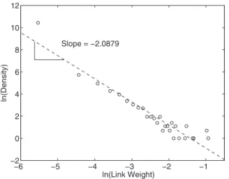
The binary network does not take into account the hetero-geneity of export flows carried by edges in the WTN. Indeed, when one performs a WDN analysis on the WTN, the picture changes completely. To begin with, note that weights wijare on average very weak 共0.0009兲 but quite heterogeneous 共weight standard deviation is 0.0073兲. In fact, weight distri-bution is very skewed and displays a characteristic power-law shape共see Fig.4兲 with a slope around −2.

−6 −5 −4 −3 −2 −1 −2 0 2 4 6 8 10 12 ln(Link Weight) ln(Density) Slope = −2.0879

FIG. 4. WTN: Log-log plot of the weight distribution.

10−4 10−2 100 10−3 10−2 10−1 100 In−Strength Out−Strength

FIG. 5. WTN: In-strength vs out-strength. Axes are in log₁₀ scale. 10−2 10−1 100 101 10−4 10−3 10−2 Total Strength O verall CC

FIG. 6. WTN: Overall CC vs total strength in the WDN case. Axes are in log10scale.

101 102 103 10−4 10−3 10−2 Total Degree O verall CC

FIG. 7. WTN: Overall CC vs total degree in the WDN case. Axes are in log10scale.

The matrix W is now weakly asymmetric. As Fig. 5

shows, in- and out-strengths are almost not correlated: the correlation coefficient is 0.09 共not significantly different from zero兲. Nevertheless, the 共not-scaled兲 S measure is still very low 共0.1118兲, suggesting that an undirected analysis would still be appropriate. We will see now that, even in this borderline case, a weighted directed analysis of CCs pro-vides a picture which is much more precise than共and some-times at odds with兲 that emerging in the binary case.

First, unlike in the binary case, the overall average CC 共C˜D_{兲 is now very low 共0.0007兲 and significantly smaller than} its expected value共0.2438兲 in random graphs 共with the same density ␦= 0.5780, but independently, uniformly distributed weights兲. Notice, however, that C˜D _{is almost equal to its} expected value in directed graphs characterized by the same topology共as defined by the adjacency matrix A兲 but the same weight distribution 共as defined by the nonzero elements in W兲, which turns out to be equal to 0.0005 共with a standard deviation of 0.0001兲 关43兴.

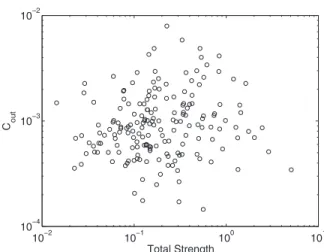
Second, C˜i D

is now positively correlated with total strength 共the correlation coefficient is 0.6421兲, cf. Fig. 6. This means that, when weight heterogeneity is taken into account, the implication we have drawn in the binary case is reversed: countries that are more strongly connected tend to form more strongly connected trade circles. Indeed, C˜i

D ex-hibits an almost null correlation with total degree, see Fig.7. Third, despite that the weighted network is only weakly asymmetric, there is a substantial difference in the way clus-tering is coupled with exports and imports. C˜i

D

is almost uncorrelated with in-strength共Fig.8兲, while a positive slope

is still in place when C˜_iD is plotted against out-strength. Hence the low clustering level of weakly connected coun-tries seems to depend mainly on their weakly exporting re-lationships.

Fourth, weighted CC coefficients associated to different triangle patterns now show a relevant heterogeneity: C˜ⴱ range from 0.0004 共cycles兲 to 0.0013 共out兲. In addition, cycles only account for 18% of all triangles, while the other three patterns account for about 27% each. Therefore coun-tries tend to form less frequently trade cycles, possibly be-cause they involve economic redundancies.

Finally, CCs for different triangle patterns correlate with strength measures in different ways. While C˜i

cyc , C˜i mid , and C ˜ i in

are positive and strongly correlated with total strength, C

˜

i out

is not; see Fig. 9: countries tend to maintain exporting relationships with connected pairs of partners independently of the total strength of their trade circles.

Concluding remarks. In this paper, we have extended the clustering coefficient 共CC兲, originally proposed for binary and weighted undirected graphs, to directed networks. We have introduced different versions of the CC for both binary and weighted networks. These coefficients count the number of triangles in the neighborhood of any node independently of their actual pattern of directed edges. In order to take edge directionality fully into account, we have defined specific CCs for each particular directed triangle pattern 共cycles, middlemen, ins, and outs兲. For any CC, we have also pro-vided its expected value in random graphs. Finally, we have illustrated the use of directed CCs by employing world trade network共WTN兲 data. Our exercises show that directed CCs can describe the main clustering features of the underlying WTN’s architecture much better than their undirected coun-terparts.

Thanks to Javier Reyes, Stefano Schiavo, and an anony-mous referee, for their helpful comments.

10−6 10−4 10−2 100 102 10−4 10−3 10−2 In−Strength O verall CC

FIG. 8. WTN: Overall CC vs in-strength in the WDN case. Axes are in log10scale.

10−2 10−1 100 101 10−4 10−3 10−2 Total Strength Cout

FIG. 9. WTN: C˜_ioutvs total strength in the WDN case. Axes are in log₁₀scale.

关1兴 R. Albert and A. Barabási, Rev. Mod. Phys. 74, 47 共2002兲. 关2兴 M. Newman, SIAM Rev. 45, 167 共2003兲.

关3兴 S. Dorogovtsev and J. Mendes, Evolution of Networks: From Biological Nets to the Internet and WWW共Oxford University Press, Oxford, 2003兲.

关4兴 B. Bollobás, Random Graphs 共Academic Press, New York, 1985兲.

关5兴 The Small World, edited by M. Kochen 共Ablex, Norwood, 1989兲.

关6兴 D. Watts, Small Worlds 共Princeton University Press, Princeton, 1999兲.

关7兴 L. Amaral, A. Scala, M. Barthélemy, and H. Stanley, Proc. Natl. Acad. Sci. U.S.A. 97, 11149共2000兲.

关8兴 As computed by the average shortest distance between any two nodes关44兴.

关9兴 S. Wasserman and K. Faust, Social Network Analysis. Methods and Applications 共Cambridge University Press, Cambridge, England, 1994兲.

关10兴 J. Scott, Social Network Analysis: A Handbook 共Sage, London, 2000兲.

关11兴 D. Watts and S. Strogatz, Nature 共London兲 393, 440 共1998兲. 关12兴 G. Szabó, M. Alava, and J. Kertész, in Complex Networks, Vol.

650 of Lecture Notes in Physics, edited by E. Ben-Naim, P. Krapivsky, and S. Redner共Springer, Berlin, 2004兲, pp. 139– 162.

关13兴 We also suppose that self-interactions are not allowed, i.e., aii= 0, all i.

关14兴 From now on we will assume that the denominators of CCs are well defined. If not, we will simply set the CC to 0.

关15兴 A. Barrat, M. Barthélemy, R. Pastor-Satorras, and A. Vespig-nani, Proc. Natl. Acad. Sci. U.S.A. 101, 3747共2004兲. 关16兴 A. Barrat, M. Barthélemy, and A. Vespignani, Phys. Rev. Lett.

92, 228701共2004兲.

关17兴 M. Barthélemy, A. Barrat, R. Pastor-Satorras, and A. Vespig-nani, Physica A 346, 34共2005兲.

关18兴 A. DeMontis, M. Barthélemy, A. Chessa, and A. Vespignani, Environ. Plan. B: Plan. Des.共to be published兲.

关19兴 G. Kossinets and D. Watts, Science 311, 88 共2006兲.

关20兴 J. Onnela, J. Saramäki, J. Hyvönen, G. Szabó, M. Argollo de Menezes, K. Kaski, A. Barabási, and S. Kertész, New. J. Phys.

9, 179共2007兲.

关21兴 If some wij⬎1, one can divide all weights by maxi,j兵wij其. 关22兴 J. Saramaki, M. Kivelä, J. Onnela, K. Kaski, and J. Kertész,

Phys. Rev. E 75, 027105共2007兲.

关23兴 J. P. Onnela, J. Saramaki, J. Kertész, and K. Kaski, Phys. Rev. E 71, 065103共R兲 共2005兲.

关24兴 P. Holme, S. Park, B. Kim, and C. Edling, Physica A 373, 821 共2007兲.

关25兴 B. Zhang and S. Hovarth, Stat. Appl. Genet. Mol. Biol. 4, 共1兲, article 17共2005兲, available online at http://www.bepress.com/ sagmb/vol4/iss1/art17.

关26兴 P. Grindrod, Phys. Rev. E 66, 066702 共2002兲.

关27兴 S. Ahnert, D. Garlaschelli, T. Fink, and G. Caldarelli, Phys. Rev. E 76, 016101共2007兲.

关28兴 D. Garlaschelli and M. I. Loffredo, Phys. Rev. Lett. 93,

188701共2004兲.

关29兴 M. A. Serrano and M. Boguñá, Phys. Rev. E 68, 015101共R兲 共2003兲.

关30兴 D. Garlaschelli and M. Loffredo, Physica A 355, 138 共2005兲. 关31兴 That is, sets of topologically equivalent subgraphs of a

net-work.

关32兴 R. Milo, S. Shen-Orr, S. Itzkovitz, N. Kashtan, D. Chklovskii, and U. Alon, Science 298, 824共2002兲.

关33兴 Of course, by a symmetry argument, they actually reduce to four different distinct patterns共e.g., those in the first column兲. We will keep the classification in eight types for the sake of exposition.

关34兴 The CC in Eq. 共10兲 is similar to that presented by 关22,23兴 but

takes explicitly into account edge directionality in computing the maximum number of directed triangles共T_iD兲. Conversely, 关22,23兴 set T_iD= di共di− 1兲.

关35兴 That is, wijis a random variable equal to zero with probability 1 − p and equal to a U共0,1兴 with probability p. Of course this admittedly naïve assumption is made for mathematical conve-nience to benchmark our results in a setup where one is com-pletely ignorant about the true共observed兲 weight distribution. In empirical applications, one would hardly expect observed weights to follow such a trivial distribution and more realistic assumptions should be made. For example, the expected value of CCs might be computed by bootstrapping共i.e., reshuffling兲 the observed empirical distribution of weights in W across the same topological graph structure, as defined by the observed adjacency matrix A. See also below.

关36兴 These patterns can be also labeled as “broken” cycles, where the two neighbors whom i attempts to build a cycle with actu-ally invert the direction of the flow.

关37兴 K. Gleditsch, J. Conflict Resolut. 46, 712 共2002兲, available online at http://ibs.colorado.edu/ ksg/trade/

关38兴 That is, the most recent year available in the database. This also allows us to keep our discussion similar to that in关22兴.

关39兴 Dividing by GDPjwould of course require a complementary analysis. Notice also that 关22兴 defines adjusted exports as

e共i, j兲=e共j,i兲=关x共i, j兲+m共j,i兲+x共j,i兲+m共i, j兲兴/2 thus obtain-ing an undirected binary or weighted network by construction. 关40兴 Here and in what follows, by correlation 共or correlation coef-ficient兲 between two variables X and Y, we mean the Spearman product-moment sample correlation, defined as 兺i共xi− x兲共yi − y兲/关共N−1兲s_Xs_Y兴, where s_Xand s_Yare sample standard devia-tions. All correlation coefficients have been computed on origi-nal共linear兲 data, albeit log-log plots 共in base 10兲 are sometime displayed.

关41兴 G. Fagiolo, Econ. Bull. 3, 1 共2007兲. 关42兴 Accordingly, one has that fi

cyc_{= 0.2499, f} i mid_{= 0.2501, f} i in = 0.2531, and f_iout= 0.2469.

关43兴 To compute such expected values, we randomly reshuffled WTN weights in W 共by keeping A fixed兲 and computed averages/standard deviations of CCs over M = 10 000 indepen-dent replications.

关44兴 Algorithms and Complexity, edited by J. van Leeuwen, Hand-book of Theoretical Computer Science Vol. A共Elsevier, Am-sterdam, 1999兲.