Bi-criteria Network Optimization:
Problems and Algorithms
Scuola di dottorato
Dottorato di Ricerca in Ricerca Operativa – XXX Ciclo
Candidate Lavinia Amorosi ID number 1200445
Thesis Advisor
Prof. Paolo Dell’Olmo
A thesis submitted in partial fulfillment of the requirements for the degree of Doctor of Philosophy in Operational Research 2017
Prof. Raffaele Pesenti (chairman) Prof. Justo Puerto
Bi-criteria Network Optimization: Problems and Algorithms
Ph.D. thesis. Sapienza – University of Rome
© 2018 Lavinia Amorosi. All rights reserved
This thesis has been typeset by LATEX and the Sapthesis class. Version: April 6, 2018
Dedicated to my parents Marcello and Angela
v
Abstract
Several approaches, exact and heuristics, have been designed in order to generate the Pareto frontier for multi-objective combinatorial optimization problems. Although several classes of standard optimization models have been studied in their multi-objective version, there still exists a big gap between the solution techniques and the complexity of the mathematical models that derive from the most recent real world applications. In this thesis such aspect is highlighted with reference to a specific application field, the telecommunication sector, where several emerging optimization problems are characterized by a multi-objective nature. The study of some of these problems, analyzed and solved in the thesis, has been the starting point for an assessment of the state of the art in multicriteria optimization with particular focus on multi-objective integer linear programming. A general two-phase approach for bi-criteria integer network flow problems has been proposed and applied to the bi-objective integer minimum cost flow and the bi-objective minimum spanning tree problem. For both of them the two-phase approach has been designed and tested to generate a complete set of efficient solutions. This procedure, with appropriate changes according to the specific problem, could be applied on other bi-objective integer network flow problems. In this perspective, this work can be seen as a first attempt in the direction of closing the gap between the complex models associated with the most recent real world applications and the methodologies to deal with multi-objective programming. The thesis is structured in the following way: Chapter 1 reports some preliminary concepts on graph and networks and a short overview of the main network flow problems; in Chapter 2 some emerging optimization problems are described, mathematically formalized and solved, underling their multi-objective nature. Chapter 3 presents the state of the art on multicriteria optimization. Chapter 4 describes the general idea of the solution algorithm proposed in this work for bi-objective integer network flow problems. Chapter 5 is focused on the bi-objective integer minimum cost flow problem and on the adaptation of the procedure proposed in Chapter 4 on such a problem. Analogously, Chapter 6 describes the application of the same approach on the bi-objective minimum spanning tree problem. Summing up, the general scheme appears to adapt very well to both problems and can be easily implemented. For the bi-objective integer minimum cost flow problem, the numerical tests performed on a selection of test instances, taken from the literature, permit to verify that the algorithm finds a complete set of efficient solutions. For the bi-objective minimum spanning tree problem, we solved a numerical example using two alternative methods for the first phase, confirming the practicability of the approach.
Highlights
• New mathematical models for emerging problems in Telecommunications sector and solution analysis; evidence of their multi-objective nature.
• A new two-phase algorithm for bi-objective integer network flow problems based on a recursive procedure for the second phase.
• Bi-criteria minimum integer cost flow problem and Bi-criteria Minimum Span-ning Tree Problem solved by the new two-phase algorithm.
• Formal proofs of the completeness of the Pareto frontier generated.
• Generality of the recursive procedure proposed for enumerating the feasible solutions in the second phase, differently from the most recent works [70] and [77] which use ad hoc algorithms for the minimum integer cost flow problem and the minimum spanning tree problem respectively.
• Experimental results on both problems that show the applicability of the approach.
vii
Acknowledgments
Firstly, I would like to express my sincere gratitude to my advisor Prof. Paolo Dell’Olmo for the continuous support of my Ph.D study and related research, for his patience, motivation, and knowledge. His guidance helped me in all the time of research and writing of this thesis. I could not have imagined having a better advisor and mentor for my Ph.D study.
I wish to thank Prof. Matthias Ehrgott for his ideas and contributions to the two-phase algorithm for the minimum cost flow problem during my staying in Lancaster and Prof. Justo Puerto for his help during my staying in Seville and for his advices and constructive suggestions for the two-phase algorithm for the minimum spanning tree problem. Without their precious support it would not be possible to conduct this research.
My sincere thanks also go to Prof. Luca Chiaraviglio, for introducing me to the emerging optimization problems in Telecommunications and to Prof. Andrea Raith for providing me the test instances of the bi-objective minimum cost flow problem. I would like to thank also my friend Dr. Massimo Vespignani for reviewing overnight the final version of this thesis from Mountain View. Last but not the least, I would like to thank my family: my parents and my sister for supporting me spiritually throughout writing this thesis and my life in general.
ix
Contents
Introduction xi
1 Preliminary concepts 1
1.1 Graphs and related definitions . . . 1
1.2 Network flow problems and main applications . . . 5
1.3 Network simplex method . . . 12
1.3.1 Fundamentals results . . . 13
1.3.2 Algorithm scheme . . . 14
2 Emerging optimization problems in Telecommunication networks 15 2.1 Managing the Energy-Lifetime Trade-off in Backbone Networks . . . 15
2.1.1 Related work . . . 16
2.1.2 Modeling the device lifetime . . . 17
2.1.3 Mathematical Formulation . . . 17
2.1.4 Experimental Results . . . 20
2.2 Optimal Sustainable Management of Backbone Networks . . . 22
2.2.1 Problem Formulation . . . 23
2.2.2 Results . . . 26
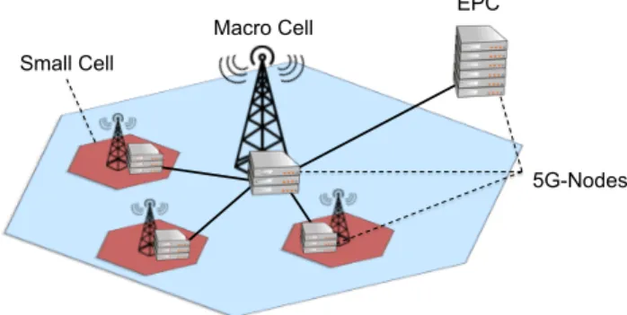
2.3 Optimal Superfluid Management of 5G Networks . . . 27
2.3.1 Architecture Description . . . 28
2.3.2 5G Model . . . 30
2.3.3 Performance Evaluation . . . 34
2.4 Inspired research . . . 37
3 Multicriteria optimization 39 3.1 Multiobjective linear programming . . . 40
3.1.1 Solving MOLP in Objective Space: Bensons’s algorithm . . . 43
3.1.2 Duality . . . 46
3.2 Multiobjective integer linear programming . . . 50
3.2.1 Scalarization techniques . . . 51
3.2.2 Other methods . . . 54
4 A new two-phase strategy for solving bi-objective integer network flow problems 57 4.1 Two-phase method for bi-objective combinatorial optimization problems 57 4.2 A recursive procedure for generating all the feasible solutions of a single objective integer network flow problem . . . 59
4.3 Putting things together . . . 61
5 A new algorithm for the bi-objective integer min cost flow problem 63 5.1 State of the art . . . 63
5.2 The general idea of the algorithm . . . 64
5.3 First phase: the dual variant of Benson’s algorithm . . . 66
5.3.1 Benson’s algorithm strategy . . . 67
5.3.2 Main steps . . . 67
5.4 Second phase: a recursive algorithm for generating all feasible flows . 67 5.4.1 Strategy of the recursive algorithm . . . 68
5.4.2 A special case: degeneracy . . . 72
5.4.3 Illustrative example . . . 73
5.4.4 Adaptation of the recursive procedure to the second phase . . 80
5.5 Preliminary Results . . . 82
6 A new algorithm for the bi-objective minimum spanning tree prob-lem 89 6.1 State of the art . . . 89
6.2 Algorithm description . . . 90
6.3 Finding supported efficient solutions . . . 91
6.3.1 The weighted sum method on the flow formulation . . . 91
6.3.2 Benson’s algorithm on the Kipp-Martin formulation . . . 93
6.4 A recursive algorithm for completing the set of efficient solutions . . 94
6.4.1 Procedure for generating all the spanning trees of a graph . . 95
6.4.2 The recursive procedure adapted to the second phase . . . . 98
6.4.3 Illustrative example . . . 99
xi
Introduction
In many real world applications optimization problems arise where it is required to deal simultaneously with more than one criteria. Several examples of such problems, related to different application fields, can be mentioned. In the manufacturing industry, both maximization of the gain and minimization of the pollution associated to the production process have to be considered simultaneously. Analogously in the transport sector energy efficiency and quality of service have to be guaranteed. The same is true in the health-care system, where quality of service and minimization of the costs represent the main decision criteria. In finance, maximization of the profit and minimization of the risk are the primary goals in portfolio selection. Many other examples could be reported, characterized by two or more objectives that usually, as in those mentioned above, are in conflict with each other. Such conflicting relation between criteria, represents the base for the development of the multi-objective programming. Indeed when more than one conflicting goals have to be optimized it is not possible to use the same concept of "best" solution as for a single objective problem. For such a reason a new concept of optimum has been defined, in order to deal with this class of problems. The first definition of optimum in the context of multi-criteria economic decision making was by Francis Y. Edgeworth. Considering two hypothetical consumer criteria, P and π, he asserted that "It is required to find a point (x, y) such that in whatever direction we take an infinitely small step, P and π do not increase together but that, while one increases, the other decreases" (Edgeworth 1881). Pareto was a contemporary of Edgeworth, and in his most famous theory, "The Pareto Optimum", gave his definition of Pareto optimality: "The optimum allocation of the resources of a society is not attained so long as it is possible to make at least one individual better off in his own estimation while keeping others as well off as before in their own estimation" (Pareto 1906). This new definition of optimality implies the existence of more than one Pareto optimal solution (Pareto frontier), equally efficient, for a multi-objective problem. Such solutions are trade-off solutions for the problem and they are incomparable to each other. From the concept of Pareto optimality new techniques were developed for finding the Pareto frontier. As in the single objective case, the complexity of such methodologies increases when integer or binary decisional variables are considered. Several approaches, exact and heuristics, were designed in order to generate the Pareto frontier for multi-objective combinatorial optimization problems. Although several classes of standard optimization models have been studied in their multi-objective version, there still exists a big gap between the solution techniques and the complexity of the mathematical models that derive from the most recent real world applications.
In this thesis such aspect is highlighted with reference to a specific application field, the telecommunication sector, where several emerging optimization problems are characterized by a multi-objective nature. The study of these problems has been the starting point for an assessment of the state of the art in multi-criteria optimization with particular focus on multi-objective integer linear programming. From the current state of the research, two bi-criteria optimization problems, that have important applications also in the telecommunication industry, have been studied: the bi-objective integer minimum cost flow and the bi-objective minimum spanning tree problems. For both of them a two-phase approach has been designed, able to generate a complete set of efficient solutions. This algorithm, with appro-priate changes according with the specific problem, could be applied on a generic bi-objective network flow problem. The results represent a first attempt in the direction to close the gap between the complex models associated with the most recent real world applications and the methodologies to deal with multi-objective programming.
The thesis is structured in the following way: Chapter 1 reports some preliminary con-cepts on graph and networks and a short overview of the main network flow problems; in Chapter 2 some emerging optimization problems are described, mathematically formalized and solved, underling their multi-objective nature. Chapter 3 presents an overview on multicriteria optimization. Chapter 4 describes the general idea of a new solution algorithm proposed for integer network flow problems. Chapter 5 is focused on the bi-objective integer minimum cost flow problem and on the adaptation of the procedure proposed in Chapter 4 on this problem. Analogously, Chapter 6 describes the application of the same approach on the bi-objective minimum spanning tree problem. For the integer min cost flow problem, the numerical tests performed on a selection of test instances, taken from the literature, permit to verify that the algorithm finds a complete set of efficient solutions. For the minimum spanning tree problem, we solved a numerical example using two alternative methods for the first phase, confirming the practicability of the approach.
1
Chapter 1
Preliminary concepts
In this chapter the main concepts and definitions that will be used in this work are presented. In Section 1.1 several basic definitions and results from graph theory are recalled (taken from [3], [43] and [65]). In section 1.2, an overview of the main network flow problems and their applications is given (taken from [3] and [64]). Lastly Section 1.3 contains a short description of the network simplex method (from [3]).
1.1
Graphs and related definitions
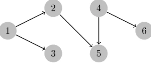
Definition 1 (Directed Graphs). A directed graph G = (N, A) consists of a set
N of nodes and a set A of arcs whose elements are ordered pairs of distinct nodes. A directed network is a directed graph whose nodes and/or arcs have associated numerical values (such as costs, capacities, and/or supplies and demands).
1
2 4
3 5
6
Figure 1.1. Example of directed graph
Definition 2 (Undirected Graphs). An undirected graph G = (N, A) consists of a
set N of nodes and a set A of arcs whose elements are unordered pairs of distinct nodes.
Definition 3 (Tails and Heads). A directed arc (i, j) has two endpoints i and j.
The node i is the tail t(i, j) of arc (i, j) and node j is its head h(i, j). The arc (i, j) is an outgoing arc of node i and an incoming arc of node j.
1
2 4
3 5
6
Figure 1.2. Example of undirected graph
Definition 4 (Degrees). The indegree of a node is the number of incoming arcs of
that node and its outdegree is the number of its outgoing arcs. The degree of a node is the sum of its indegree and outdegree.
Definition 5 (Adjacency List). The arc adjacency list A(i) of a node i is the set
of arcs emanating from that node, that is, A(i) = {(i, j) ∈ A : j ∈ N}. The node adjacency list N(i) is the set of nodes adjacent to that node; in the case of a directed graph, N(i) = {j ∈ N : (i, j) ∈ A}.
Definition 6 (Subgraph). A graph G0 = (N0, A0) is a subgraph of G = (N, A) if
N0 ⊆ N and A0 ⊆ A. Moreover a graph G0 = (N0, A0) is a spanning subgraph of
G = (N, A) if N0 = N and A0 ⊆ A.
Definition 7 (Walk). A walk in a directed graph G = (N, A) is a subgraph of G
consisting of a sequence of nodes and arcs i1− a1− i2− a2− ... − ir−1− ar−1− ir
satisfying the property that for all 1 ≤ k ≤ r − 1, either ak = (ik, ik+1) ∈ A or
ak= (ik+1, ik) ∈ A.
1
2
3 5
Figure 1.3. Example of walk
Definition 8 (Path). A path is a walk without any repetition of nodes.
Definition 9 (Directed Path). A directed path is a directed walk without any
repe-tition of nodes.
Definition 10 (Cycle). A cycle is a path i1− i2 − ... − ir together with the arc
1.1 Graphs and related definitions 3
Definition 11 (Directed Cycle). A directed cycle is a directed path i1− i2− ... − ir
together with the arc (ir, i1).
Definition 12 (Cycle Space). The cycle space of a graph G, denoted by C, is the
smallest set (of undirected arcs or edges) containing the ∅, all cycles in G (where each cycle is treated as a set of edges) and all unions of disjoint cycles in G.
1
2
3
Figure 1.4. Example of cycle
Definition 13 (Acyclic Graph). A graph is acyclic if it contains no directed cycle. Definition 14 (Connectivity). Two nodes i and j are connected if the graph
con-tains at least one path from node i to node j. A graph is connected if every pair of its nodes is connected; otherwise, the graph is disconnected. The maximal connected subgraphs of a disconnected network are its components.
1
2 4
3 5
6
Figure 1.5. Example of connected graph
1
2 4
3 5
6
Figure 1.6. Example of disconnected graph
Proposition 1 (Tree properties).
• A tree on n nodes contains exactly n − 1 arcs.
• A tree has at least two leaf nodes (i.e., nodes with degree 1). • Every two nodes of a tree are connected by a unique path.
Definition 16 (Spanning Tree). A tree T is a spanning tree of G if T is a spanning
subgraph of G.
1
2 4
3 5
6
Figure 1.7. Example of spanning tree for the graph in Figure 1.5
Definition 17 (Fundamental Cycle). Let T be a spanning tree of the graph G. The
addition of any non tree arc to the spanning tree T creates exactly one cycle. Any such cycle is defined a fundamental cycle of G with respect to the tree T .
Definition 18 (Fundamental System of Cycles). Let T be a spanning tree of the
graph G. The fundamental system of cycles of G with respect to T is the set of all fundamental cycles of G with respect to T.
An important result related to the fundamental system of cycles of a graph G with respect to a spanning tree T of G, is Theorem 1. It will be useful in Chapter 5 in order to prove further results.
Theorem 1. Let G be a connected graph and let T be a spanning tree of G. Then
the fundamental system of cycles with respect to G and T forms a basis for the cycle space C.
Proof. Recall first that such a spanning tree T exists when G is connected. Consider
any fundamental cycle C. This cycle is constructed by adding exactly one edge to
T and finding the cycle that results. Thus no fundamental cycle can be expressed
1.2 Network flow problems and main applications 5
least) one edge. As a result, the fundamental system of cycles must be linearly independent.
Choose any element C of C and let {e1, ..., er} be the edges of C that do not appear
in T . Further define the fundamental cycle Ci to be the one that arises as a result of
adding ei to T . The quantity C + C1+ ... + Cr= ∅ if and only if C = C1+ ... + Cr because there are no edges in C that are not in C1+ ... + Cr and similarly no edges
in C1+ ... + Cr that are not in C. It is easy to see that no edge in the set {e1, ..., er}
appears in C + C1+ ... + Cr because each edge appears once in C and once in one of the Ci’s and therefore, it will not appear in C + C1+ ... + Cr. But this means
that every edge in C + C1+ ... + Cr is an edge of T . More specifically, the subgraph
induced by the edges in C + C1+ ... + Cr is a subgraph of T and thus necessarily acyclic. Every element of C induces a subgraph of G that has at least one cycle except for ∅. Thus, C + C1+ ... + Cr= ∅. Since our choice of C was arbitrary we
can see that for any C we have: C = α1C1+ ... + αkCk where {C1, ..., Ck} is the
fundamental set of cycles of G with respect to T and ∀i = 1, ..., k:
αi
(
= 1 if the non-tree edge of Ci is found in C 0 otherwise
Thus, the fundamental set of cycles is linearly independent and spans C and so it is a basis. This completes the proof.
Definition 19 (T -exchange/Cyclic-interchange). Let T be a spanning tree of the
graph G. A T -exchange is a pair of arcs e, f where e ∈ T , f /∈ T , and T − e ∪ f is a spanning tree. The weight of exchange e,f is w(f) − w(e), where w is the vector of the graph weights associated with the arcs.
We recall a combinatorial result related to spanning trees and cyclic-interchanges that will be useful in Chapter 6.
Theorem 2. Let G be a connected graph with n vertices and m edges. Starting
from any spanning tree, one can obtain every other spanning tree of G by cyclic interchanges . Moreover, if T and T0
are two spanning trees, then one can form tree T0 starting from the tree T by at most D(T, T0) cyclic interchanges, where:
D(T, T0) ≤ min{n − 1, m − n + 1}
1.2
Network flow problems and main applications
In this section the main network flow problems are reported together with their most common applications. To this end the concept of flow network and flow on a network are introduced.
Definition 20 (Flow Network). A flow network is a directed graph G = (N, A)
Moreover, to each arc (i, j) ∈ A is assigned a certain upper bound u(i, j) ≥ 0 and lower bound l(i, j) ≥ 0.
Definition 21 (Flow). A flow for a network G = (N, A) is a function f : V ×V → R,
which assigns a real number to each arc (i, j). A flow f is called a feasible flow if it satisfies the following conditions:
(i) l(i, j) ≤ f(i, j) ≤ u(i, j), ∀(i, j) ∈ A.
These are the capacity constraints (if a capacity is ∞, then there is no upper bound on the flow value on that arc).
(ii) For all i ∈ N − {s, t}, the total flow into i is the same as the total flow out of i: X j:(j,i)∈A f (j, i) = X j:(i,j)∈A f (i, j) These are called the flow conservation constraints.
Minimum Cost Flow Problem
The minimum cost flow model is the most fundamental among the network flow problems. This model has several applications: the distribution of a product from manufacturing plants to warehouses, or from warehouses to retailers; the flow of raw material and intermediate goods through the various machining stations in a production line; the routing of automobiles through an urban street network; and the routing of calls through the telephone system.
Mathematical formulation
Let G = (N, A) be a directed network defined by a set N of n nodes and a set A of m directed arcs. Each arc (i, j) ∈ A has an associated cost cij that denotes the
cost per unit flow on that arc. It is assumed that the flow cost varies linearly with the amount of flow. It is also associated with each arc (i, j) ∈ A a capacity uij
that denotes the maximum amount that can flow on the arc and a lower bound lij
that denotes the minimum amount that must flow on the arc. Moreover at each node i ∈ N is associated an integer number b(i) representing its supply/demand. If
b(i) > 0, node i is a supply (or excess) node; if b(i) < 0, node i is a demand (or
deficit) node with a demand of −b(i); and if b(i) = 0, node i is a transshipment node. The decision variables in the minimum cost flow problem are arc flows and are represented by xij ≥ 0 ∀(i, j) ∈ A. The minimum cost flow problem is an
optimization model formulated as follows: min X
(i,j)∈A
cijxij (1.1)
1.2 Network flow problems and main applications 7 X j:(i,j)∈A xij− X j:(j,i)∈A xji= b(i) ∀i ∈ N (1.2) lij ≤ xij ≤ uij ∀(i, j) ∈ A (1.3) where Pn i=1b(i) = 0.
We will refer to the constraint (1.2) as flow conservations constraint. For any node the first term in the above constraint represents the total outflow of the node (i.e., the flow emanating from the node) and the second term represents the total inflow of the node (i.e., the flow entering the node). The flow conservation constraint guarantees that the difference between outflow and inflow is equal the supply/demand of the node. If the node is a supply node, its outflow exceeds its inflow; if the node is a demand node, its inflow exceeds its outflow; and if the node is a transshipment node, its outflow equals its inflow. The flow must also satisfy the lower bound and capacity constraints (1.3). The flow bounds typically model physical capacities or restrictions imposed on the flows operating ranges. In most applications, the lower bounds on arc flows are zero.
Definition 22 (Augmenting cycle). A cycle W (not necessarily directed) in G is
called an augmenting cycle with respect to the flow x if:
i) by augmenting a positive amount of flow around the cycle, the flow remains feasible.
ii) the augmentation increases the flow on forward arcs and decreases the flow on backward arcs in the cycle.
Definition 23 (Incremental/Residual graph). Given a feasible flow x for the min
cost flow problem on the network G = (N, A), the incremental graph is a directed graph Gx= (N, Ax) with arc costs cx and arcs distinguished as follows:
a+∈ A+x ∀a ∈ A : xa< ua
a−∈ A−x ∀a ∈ A : xa> la
Let Ax= A+x ∪ A−x, the arcs in Ax have the following relationship with the arcs in
A: for each a+ ∈ Ax t(a+) = t(a), h(a+) = h(a) and cx
a = ca; for each a− ∈ Ax
t(a−) = h(a), h(a−) = t(a) and ca− = −ca.
Observation 1. W is an augmenting cycle with respect to a feasible flow x if and
only if W corresponds to a directed cycle in the residual network Gx.
Moreover we recall some well-known results that will be useful in Chapter 5 for proving further results.
Theorem 3 (Flow Decomposition Theorem). Every path and cycle flow has a unique
represented as a path and cycle flow with the following two properties:
i) Every directed path with positive flow connects a deficit node with an excess node.
ii) At most n + m paths and cycles have non-zero flow and at most m cycles have non-zero flow. If the flow x is integral, then so are the path and cycle flows which it decomposes.
Proof. The following algorithm finds the set S consisting of at most n + m paths
and cycles with non-zero flow. S = ∅
while there exists a deficit node i
Follow arcs with positive flows starting from i until either an excess node j is found or a node is visited twice.
If an excess node j is found
P is the path from i to j
The flow on the path P is f low(P ) = min{−b(i), b(j), flow of some arc in P } S = S ∪ P
If a node k is visited twice
W is the cycle from k to k
The flow on the cycle W is f low(W ) = min{flow of some arc in W } S = S ∪ W
end while
while there exists an arc a with positive flow
Follow backward arcs with positive flows starting from a until a node is visited twice. Let W be the cycle obtained, then f low(W ) = min{flow of some arc in W } and S = S ∪ W
end while
end procedure
A deficit node exists if and only if an excess node exists, then after the execu-tion of the first while block there are no more imbalanced nodes.
At each iteration either one node becomes balanced or the flow of some arc becomes 0, then there are at most n + m iterations and, as a consequence, n + m paths or
1.2 Network flow problems and main applications 9
cycles.
Whenever a cycle is obtained the flow of some arc becomes 0, then there are at most
m cycles.
Consequence of Theorem 3 is Corollary 1.
Corollary 1. If there are no deficit or excess nodes in the network, then a
non-negative flow x can be represented as at most m cycles with non-zero flow.
Another fundamental result that is consequence of Theorem 3 is the so called Aug-menting Cycle Theorem.
Theorem 4 (Augmenting Cycle Theorem). Let x and x0 be two feasible flows. Then
x equals x0 plus the flow on at most m directed cycles in G(x0). Furthermore the
cost of x equals the cost of x0 plus the cost of the flows on these augmenting cycles.
Proof. For the hypothesis we have:
x = x0+ x0
where x0 is a flow in the residual network G(x0). Since the residual network G(x0) does not have deficit and excess nodes, it follows, from Corollary 1, that x0 can be decomposed in at most m directed flow cycles in G(x0).
Shortest path problem
The shortest path problem is one of the simplest network flow problems. In this problem the goal is to find a directed path of minimum cost (or length) from a specified source node s to another specified sink node t, assuming that each arc (i, j) ∈ A has an associated cost (or length) cij. Some of the simplest applications of the shortest path problem are to determine a path between two specified nodes of a network that has minimum length, or a path that takes least time to traverse, or a path that has the maximum reliability. It can be mathematically formulated as a minimum cost flow problem defining b(s) = 1, b(t) = −1, and b(i) = 0 for all other nodes. This basic model has applications in many different fields, such as equipment replacement, project scheduling, cash flow management, message routing in communication systems, and traffic flow through congested cities.
Maximum flow problem
The maximum flow problem can be seen like a complementary model to the shortest path problem. The shortest path problem models situations in which flow implies a cost but is not restricted by any capacities; in the maximum flow problem flow doesn’t imply costs but is restricted by flow bounds. The maximum flow problem consists in finding a feasible solution that sends the maximum amount of flow from a specified source node s to another specified sink node t. Examples of the maximum flow problem include determining the maximum flow of petroleum products in a pipeline network, cars in a road network, messages in a telecommunication network, and electricity in an electrical network. This problem can be formulated as a mini-mum cost flow problem in the following way. Let b(i) be equal to 0 for all i ∈ N ,
flow bound uts = ∞. Then the minimum cost flow solution maximizes the flow on
arc (t, s); but since any flow on arc (t, s) must travel from node s to node t through the arcs in A, the solution to the minimum cost flow problem will maximize the flow from node s to node t in the original network.
Assignment problem
The data of the assignment problem are represented by two equally sized sets N1 and N2, a collection of pairs A ∈ N1× N2 representing possible assignments, and a cost cij associated with each element (i, j) ∈ A. In the assignment problem the goal
is to pair, at minimum possible cost, each object in N1 with exactly one object in N2.
Examples of the assignment problem include assigning people to projects, jobs to machines, tenants to apartments, and medical school graduates to available intern-ships. Also the assignment problem can be written as a minimum cost flow problem considering the network G = (N1∪ N2, A) with b(i) = 1 ∀i ∈ N1, b(i) = −1 ∀i ∈ N2,
and uij = 1 ∀(i, j) ∈ A.
Transportation problem
The transportation problem is a special case of the minimum cost flow problem with the property that the node set N is partitioned into two subsets N1 and N2 (of
possibly unequal cardinality) so that: (1) each node in N1 is a supply node, (2) each node N2 is a demand node, and (3) for each arc (i, j) ∈ A, i ∈ N1 and j ∈ N2. The
classical example of this problem is the distribution of goods from warehouses to customers. In this context the nodes in N1 represent the warehouses, the nodes in
N2 represent customers (or, more typically, customer zones), and an arc (i, j) ∈ A
represents a distribution channel from warehouse i to customer j. Circulation problem
The circulation problem is a minimum cost flow problem with only transshipment nodes; that is, b(i) = 0 ∀i ∈ N . A feasible flow x must satisfy the lower and upper bounds lij and uij imposed on each arc flow variable xij. Since no exogenous flow is ever introduced to or extracted from the network, all the flow circulates around the network. The goal is to find the circulation that has the minimum cost. The design of a routing schedule of a commercial airline provides one example of a circulation problem. In this setting, any airplane circulates among the airports of various cities; the lower bound lij imposed on an arc (i, j) is 1 if the airline needs to provide service between cities i and j, and so must dispatch an airplane on this arc. Multicommodity flow problems
The minimum cost flow problem models the flow of a single commodity over a network. Multicommodity flow problems arise when several commodities use the same underlying network. The commodities may either be differentiated by their physical characteristics or simply by their origin-destination pairs. Different com-modities can have different origins and destinations, and comcom-modities have separate flow conservation constraints at each node. However, the sharing of the common arc capacities binds the different commodities together. In fact, the essential issue addressed by the multicommodity flow problem is the allocation of the capacity of each arc to the individual commodities in a way that minimizes overall flow costs.
1.2 Network flow problems and main applications 11
Multicommodity flow problems arise in many practical situations, including the transportation of passengers from different origins to different destinations within a city; the routing of nonhomogeneous tankers (in terms of speed, carrying capability, and operating costs); the worldwide shipment of different varieties of grains, from countries that produce grains to those that consume them; and the transmission of messages in a communication network between different origin-destination pairs. Minimum spanning tree problem
A spanning tree is a tree (i.e., a connected acyclic graph) that covers all the nodes of an undirected network G = (V, E) with | V |= n. The cost of a spanning tree is the sum of the costs (or lengths) of its edges. In the minimum spanning tree problem, the goal to identify a spanning tree of minimum cost (or length). The applications of the minimum spanning tree problem are quite diversified and include constructing highways or railroads spanning several cities; laying pipelines connecting offshore drilling sites, refineries, and consumer markets; designing local access networks; and making electric wire connections on a control panel. In its original mathematical formulation it is not written as a min cost flow problem, but as an integer linear programming problem like below.
Mathematical formulation (exponential number of constraints)
min X (i,j)∈E cijxij (1.4) subject to X (i,j)∈E xij = n − 1 (1.5) X (i,j)∈E(S) xij ≤| S | −1 ∀S ⊆ V, S 6= ∅ (1.6) xij ∈ {0, 1} (1.7)
This formulation is the integer linear program for the problem of minimizing the total cost (or length) of a spanning tree for the network under consideration. Constraint (1.5) guarantees that the total number of edges in the spanning tree is equal to
n − 1 as stated in Proposition 1. Constraints (1.6) are called subtour elimination
constraints and ensure that no subgraph induced by S, a generic subset of the network nodes, contains a cycle. Because of these constraints, this formulation is an exponential-sized integer linear program. A possible alternative formulation for the minimum spanning tree problem, with a polynomial number of constraints, can be obtained representing it as a minimum cost flow problem with additional binary variables for each edge, representing if the edge is utilized or not, and an additional constraint which limits the total number of utilized edges to be exactly n − 1 (see [64]). More precisely, a network flow problem is formulated based on the same network in which one node is assumed to be a source sending n − 1 units of flow to all other nodes, each one requiring one unit of flow. It can be easily seen that the solution of this problem is a spanning tree.
Mathematical formulation (polynomial number of constraints)
Considering node 1 as source, the following single commodity flow problem is defined: minX e∈E cexe (1.8) subject to X j:(1,j)∈E f1j − X j:(j,1)∈E fj1 = n − 1 (1.9) X j:(i,j)∈E fji− X j:(j,i)∈E fij = 1, ∀i ∈ V, i 6= 1 (1.10) fij ≤ (n − 1)xe ∀e = (i, j) ∈ E (1.11) fji ≤ (n − 1)xe ∀e = (i, j) ∈ E (1.12) X e∈E xe= n − 1 (1.13) fij, fji≥ 0 ∀e = (i, j) ∈ E (1.14) xe∈ {0, 1} ∀e ∈ E (1.15)
The formulation (6.1) to (6.8) models the minimum spanning tree problem by means of a single commodity flow problem, taking one node as source of n − 1 units of flow, while the other nodes are sinks demanding one unit of flow. Two sets of variables are introduced, the flow variables fij denoting the flow on edge (i, j) (note that although
the arcs are undirected, the flow variables are directed), and the binary variables xe
denoting if the edge e is chosen in solution. Constraints (1.9) and (1.10) model the flow balances at the nodes. Constraints (1.11) and (1.12) force the flow variables associated to edges not in solution to be equal to 0. Constraint (1.13) guarantees that the topology of the solution is a spanning tree. Then, solving this formulation, one can find the minimum spanning tree of the network.
1.3
Network simplex method
The simplex method is widely used for general linear programming programs and has specific implementations for network flow problems. In practice the general simplex method, when implemented without exploiting the underlying network structure, is not a competitive solution procedure for solving the minimum cost flow problem. Fortunately, as these problems have a special structure, it was possible to adapt and interpret the core concepts of the simplex method appropriately as network operations, producing a very efficient algorithm, that is the network simplex algorithm. As explained in [3], when the original network has positive lower bound capacities, it can be transformed into a network with zero lower bound capacities. Therefore, we assume lij = 0 in the following.
The central concept underlying the network simplex algorithm is the notion of spanning tree solutions, that is solutions obtained by fixing the flow of every arc not in the spanning tree either at zero or at the upper bound of the arc and then
1.3 Network simplex method 13
by solving only for the flow on all the arcs in the spanning tree. The procedure consists in moving from one such solution to another, at each step, introducing one new non-tree arc into the spanning tree in place of one tree arc. The name network simplex algorithm derives from the fact that the spanning trees correspond to the so-called basic feasible solutions of linear programming, and the movement from one spanning tree solution to another corresponds to the so-called pivot operation of the general simplex method.
1.3.1 Fundamentals results
As previously mentioned, the network simplex method moves among spanning tree solutions. This is based on the central result of Theorem 5.
Theorem 5 (Spanning Tree Property). The minimum cost flow problem always has
an optimal spanning tree solution.
A spanning tree solution is characterized by a partition of the arc set A in three subsets: T , the arcs in the spanning tree; L, the nontree arcs with flow equal to the lower bound; and U , the nontree arcs with flow equal to the upper bound. The triple (T, L, U ) is called spanning tree structure. At each spanning tree structure it is possible to associate a spanning tree solution, setting xij = 0 ∀(i, j) ∈ L,
xij = uij∀(i, j) ∈ U and then solving the flow conservation constraints to determine
the flow values for the arcs in T . A spanning tree structure is feasible if its associated spanning tree solution satisfies all of the arcs flow bounds. A spanning tree structure is optimal if its associated spanning tree solution is an optimal solution of the minimum cost flow problem. Theorem 6 states a sufficient condition for a spanning tree structure to be optimal.
Theorem 6 (Minimum Cost Flow Optimality Conditions). A spanning tree
struc-ture (T, L, U) is optimal for the minimum cost flow problem if it is feasible and for some choice of node potentials π, the arc reduced costs cπ
ij satisfy the following
conditions: • cπ ij = 0 ∀(i, j) ∈ T • cπ ij ≥ 0 ∀(i, j) ∈ L • cπ ij ≤ 0 ∀(i, j) ∈ U
The reduced cost cπij = cij − π(i) + π(j) for a nontree arc (i, j) ∈ L denotes the
change in the cost of the flow that can be realized by sending 1 unit of flow from node
i to node j through the arc (i, j) appropriately modifying the flow on the arcs in
the tree path between node i and node j. The network simplex algorithm maintains a feasible spanning tree structure and moves from one spanning tree structure to
another until it finds an optimal structure. At each iteration, the algorithm adds one arc to the spanning tree in place of one of its current arcs. The entering arc is a nontree arc violating its optimality condition. Because of its relationship to the primal simplex algorithm for the linear programming problem, this operation of moving from one spanning tree structure to another is known as a pivot operation, and the two spanning trees structures obtained in consecutive iterations are called adjacent spanning tree structures.
1.3.2 Algorithm scheme
The network simplex algorithm maintains a feasible spanning tree structure at each iteration and successively transforms it into an improved spanning tree structure until it becomes optimal. The essential steps of the method are described in the following scheme:
1. Determine an initial feasible tree structure (T, L, U );
Let x be the flow and π be the node potentials associated with this tree structure; 2. while(some nontree arc violates the optimality conditions)
3. select an entering arc (k, l) violating its optimality condition; 4. add arc (k, l) to the tree and determine the leaving arc (p, q); 5. perform a tree update and update the solutions x and π; 6. end while
Each step of this procedure can be implemented in different ways. Moreover, according with the specific network flow problem under consideration, the network simplex method can be specialized in several versions (see [3]).
15
Chapter 2
Emerging optimization
problems in Telecommunication
networks
In this chapter new emerging optimization problems on Telecommunication (TLC) networks are described, mathematically modeled, and solved on a real or realistic scenarios. These results published in [21], [23], [22] and [5] are significative from the point of view of the application, but it will be pointed out that the multiple objective nature of these problems calls for new advances also from the methodological viewpoint for fundamental problems in multi-objective optimization.
2.1
Managing the Energy-Lifetime Trade-off in
Back-bone Networks
This section contains the main results from an operations research perspective of the paper [22] published in Transactions on Networking, 2017. During the last few years, the problem of "green" backbone networks has gained significant importance, starting from the seminal work of Gupta and Sigh [44]. The goal of green networking is to exploit the power management policies to reduce the network energy cost. In particular, a Sleep Mode (SM) is defined: when a SM state is set for a device, the other devices that remain powered on have to sustain the traffic between source and destination nodes. In this context, different works (see for example [1], [42], [24], [17]) have investigated the management of Internet Provider (IP) backbone networks by adopting SM. The main outcome of these works is that networks with SM capabilities are able to save energy, due to the fact that the traffic varies between day and night, resulting in a large number of resources that can be put in SM during the off-peak hours.
However, the impact of SM on the reliability of network devices is an open issue [82], [20]. In particular, there are two opposite effects influencing the lifetime of network devices [20]: the SM duration, which tends to increase the lifetime, and the change in the power state (from SM to full power and viceversa), which instead decreases the lifetime. In general, when a network device experiences a failure, the traffic
flowing on it may be dropped, resulting in a Quality of Service (QoS) degradation for users. Additionally, reparation costs are incurred, which may involve even the replacement of the whole device. In particular, the reparation costs may even exceed the monetary savings derived from SM [81]. All these facts suggest that the device lifetime plays a crucial role in determining the efficiency of SM, and the energy saving may not be the only metric to prove the effectiveness of a SM-based approach. In [19] a simple model to evaluate the lifetime increase/decrease of network devices taking into account the SM duration and its frequency, has been proposed. The model shows that the energy-aware algorithms have an impact on the device lifetime, which may be positive or negative, depending on the Hardware (HW) components used to build the device and on the strategy adopted for choosing which devices should be put in SM. In this context, a natural and interesting problem is related to the possibility of managing SM while always limiting the impact on the lifetime. In this section, to this end, a mathematical formulation of the lifetime-aware problem, over a backbone network, will be described and effectively solved.
2.1.1 Related work
Previous works on green networking are mainly focused on reducing the energy-consumption of devices (see e.g. [13] and [28] for detailed surveys). To this end, different approaches have been proposed, ranging from centralized solutions [42], [24], [17] (i.e., one central controller that decides which elements in the network to put in SM) to distributed solutions [25], [52], [83] (i.e., each node decides which of its own devices to put in SM). All these solutions prove the effectiveness of saving energy by exploiting two main features: i) the fact that current backbone networks are normally over-dimensioned, and ii) the variation of traffic between peak and off-peak hours. However, the impact on the device lifetime is not considered. Traditionally, the node lifetime has been investigated in the context of Wireless Sensors Networks (WSNs) [15], [57], where each node of a WSN is powered by a battery, and therefore it is important to prolong the lifetime of the network, i.e., to avoid the case in which some devices exhaust the battery and then source and destination nodes become disconnected. In general, there are different constraints that may limit the application of power management policies in a network. Usually, guaranteeing protection is one of them [4], [38], [63]. Other constraints include the limitation in the increase of the path length [2], [84], the network delay [61], or the signal quality [16].
In this context, two main reasons suggest to include the lifetime: i) a lifetime decrease may increase the reparation and replacement costs in order to fix the failed devices, and ii) when a device fails, the QoS may be heavily impacted. According with this observation a methodology in order to manage the lifetime while allowing devices to exploit power management primitives is proposed. Such a methodology is based on the idea that the lifetime-awareness should be integrated in the process of deciding when and for how long a power state should be applied to a device.
2.1 Managing the Energy-Lifetime Trade-off in Backbone Networks 17
2.1.2 Modeling the device lifetime
Focusing on the links of an IP backbone network, the generic failure rate for a link at full power is denoted with γon. When SM is applied to the link, the new failure rate γtot is defined as:
γtot = γon(1 −τ s T ) + γ sτs T + ftr NF
where τs is the total time in SM during time period T , γs is the failure rate in SM (which is supposed to be lower than γon), ftr is the power switching rate between full power and SM, and NF is a parameter called number of cycles to failures. The main assumptions behind such a definition are that failures are statistically independent from each other, and their effects are additive. In order to evaluate the lifetime increase/decrease w.r.t. the always on solution (i.e., all links powered on), we define a metric called acceleration factor (AF) (see [20]), which is the ratio between the failure rate with SM γtot and the one at full power γon. The AF metric is lower than 1 if the link lifetime is increased compared to the always on solution. On the contrary, a value larger than 1 means that the lifetime is decreased compared to the always on case. More formally the acceleration factor is defined as follows:
AF = γ tot γon = 1 − (1 − AF s)τs T + χf tr
where AFs is defined as γγons , which is always lower than 1 since the failure rate in
SM γs (by neglecting the negative effect due to power state transitions) is always lower than the failure rate at full power γon. Moreover, χ is defined as 1
γonNF, which
acts as a weight for the power switching rate ftr. The AF is then composed of two terms: the first one which tends to increase the lifetime (i.e., the longer period of SM tends to increase this term which is negative), while the second one instead tends to decrease the lifetime (i.e.,the more often power state transitions occur, the higher this term is). Moreover, the model is composed by parameters AFs and χ, which depend solely on the HW components used to build the link, while parameters τs and ftr depend instead on the realization of SM.
2.1.3 Mathematical Formulation
The goal of the problem under consideration is to minimize the AF in a network exploiting link SM. That is, given the set of nodes and links in the network, and the traffic for each time slot, the objective is the minimization of the average AF over the whole time period, subject to connectivity and maximum link utilization for each time slot. More formally, let G = (V, E) be the network topology. Let V be the set of the network nodes, while E is the set of network links, being | V |= N and | E |= L, respectively. Let us denote with T the total amount of time under consideration. T is divided in K time slots of period δT. Moreover, let ts,d(k) ≥ 0
be the traffic demand from node s to node d during slot k. The problem described above is mathematically modeled as follows:
min 1
L X
(i,j)∈E
The goal is to minimize the average AF of the links in the network. Moreover the traffic has to be routed in the network for each time slot through the following demand satisfaction and flow conservation constraints:
X j:(i,j)∈E fi,js,d(k) − X j:(j,i)∈E fj,is,d(k) = ts,d(k) if i = s −ts,d(k) if i = d 0 if i 6= s, d ∀i, s, d, k (2.2)
where fi,js,d(k) ≥ 0 is the amount of flow from s to d that is routed through link (i, j) during slot k. The total amount of flow fi,j(k) ≥ 0 on each link for each slot is given by:
fi,j(k) =
X
s,d
fi,js,d(k) ∀(i, j) ∈ E, ∀k (2.3) Let ci,j > 0 be the capacity of the link (i, j) and α ∈ (0, 1] be the maximum link
utilization that can be tolerated, respectively. Moreover, the binary variable xi,j(k),
which takes value of 1 if link (i, j) is powered on during slot k, zero otherwise, is introduced. The total amount of flow has to be smaller than ci,j, scaled by the
maximum link utilization α. Such a condition is imposed by the following capacity constraints:
fi,j(k) ≤ αci,jxi,j(k) ∀(i, j) ∈ E, ∀k (2.4)
Note that these constraints impose also the fact that a link has to be powered on if the flow on it is larger than zero. The link state has to be the same in both directions (it is assumed that SM can be set only if the links in both directions are not carrying any traffic):
xi,j(k) = xj,i(k) ∀(i, j) ∈ E, ∀k (2.5)
Then the binary variable zi,j(k), which takes value of 1 if link (i, j) has experienced a power state transition from slot (k − 1) to slot k, zero otherwise, is defined. The value of zi,j(k) is set with the following two constraints:
(
xi,j(k) − xi,j(k − 1) ≤ zi,j(k)
xi,j(k − 1) − xi,j(k) ≤ zi,j(k)
∀(i, j) ∈ E, ∀k (2.6) Then the integer variable Ci,j ≥ 0, which counts the total number of transitions for
each link during the whole time period is introduced:
Ci,j = K
X
k=1
zi,j(k) ∀(i, j) ∈ E (2.7)
Additionally, the variable τi,js ≥ 0, which instead computes the total time in SM for each link, is defined:
τi,js =
K
X
k=1
2.1 Managing the Energy-Lifetime Trade-off in Backbone Networks 19
The variable AFi,j ≥ 0 to compute the total AF for each link is given by:
AFi,j = [1 − (1 − AFi,js )
τi,js
T + χ(i,j) Ci,j
2 ] ∀(i, j) ∈ E (2.9) The variable Ci,j is divided by 2 because a power cycle is always composed by at least two transitions (i.e., from full power to SM, and then from SM to full power). The formulation above includes both integer variables and continuous ones. As a result, it belongs to the class of Mixed Integer Linear Programming (MILP) problems. For this model, a set of inequalities which depend on the specific structure of our problem (following a similar procedure to [9]) has been identified. In this way, the search space was reduced in order to speed up the solution procedure while limiting the amount of time required to generate such inequalities. A more formal description of these inequalities is given below.
Valid inequalities
Let B be the set of source nodes in the network and let δ+(B) be the set of the outgoing edges from B. Then, focusing on the constraints (2.2), (2.3), (2.4) limited to the edges of the set δ+(B):
X s:(s,j)∈E fs,js,d(k) − X j:(j,s)∈E fj,ss,d(k) = ts,d(k) ∀s ∈ B, ∀k, ∀d (2.10) fs,j(k) ≥ X d fs,js,d(k) ∀j : (s, j) ∈ E, ∀s ∈ B, ∀k (2.11) fs,j(k) ≤ αcs,jxs,j(k) ∀j : (s, j) ∈ E, ∀s ∈ B, ∀k (2.12)
Lemma 1. Given Eq. (2.10), (2.11), (2.12) the following valid inequalities hold:
X (i,j)∈δ+(B) ci,jxi,j(k) ≥ 1 α X s∈B,d ts,d(k) ∀k (2.13)
Proof. From constraint (2.10) we can write: X
s:(s,j)∈E
fs,js,d(k) ≥ ts,d(k) ∀s ∈ B, ∀k, ∀d (2.14) If we consider the sum on all destinations we obtain:
X d X s:(s,j)∈E fs,js,d(k) ≥X d ts,d(k) ∀s ∈ B, ∀k (2.15) From constraints (2.11) and (2.12) it is also possible to write:
X d X s:(s,j)∈E fs,js,d(k) = X s:(s,j)∈E X d fs,js,d(k) ≤ X s:(s,j)∈E fs,j(k) ≤ α X j:(s,l)∈E cs,jxs,j(k) ∀s ∈ B, ∀k (2.16)
Additionally, from constraints (2.15) and (2.16) we obtain: α X j:(s,l)∈E cs,jxs,j(k) ≥ X s∈B,d ts,d(k)∀s ∈ B, ∀k (2.17) or equivalently: X j:(s,l)∈E cs,jxs,j(k) ≥ 1 α X d ts,d(k)∀s ∈ B, ∀k (2.18) If we consider the sum on all sources we can write:
X s∈B X j:(s,l)∈E cs,jxs,j(k) ≥ 1 α X s∈B,d ts,d(k) ∀k (2.19) that is: X (i,j)∈δ+(B) ci,jxi,j(k) ≥ 1 α X s∈B,d ts,d(k) ∀k (2.20)
The formulation obtained adding the set of valid inequalities (2.13), as shown by the experimental results in the next section, is an enhanced formulation that speeds up the solution procedure.
2.1.4 Experimental Results
The reference scenario has been provided by Orange-FT (see [54]). The operator has provided the topology in terms of nodes and links, link capacities, routing weights, and the traffic variation over one working day, with a time granularity of one hour between one traffic matrix and the following one (see [53] for a detailed description of this scenario). Moreover, the maximum link utilization is set to 50% of the link capacity, as suggested by the operator.
A time period T equal to four days has been considered. Unless otherwise specified, six different traffic matrices equally spaced for each day have been used (always including the peak traffic matrix in the matrix set). Moreover, these matrices were repeated over the different days. This is a conservative assumption, since the traffic during weekends may be lower compared to working days, but the obtained results are representative. Moreover the same HW parameters for the links were assumed, i.e., all links are deployed with similar devices in terms of HW characteristics. The original formulation has been solved with CPLEX solver (version 12.6) on a high performance computing cluster, composed of four nodes, each of them with 32 cores and 64 GB of RAM, for a total computing power of around 1.5 TeraFlops/s. The average AF, the time required to retrieve the solution, and the optimality gap were considered as performance metrics. Table 2.1 reports the obtained results (the optimality gap is expressed in percentage), for different HW parameters AFi,js and χi,j. Recall that AFi,js is the AF of the device when a SM state is applied (without considering transitions), while χi,j is the weight for the frequency of power
2.1 Managing the Energy-Lifetime Trade-off in Backbone Networks 21
Figure 2.1. Orange-FT network topology
yet available in the literature, a sensitivity analysis w.r.t. both of them has been preformed. Moreover, a maximum time limit of 24h for retrieving the solution from the optimization solver has been imposed.
Table 2.1. Optimization Results
AF(i,j)sleep χi,j Objective Gap(%) Time
0.2 0.01 0.71 4.18 24h 0.2 0.05 0.79 2.68 24h 0.2 0.1 0.87 2.4 24h 0.2 0.5 0.94 0 46’ 32” 0.2 1 0.94 0 41’ 18” 0.5 0.01 0.83 1.98 24h 0.5 0.05 0.90 2.21 24h 0.5 0.1 0.96 0.21 24h 0.5 0.5 0.97 0 44’ 32” 0.5 1 0.97 0 22’ 33” 0.8 0.01 0.94 0.65 24h 0.8 0.05 0.99 0 1h 10’ 0.8 0.1 0.99 0 1h 36’ 0.8 0.5 0.99 0 53’ 0.8 1 0.99 0 51’ 20”
In eight out of the fifteen runs we found the optimal solution, in the other cases we have a gap less or equal to 4.18%.
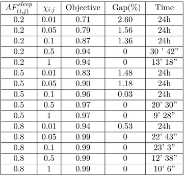
In Table 2.2 the optimization results of the improved model are shown. As we can see, the convergence to the optimum is faster with respect to the original model. In the other cases the gap between the objective function and the lower bound found within the time limit, is lower.
Table 2.2. Optimization Results (with valid inequalities)
AF(i,j)sleep χi,j Objective Gap(%) Time
0.2 0.01 0.71 2.60 24h 0.2 0.05 0.79 1.56 24h 0.2 0.1 0.87 1.36 24h 0.2 0.5 0.94 0 30 ’ 42” 0.2 1 0.94 0 13’ 18” 0.5 0.01 0.83 1.48 24h 0.5 0.05 0.90 1.18 24h 0.5 0.1 0.96 0.03 24h 0.5 0.5 0.97 0 20’ 30” 0.5 1 0.97 0 9’ 28” 0.8 0.01 0.94 0.53 24h 0.8 0.05 0.99 0 22’ 43” 0.8 0.1 0.99 0 23’ 3” 0.8 0.5 0.99 0 12’ 38” 0.8 1 0.99 0 10’ 6”
For low values of AFi,js and χi,j, the problem is very challenging to be solved
optimally: this is due to the fact that the gain in putting devices in SM is high, while at the same time the penalty for introducing transitions is low. Thus, the only constraint limiting the AF decrease is the traffic, which imposes to put at full power different links during peak hours. However, traffic varies during the day, therefore the set of links in SM is varied too. As a consequence, the solver always tries to maximize the number of links in SM, resulting in a low average AF and a high time required to obtain the solution. However, we can see that in all cases, the maximum gap is always below 2.60%. Moreover, when χi,j is increased, the penalty associated to the
power state changes becomes not negligible. This has an impact on the objective function (resulting in a higher AF), but also on lower computation time, due to the fact that the set of links in SM changes less frequently with time. Additionally, when
AFi,js is increased, we can clearly see that the AF tends to increase, since the gain for putting the devices in SM is lower. However, the AF is always lower than one, meaning that the lifetime has been increased compared to the solution in which all links are always powered on. For example, when AFi,js = 0.2 and χi,j = 0.01 [1/h],
the AF is equal to 0.71, resulting in a lifetime increase of almost 30%.
These results show that both the HW and sleep mode parameters play a crucial role for influencing the lifetime. Moreover, they show that the lifetime of a network can be effectively managed applying SM policies.
2.2
Optimal Sustainable Management of Backbone
Net-works
This section contains the main results from an operation research perspective of the paper [5] published in IEEE, International Conference on Optical Networks, 2016.
2.2 Optimal Sustainable Management of Backbone Networks 23
As previously mentioned, even though the reduction of costs in terms of energy brought by sleep mode approaches has been already recognized and accepted by the research community, little efforts have been performed so far to understanding what are the implications of adopting this type of solution in an operator network. In particular, the transition between sleep mode and full power, applied regularly to the devices in a network, may dramatically reduce their lifetime [20]. When the devices decrease their lifetime, they need to be fixed more frequently, thus increasing the associated reparation/replacement costs [82]. As a result, there is a trade-off between the amount of energy that can be saved in a network and the maximum admissible lifetime degradation [21]. Additionally, another effect that has to be considered when adopting energy-efficient solutions is the impact on the Quality of Service (QoS) to users. More in depth, if users are served by few network devices, their experienced QoS may be low compared to the case in which all devices are always powered on. A user experiencing a low QoS may then decide to migrate to another operator, thus again representing a loss for its original operator. In this context, a natural problem that arises is the possibility to trade between network energy savings, device fixing costs, and user QoS in a backbone network. To this end a mathematical formulation in which the total sustainability of a backbone network is maximized, is here proposed. In order to reflect all the aspect above mentioned the total sustainability is expressed as a metric encompassing electricity costs, lifetime costs, and users QoS, as shown in the next section.
2.2.1 Problem Formulation
A backbone network composed of source/destination nodes and purely transport nodes was considered. It was also assumed that the links capacity and the traffic demand by all source/destination node pairs for each time period are given. The objective is to maximize the total sustainability of the network, by jointly considering the users utility, the device fixing costs, and the network energy costs. More in depth, the users utility is defined as a revenue for the operator to serve users at a given rate. The higher is the rate for serving users, the higher is also their utility. In this way, also the QoS for serving the users has been taken into account. By assuming that time is divided in time slots of fixed duration,the target is the maximization of the sustainability in each time slot by acting on the power state of each link in the topology. Each link can be at full power or in sleep mode (SM). More formally, let
G = (V, E) be the graph representing the network infrastructure. Let V be the set
of the network nodes, while E the set of the network links. We assume | V |= N and | E |= L. Let ci,j > 0 be the capacity of the link (i, j) and α ∈ (0, 1] the maximum
link utilization that can be tolerated. It is assumed that the total period of time under consideration is divided in time slots of duration δt. Let k be the current time slot index. The mathematical formulation is then introduced by means of different set of variables. Focusing on traffic, it is assumed a variable amount of traffic for each source s and each destination d. Let tsdmin(k) be the minimum amount of traffic for node pair s − d at time slot k. Similarly, let tsd
max(k) be the maximum amount
of traffic between s and d at time slot k. The continuous variables λsd(k) denote the actual amount of traffic assigned to pair s − d at k. Additionally, fi,js,d(k) ≥ 0 is the amount of flow from s to d that is routed through link (i, j) during current time
slot k. Similarly, fi,j(k) ≥ 0 is the total amount of flow on link (i, j) during slot k.
Given the previous definitions, the problem is formulated as:
max[Utot(k) − (CE(k) + CR(k))] (2.21) The goal is to maximize the total sustainability of the system at each time slot k. The objective function is then given by the difference between the total utility and the total cost at time slot k. This latter is represented by the sum of the total energy cost and the total fixing cost at time slot k.
X j:(i,j)∈E fi,js,d(k) − X j:(j,i)∈E fj,is,d(k) = λs,d(k) if i = s −λs,d(k) if i = d 0 if i 6= s, d ∀i ∈ V (2.22)
The flow conservation constraints guarantee that the traffic is correctly routed in the network. Moreover the following constraints are imposed on the variable λsd(k):
λsd(k) ≤ tsdmax(k) ∀s, d (2.23)
λsd(k) ≥ tsdmin(k) ∀s, d (2.24) The total amount of flow on each link is then given by:
fi,j(k) =
X
s,d
fi,js,d(k) ∀(i, j) ∈ E (2.25) The total amount of flow is limited to be smaller than the link capacity:
fi,j(k) ≤ αci,jxi,j(k) ∀(i, j) ∈ E (2.26)
where xi,j(k) is a binary variable which takes value one if the link (i, j) is powered
on during slot k, zero otherwise.
Considering the users utility, let Umin and Umax be a minimum and a maximum utility value, respectively. Moreover, let λsdmin and λsdmax be the minimum and maxi-mum thresholds for λsd(k). The resulting utility variable Us,d for users requesting traffic from node s to node d is then computed as:
Us,d= Umin if λsd(k) ≤ λsdmin
Umin+ (Umax− Umin) log2(1 +
λsd(k)−λsd min λsd max−λsdmin ) if λsdmin ≤ λsd(k) ≤ λsd max Umax if λsd(k) ≥ λsdmax (2.27) The previous expression assumes that the user utility scales logarithmically with the actual amount of served traffic λsd(k). In this way, the increment of users utility