https://doi.org/10.1140/epjc/s10052-018-6063-y Regular Article - Experimental Physics
Intrinsic mirror noise in Fabry–Perot based polarimeters: the case
for the measurement of vacuum magnetic birefringence
G. Zavattini1,a, F. Della Valle2, A. Ejlli1, W.-T. Ni3, U. Gastaldi1, E. Milotti4, R. Pengo5, G. Ruoso5
1Sez. di Ferrara and Dip. di Fisica e Scienze della Terra, INFN, Università di Ferrara, via G. Saragat 1, Edificio C, 44122 Ferrara, FE, Italy 2Sez. di Pisa, gruppo collegato di Siena and Dip. di Scienze Fisiche, della Terra e dell’Ambiente, INFN, Università di Siena, via Roma 56, 53100
Siena, SI, Italy
3Department of Physics, National Tsing Hua University, Hsinchu 30013, Taiwan, Republic of China 4Sez. di Trieste and Dip. di Fisica, INFN, Università di Trieste, via A. Valerio 2, 34127 Trieste, TS, Italy 5Lab. Naz. di Legnaro, INFN, viale dell’Università 2, 35020 Legnaro, PD, Italy
Received: 10 May 2018 / Accepted: 11 July 2018 © The Author(s) 2018
Abstract Although experimental efforts have been active for about 30 years, a direct laboratory observation of vac-uum magnetic birefringence, due to vacvac-uum fluctuations, still needs confirmation: the predicted birefringence of vacuum is !n= 4.0 × 10⁻²⁴@ 1 T. Key ingredients of a polarimeter
for detecting such a small birefringence are a long optical path within the magnetic field and a time dependent effect. To lengthen the optical path a Fabry–Perot is generally used with a finesse ranging from F ≈ 104to F ≈ 7 × 10⁵.
Interestingly, there is a difficulty in reaching the predicted shot noise limit of such polarimeters. We have measured the ellipticity and rotation noises along with Cotton-Mouton and Faraday effects as a function of the finesse of the cavity of the PVLAS polarimeter. The observations are consistent with the idea that the cavity mirrors generate a birefringence-dominated noise whose ellipticity is amplified by the cav-ity itself. The optical path difference sensitivcav-ity at 10 Hz is S!D= 6 × 10⁻¹⁹m/√Hz, a value which we believe is
con-sistent with an intrinsic thermal noise in the mirror coatings. Our findings prove that the continuous efforts to increase the finesse of the cavity to improve the sensitivity has reached a limit.
1 Introduction
The development of extremely sensitive polarimeters has been driven in recent years by attempts to measure directly vacuum magnetic birefringence, a non linear quantum elec-trodynamic effect in vacuum closely related to light-by-light elastic scattering. Non linear electrodynamic effects in
vac-ae-mail:guido.zavattini@unife.it
uum were first predicted in 1935 by the Euler–Kockel per-turbative effective Lagrangian density [1–12],
LEK = 1 2µ0 !E2 c2 − B2 " +µAe 0 #!E2 c2 − B2 "2 + 7! Ec ·B "2$ , (1)
which takes into account vacuum fluctuations with the cre-ation of electron-positron pairs. As of today, LEK still
needs direct experimental confirmation at low energies. This Lagrangian density is valid for field intensities much lower than the critical values: B ≪ Bcrit = m2ec2/e¯h = 4.4 ×
109T, E≪ E
crit= m2ec3/e¯h = 1.3 × 10¹⁸V/m. Here
Ae= 45µ2 0 α2¯λ3e mec2 = α 90π 1 Bcrit2 = 1.32 × 10 −24T−2, (2)
describes the entity of the quantum correction to Classical Electrodynamics. The Lagrangian density (1) predicts that vacuum becomes birefringent in the presence of either an external electric or magnetic field [8–12]. In the case of an external magnetic field the unitary birefringence, to order α2,
is expected to be, !n B2 = 3Ae= 2 15µ0 α2¯λ3e mec2 = 3.96 × 10 −24T−2. (3)
In the presence of an external electric field, B2is replaced
by− (E/c)2.
Due to this birefringence, a linearly polarised beam of light propagating perpendicularly to the external magnetic field acquires an ellipticity ψ,
ψ = ψ0sin 2ϑ = π %L 0 !n dl λ sin 2ϑ = π3Ae %L 0 B2dl λ sin 2ϑ, (4)
where ψ0 is the ellipticity amplitude, λ is the wavelength
of the light, L is the length of the magnetic field and ϑ is the angle between the magnetic field and the polarisation direction. With the parameters of the PVLAS experiment [13], B= 2.5 T, L = 1.64 m and λ = 1064 nm, the induced ellipticity is ψ= 1.2 × 10⁻¹⁷, an extremely small value. As
we will see in the following section, one way to enhance the induced ellipticity is to increase the effective length of the magnetic field region using a Fabry–Perot cavity with finesse F . Such a cavity enhances an ellipticity (or a rotation) by a factor N = 2F /π [14–17] which, today, can be as high as N= 4.5 × 10⁵[18].
Several experiments are underway, of which the most sen-sitive at present are based on polarimeters with such very high finesse Fabry–Perot cavities [19–22]. Furthermore all of these experiments use variable magnetic fields in order to induce a time dependent effect hence further increasing their sensitivities. This time dependence can be obtained either by varying the magnetic field intensity, in which case !n= !n(t), or by rotating the field direction in a plane per-pendicular to the propagation direction such that ϑ = ϑ(t). In this second case, adopted by the PVLAS experiment [19] with N = 4.5 × 10⁵, the signal to be measured is,
'(t)= Nψ(t) = Nπ3Ae %L
0 B2dl
λ sin 2ϑ(t)
= 5 × 10⁻¹¹sin 2ϑ(t). (5)
At present the lowest measured value for !n/B2is [23],
!nPVLAS/B2= (1.9 ± 2.7) × 10−23T−2. (6) The experimental uncertainty on this value is a factor of about seven above the predicted QED value in Eq. (3).
2 Polarimetry: state of the art
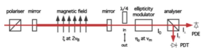
A scheme of the PVLAS polarimeter is shown in Fig.1. A beam first passes through a polariser and then enters the Fabry–Perot cavity composed of two high-reflectance mir-rors placed at a distance D = 3.303 m apart. Between the mirrors is a magnetic field of length L which, in the case of the PVLAS experiment, is generated by two iden-tical rotating permanent magnets characterised by the total parameter%0LB2dl = 10.25 T2m resulting in an average
field B = 2.5 T over a length L = 1.64 m. These two magnets have been rotated up to a frequency νB = 23 Hz.
Given the dependence of the induced ellipticity ψ(t) with
Fig. 1 A polarimeter based on a Fabry–Perot cavity with a
time-dependent signal and heterodyne detection. PDE extinction photodiode;
PDTtransmission Photodiode
2ϑ(t), the ellipticity signal due to magnetic birefringence has a frequency component at 2νB. Since the magnetic field
could in principle also generate rotations φ(t) due to a mag-netic dichroism (for example from axion-like particles [24]) in Fig.1the total effect is indicated with a complex number ξ = φ + iψ. Indeed one can assign an absolute phase to the electric field of the light such that a rotation is described by a pure real number whereas an ellipticity is a pure imag-inary quantity. After the output mirror, an ellipticity modu-lator adds a known ellipticity of amplitude η0 ≪ 1 to the
polarisation at a frequency νm ≫ νB. The beam of power
I0then passes through an analyser (a polariser set to
extinc-tion) which divides the light into two polarisation compo-nents: parallel and perpendicular to the input polariser, I∥ and I⊥ respectively. These beams are collected by the two photodiodes PDT and PDE with efficiencies q= 0.7 A/W. If all ellipticities (and rotations) are small these add alge-braically. In the presence of both a rotation ,(t)= Nφ(t) and an ellipticity '(t)= Nψ(t) (,, ' ≪ 1) and without the presence of the quarter-wave plate shown in Fig.1, the power reaching PDE is
I⊥ell(t)= & beam ϵ0c|E⊥(t)|2d.≃ I0|iη(t)+i'(t) + ,(t)|2 = I0 ' η2(t)+ 2η(t)'(t) + ,(t)2+ '(t)2(. (7) As can be seen, only the ellipticity '(t) beats with the effect of the modulator η(t). The modulation amplitude η0 must
be chosen such that the term η2
0/2 is well above the noise
in the PDE signal: generally ,(t), '(t)≪ η0. If η(t) and
'(t)are sinusoidal functions at frequencies νmand ν
respec-tively (having chosen νm≈ 50 kHz), the product 2η(t)'(t)
generates Fourier components at νm± ν.
By demodulating the current signal from PDE iell ⊥ (t) =
q Iell
⊥ (t)at the frequencies νm and 2νm, one obtains the
in-phase Fourier components,
iνm(ν)= 2I0qη0'0(ν) and i2νm(dc)= q I0η20/2 (8)
from which one can extract the amplitude (with relative sign) for '0: '0(ν)= iνm(ν) 2q I0η0 = iνm(ν) 2)2q I∥i2νm(dc) = η40 iνm(ν) i2νm(dc) . (9)
By inserting the quarter-wave plate with one of its axes aligned with the polarisation, the ellipticity generated by the magnetic field becomes a rotation and vice-versa [25]. In this case, the power reaching PDE is,
I⊥rot(t)= & beam ϵ0c|E⊥(t)|2d.≃ I0|iη(t) ± '(t) ∓ i,(t)|2 = I0 ' η2(t)± 2η(t),(t) + ,(t)2+ '(t)2 ( (10) where the signs depend on whether the polarisation is aligned with the fast or the slow axis of the λ/4 wave plate. Again the value of ,0(ν)can be extracted using the same expres-sions in Eq. (9). We explicitly note that Eqs. (7), (9) and (10) hold for both an ellipticity/rotation signal and for an elliptic-ity/rotation noise.
In the spectra obtained from Eq. (9), an ellipticity gen-erated by a magnetic birefringence or a rotation gengen-erated by a magnetic dichroism will appear at ν = 2νBwhereas a
rotation due to a time dependent Faraday effect at νF will
appear at ν= νF.
Given the scheme in Fig.1, one can determine the expected peak ellipticity sensitivity S'(ν) of the polarimeter in the
presence of various noise sources (see Fig.2). All noise con-tributions will be expressed as electric currents. In general the rms noise measured at the output of the demodulator at a frequency ν is the incoherent sum of the rms noise densities S+and S−respectively at the frequencies νm+ν and νm−ν.
Generally|S+| = |S−| = Sν. Using Eq. (9) one finds,
S'(ν)= √ 2* S2 ++ S−2 2q I0η0 = Sν q I0η0. (11)
The ultimate peak sensitivity S' of such a polarimeter is
given by the shot-noise limit. The rms current spectral density ishotat PDE due to an incident d.c. light power I
⊥(dc) is,
ishot =)2eq I⊥(dc), (12)
constant over the whole spectrum. Equation (11) then leads to, S'shot(ν)= + 2e q I∥ , η20/2+ σ2 -η20 , (13)
where we have introduced the extinction ratio of the polaris-ers σ2and we have introduced I
∥ as a measurement of I0.
If the modulation term is η2
0/2≫ σ2, the above expression
simplifies to, S'shot(ν)=. e q I∥. (14) Iout = 0.7 mW RIN(50 kHz) = 3·10-7 1/√Hz σ2 = 1·10-7 G = 0.7·106 V/W
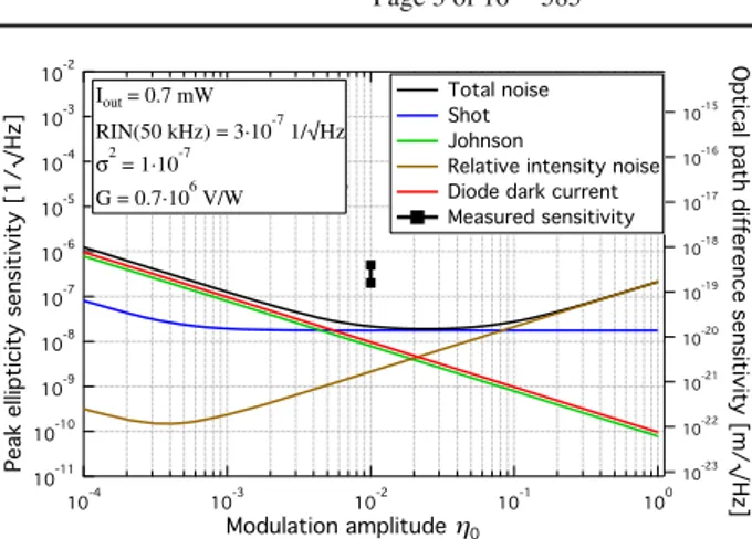
Fig. 2 Noise budget of the principal noise sources as a function of
the modulation amplitude η0for the PVLAS polarimeter. A minimum
which coincides with shot-noise sensitivity exists. Superimposed on the plot is the experimental sensitivity between 10 and 20 Hz with η0= 10−2
Typical working values for the extinction ratio σ2and the
modulation amplitude η0are σ2! 10−7and η0≈ 10−2. The
extinction ratio reported is with the cavity and the modulator crystal inserted. It does not change significantly when the QWP is also inserted. As will be discussed below, the value of the power I0 ≈ I∥ at the output of the cavity used in
the PVLAS setup during the measurements presented in this work is I∥ = 0.7 mW from which one obtains a shot noise peak sensitivity of,
Sshot' (ν)= 1.8 × 10⁻⁸/√Hz. (15) With the effect to be measured '= 5.4×10⁻¹¹and with the
above shot noise the measurement time for a unitary signal-to-noise ratio should be T =,Sshot
' /'
-2
= 1.1 × 10⁵s, in
principle a reasonable integration time.
Considering other known noise sources such as the John-son noise, iJN, the diode dark current noise iDNand the laser’s relative intensity noise iRIN one obtains the curves shown in Fig.2for the sensitivity as a function of the modulation amplitude η0 [19]. As can be seen there is a region in the
modulation amplitude around η0≈ 2 × 10⁻²which should
in principle allow shot noise sensitivity.
The out-of-phase quadrature signal iνqum(ν)at the output of the demodulator can be used as a good measurement of noise contributions uncorrelated to ellipticity noise. In principle, if S'(ν)was limited by one of the wide band noises reported in
Fig.2then iνm(ν)= i
qu
νm(ν). Unfortunately this is not the case and the measured sensitivity of the PVLAS polarimeter when measuring ellipticities with N = 4.5 × 10⁵is significantly
worse than the values in Fig.2: SPVLAS
' ∼ 3−5×10⁻⁷/
√ Hz for frequencies ν∼ 10–20 Hz and η0= 10−2.
To better understand the actual sensitivity reached by the PVLAS experiment one should consider, rather than the
S∆
λ
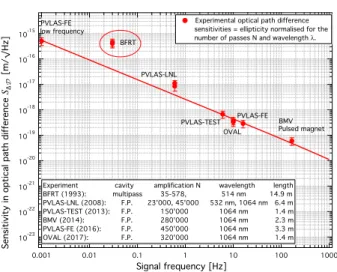
Fig. 3 Measured optical path difference sensitivity for past and present
experiments as a function of their typical working frequency. BFRT [28], PVLAS-LNL [25,29], PVLAS-TEST [30], BMV [21], PVLAS-FE [19], OVAL [22]. The line is a fit with a power law having excluded the BFRT values. The resulting power is (−0.78 ± 0.03)
ellipticity, the sensitivity in optical path difference !D = %
path!n dl:
S!D= S'PVLAS λ
πN ∼ 3− 6 × 10
−19m/√Hz, (16)
between 10 and 20 Hz. This value can be compared to the ones for gravitational wave detection using interferometer techniques [26]. Indeed the quantities to be compared are, S'PVLAS λ
2π N ⇐⇒ hsenslarm, (17)
where larmis the arm length of the gravitational wave
inter-ferometer and hsens is its sensitivity in strain [26]. For
example in Advanced LIGO (Figure 2 of Ref. [27]) with larm= 4000 m and hsens≈ 1.5 × 10⁻²²/√Hz @20 Hz, one finds S!D ≈ 10−18m/√Hz, a value slightly above the one of the PVLAS experiment. It must also be noted that grav-itational wave interferometers are not shot noise limited at these frequencies but are limited by technical noises [27].
Interestingly, all of the past and present experimental efforts also have been limited by a yet to be understood wide band noise. In Fig.3we report the optical path difference sensitivities of past and present experiments dedicated to measuring vacuum magnetic birefringence with optical tech-niques. These sensitivities are plotted as a function of the fre-quencies at which each experiment typically works/worked at. Although each experiment is characterised by a different finesse of the cavity and uses different detection schemes (heterodyne, homodyne), the sensitivities lie on a common power law∝ νx with x = −0.78 ± 0.03. The only
experi-ment significantly above this common curve is BFRT [28].
This is the oldest effort and used a multi-pass cavity with sep-arate optical benches rather than a Fabry–Perot. The mirrors were also of different fabrication. Furthermore all of these sensitivities are well above their expected shot noise limit with the exception of the OVAL experiment which uses a very low power of 10 µW at the output of the cavity and whose sensitivity coincides with its expected one [22].
Finally, without the presence of the Fabry–Perot cavity the PVLAS polarimeter reaches shot-noise sensitivity above ν∼ 10 Hz. Below this frequency the noise is due to point-ing fluctuations of the laser beam coupled to birefrpoint-ingence gradients present in all optical elements.
A possibile interpretation of the general behaviour shown in Fig.3is that there is an intrinsic birefringence noise being generated in the mirror reflective coatings. Given the order of magnitude of the sensitivities in Fig.3we believe that we have reached a thermal intrinsic noise in birefringence, not induced by the laser power, but due to the mirrors in thermal equilibrium at T ≈ 300 K.
To verify whether the excess noise present in the PVLAS experiment is indeed a birefringence noise originating from the reflective coatings of the mirrors we performed a series of measurements both in ellipticity and in rotation as a function of the finesse of our cavity. The measurements were per-formed with a pure birefringence signal due to Argon gas at a pressure P≈ 0.85 mbar and with an external solenoid gen-erating a Faraday rotation on the input mirror of the cavity. In this paper the results of these measurements are presented showing that indeed the excess noise is dominated by bire-fringence noise and that the ellipticity noise is proportional to the finesse of the cavity.
3 Method
The basic scheme of our polarimeter was described above but to fully understand the measurements we are going to present, we must here include some extra details.
3.1 Mirror birefringence
The most important point is that the mirrors of Fabry–Perot cavities always present an intrinsic structured birefringence [32] over the reflecting surface. The composition of the fringence of the two mirrors can be treated as a single bire-fringent element [33] inside a perfect non birefringent cav-ity. If α1and α2are the phase retardations upon reflection
on each mirror for two polarisations parallel and perpendic-ular to their slow axis and if we take as a reference angle the slow axis of the first mirror then, per round trip, the two mirrors are equivalent to a single birefringent element with a total retardation αEQat an angle ϑEQwith respect to the first
αEQ= ) (α1− α2)2+ 4α1α2cos2ϑWP, (18) cos 2ϑEQ= ) α1+ α2cos 2ϑWP (α1− α2)2+ 4α1α2cos2ϑWP , (19)
where ϑWPis the angular position of the slow axis of the
sec-ond mirror. Typical values for α1,2are∼ 10−7to 10−5rad.
This leads to a high finesse cavity having two non degenerate resonances slightly separated in frequency by,
!νsep= νf srαEQ
2π (20)
where νf sr = 2Dc is the cavity’s free spectral range. This
separation is to be compared with each resonance’s FWHM !νcav= νf sr/F .
To reach a good extinction, necessary to have a good sen-sitivity, the input polarisation must be aligned to one of the axes of the cavity’s equivalent birefringence. In this way no component perpendicular to E∥will be generated by the cav-ity itself. The reflected light used to lock the laser to the cavcav-ity has a polarisation parallel to the input polariser. For this rea-son the laser is locked to only one of the two rerea-sonances whereas the ellipticity (or rotation) signal will respond to the resonance shifted by !νsep.
As discussed in Refs. [17,19] the ratio !νsep/!νcav =
Fα2πEQ = 12N α2EQ leads to an extra phase between the two perpendicular polarisation states and to a reduction of the signal. Assuming the presence of only an ellipticity '0the
resulting expression for E⊥(t)is: E⊥(t)= E0 / i'0k(αEQ) ! 1− iN αEQ 2 " sin 2ϑ(t)+ iη(t) 0 (21) where, k(αEQ)= 1 1+ N2sin2(α EQ/2). (22)
The expression for E⊥(t)is actually only valid in the limit of low frequencies with ν≪ !νcav, as will be discussed in
Sect.3.2. Apart from a reduction of the accumulated ellip-ticity '0by a factor k(αEQ), E⊥(t)is no longer a pure
imag-inary number but also has a real component corresponding to a rotation N αEQ
2 k(αEQ)'0. The result of this modification
of E⊥(t)is therefore a mixing of an ellipticity and a rotation by a factorN αEQ
2 . The same mixing occurs in the presence of
a pure rotation.
In the presence of both an accumulated rotation ,0 =
N φ0and an accumulated ellipticity '0 = Nψ0 the
mea-sured ellipticity 'meas
ν→0and the measured rotation ,measν→0can
therefore be determined from (ν≪ !νcav),
'ν→0meas= k(αEQ) / '0− N αEQ 2 ,0 0 , (23) ,measν→0= k(αEQ) / ,0+ N αEQ 2 '0 0 . (24)
Measuring αEQis thus fundamental to disentangle
elliptici-ties and rotations.
Having measured the finesse of the cavity and considering the presence of a pure ellipticity only (,0= 0) one finds that
(ν≪ !νcav), ,measν→0 'νmeas→0 1 1 1 1 ,0=0 = N α2EQ, (25)
gives a direct value for αEQ. The same is true in the presence
of a pure rotation ('0= 0) in which case,
'νmeas→0 ,measν→0 1 1 1 1 '0=0 = −N α2EQ. (26)
The determination of αEQcan therefore be easily done either
by measuring a Cotton-Mouton signal or a Faraday effect, in either case with and without the quarter-wave plate inserted. In the next sections we will see how these must be modified to determine αEQalso for frequencies ν" νcut.
As we will see below, the mixing of an ellipticity with a rotation will also help us understand the origin of the excess noise typically observed in polarimeters based on high finesse cavities.
3.2 Frequency response
In the previous paragraph we introduced the mixing between ellipticities and rotations due to the cavity birefringence in the low frequency limit. Due to the relatively narrow cavity width !νcav ∼ 65 Hz with respect to the frequencies of
our signals it is important to take into account the frequency response of the system.
An ideal Fabry–Perot behaves as a first order low pass filter with a frequency cutoff νcut determined by the cavity
line width !νcav:
νcut= !νcav
2 =
c
4DF. (27)
Therefore in the presence of a non birefringent cavity the measurement of an ellipticity signal generated by a time dependent birefringence at a frequency ν will be filtered according to [31], h0(ν)= . 1 1+2 ν νcut 32 = 1 * 1+,2πν DNc -2 . (28)
With a finesse F = 7 × 10⁵ and a Fabry–Perot length D = 3.303 m, as is the case in the PVLAS experiment, the frequency cutoff is νcut= 32 Hz.
3.2.1 The case for N αEQ≪ 1
Considering now a birefringent cavity, it can be shown [34] that for N αEQ≪ 1 the frequency response of the measured
rotationsignal in the presence of a time dependent pure bire-fringence(or vice-versa the ellipticity signal in the presence of an effect generating a pure rotation) is well approximated by,
H0(ν)= h0(ν)2= 1 1+2 ν
νcut
32. (29)
The expressions given in Eqs. (23) and (24) therefore become, 'measN αEQ≪1= k(αEQ)h0(ν) / '0− N αEQ 2 ,0h0(ν) 0 , (30) ,measN αEQ≪1= k(αEQ)h0(ν) / ,0+ N αEQ 2 '0h0(ν) 0 . (31) Significant filtering is therefore present already for frequen-cies ν ≃ νcut. Furthermore the two mixing quantities have
different frequency responses. 3.2.2 The case for N αEQ! 1
If N αEQ! 1, as is the case under consideration as we will see
below, the first and second order filters of the Fabry–Perot, h0(ν) and H0(ν), deviate significantly from the standard
curves given in Eqs. (28) and (29), respectively. Remember-ing that '0= Nψ0and that similarly ,0= Nφ0, the
multi-plicative factors N k(αEQ)h0(ν)and N k(αEQ)H0(ν)N α2EQ in
Eqs. (30) and (31) must be substituted with the more com-plicated expressions [34]:
N k(αEQ)h0(ν) →
+
4[1 − R cos αEQ(2 cos δ− R cos αEQ)] 41 + R2− 2R cos(αEQ− δ)5 41+ R2− 2R cos(αEQ+ δ)5 (32) N k(αEQ)H0(ν)N αEQ 2 → + 4 R2sin2α EQ 41 + R2− 2R cos(αEQ− δ)5 41+ R2− 2R cos(αEQ+ δ)5 (33) where δ = ν2π
f srν and R is the reflectance of the mirrors (assumed to be equal). In the limits for αEQ≪ 1 and δ ≪ 1,
the righthand sides of these expressions correctly reduce to their lefthand sides.
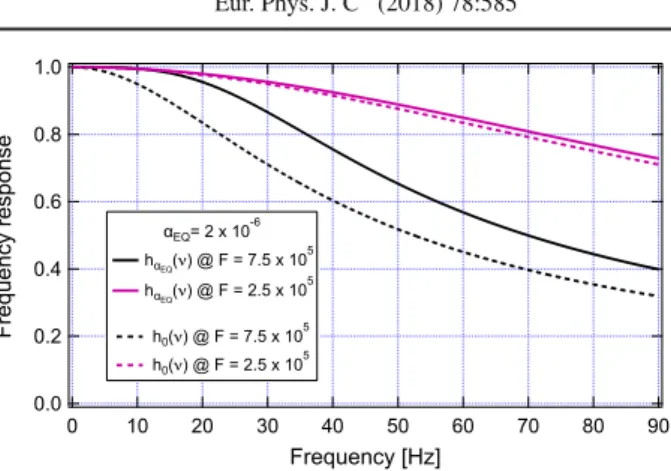
Fig. 4 Comparison of hαEQ(ν)(solid lines) with h0(ν)(dashed lines) for two finesse values and for αEQ= 2 × 10⁻⁶rad. As can be seen the
two functions differ significantly especially at the higher finesse value where N αEQ/2 approaches unity
Although these expressions are rather bulky separately, it can be shown that the ratio of the righthand sides of Eqs. (33)– (32) reduces to the same expression as in the case N αEQ≪ 1:
+
R2sin2α EQ
1− R cos αEQ(2 cos δ− R cos αEQ) ≈ N α2EQ+ / 1 1+2 ν νcut 320 ' 1− N αEQ 2 αEQ ( ≈ N α2EQh0(ν). (34)
Even for N αEQ/2∼ 1 this ratio is proportional to a simple
first order filter h0(ν). We will therefore define a modified
first order filter function hαEQ(ν)from, N k(αEQ)hαEQ(ν)
= +
4[1 − R cos αEQ(2 cos δ− R cos αEQ)] 4
1+ R2− 2R cos(αEQ− δ)5 41+ R2− 2R cos(αEQ+ δ)5
(35) and in Eqs. (30) and (31) we can therefore make the substi-tutions, k(αEQ)h0(ν)→ k(αEQ)hαEQ(ν), (36) k(αEQ)H0(ν)N αEQ 2 → k(αEQ)hαEQ(ν) N αEQ 2 h0(ν). (37) In Fig.4we report the comparison of h0(ν)with hαEQ(ν)
for two different values of N αEQ
2 : 0.50 and 0.17. Given that
our values of N αEQ/2, as we will see below, are close to the
values reported in the Fig.4, to correctly interpret our noise spectra the more general expression of hαEQ(ν)mustbe used.
With all these considerations the measured values for 'measand ,measas a function of '0, ,0and αEQare finally,
'meas= k(αEQ)hαEQ(ν) / '0− N αEQ 2 ,0h0(ν) 0 (38) ,meas= k(αEQ)hαEQ(ν) / ,0+ N αEQ 2 '0h0(ν) 0 (39) where the ratio,
,meas 'meas 1 1 1 1 ,0=0 = N α2EQh0(ν) (40)
gives a direct value for αEQ. The same is true in the presence
of an effect generating a pure rotation ('0 = 0) in which
case, 'meas ,meas 1 1 1 1' 0=0 = −N α2EQh0(ν). (41)
These last four Eqs. (38)–(41) will be used when analysing our data in what follows.
3.3 Noise studies
By studying the noise spectra in ellipticity and rotation and the Cotton-Mouton and Faraday signals one can understand whether the noises S'(ν)and S,(ν)are proportional to N or
not and therefore if they originate from inside or outside of the cavity. Moreover by comparing the measured ellipticity noise S'meas(ν)with the measured rotation noise S,meas(ν)one can
determine whether they are dominated by an ellipticity noise S'(ν)or a rotation noise S,(ν).
Since the measured noise both in ellipticity and in rotation is significantly greater than the expected noise, we assume independent contributions by both ellipticity and/or rota-tion noises, S'meas(ν)and S,meas(ν), generated and
ampli-fied inside the cavity. Hence we use, for the noise densities, the same expressions (38) and (39) used for the signals. We therefore model the measured spectral noise densities as,
S'meas(ν)= k(αEQ)hαEQ(ν) × 6 7 7 8S'(ν)2+ !N α EQ 2 S,(ν)h0(ν) "2 + 9 Se k(αEQ)hαEQ(ν) :2 , (42) S,meas(ν)= k(αEQ)hαEQ(ν) × 6 7 7 8S,(ν)2+ !N α EQ 2 S'(ν)h0(ν) "2 + 9 Sr k(αEQ)hαEQ(ν) :2 , (43) where S'(ν) = Nsψ(ν)and S,(ν) = Nsφ(ν)are
respec-tively the ellipticity and the rotation spectral densities and
where we have added white noise contributions Srand Seto
S,meas(ν)and S'meas(ν)respectively.
4 Measurements
Let us remind the reader that the aim of the present work is to study the signal-to-noise ratio in the PVLAS apparatus as a function of the finesse of the Fabry–Perot cavity. To reduce the finesse of the cavity we have introduced controlled extra losses p to the Fabry–Perot cavity. Given the transmittance T and the intrinsic losses p0of the mirrors, p will cause the
finesse F and the output intensity I0to change according to,
F ( p)= π T+ p0+ p (44) I0(p) Iin = / T T+ p0+ p 02 = /T F (p) π 02 . (45)
In the case of the PVLAS cavity, the best finesse mea-sured was F ≈ 7.7 × 10⁵with a 25% transmission [18],
corresponding to p0= (1.7 ± 0.2) ppm and a transmittance
of each mirror (assumed to be equal) T = 2.4 ± 0.2 ppm. Therefore an extra loss p ≈ 0 ÷ 10 ppm will change the finesse from F = 7.7 × 10⁵to F= 2.5 × 10⁵.
To introduce these extra losses we have used one of the manual vacuum gate valves present in front of the output mirror to clip the Gaussian mode between the mirrors. With a width r0of the intensity profile of the Gaussian mode and
therefore σ = r0
2, clipping at (4.5− 5)σ level is sufficient
to achieve the desired losses p. An estimate can be made considering a circular aperture of radius a. The power loss per pass of the beam inside the cavity is,
p≈ e−2w2a2 = e− a2
2σ 2. (46)
With a ratio x = a/σ = 4.8 the resulting extra losses are p = 10 ppm. Given the relatively large value of x, these extra power losses are therefore obtained without signifi-cantly altering the Gaussian beam profile. It is also true, though, that very small position variations of the gate valve with respect to the beam generate significant variations of the finesse. We have observed that, with the valve inserted, the stability of the finesse is of the order of 1%. In our mea-surements this is the dominant uncertainty factor.
Note also that even if the noise is generated within the whole thickness of the reflecting layers, the physical struc-tures of the multilayer dielectric mirrors corresponding to the highest and the lowest finesses used would differ by no more than a pair of dielectric layers [35]; this justifies the use of an extra loss located outside the mirrors as a means to study the intrinsic birefringence noise of the mirrors as a function of the finesse.
0.01 2 3 4 5 6 7 0.1 2 Intensity [a.u] 0.010 0.008 0.006 0.004 0.002 Time [s] F1 = 688000 F2 = 572000 F3 = 481000 F4 = 383000 F5 = 317000 F6 = 256000 Fit to F6
Fig. 5 Intensity decay curves for the six different positions of the gate
valve clipping the beam to increases the losses inside the cavity. F1–F6 represent the relative finesse values. As an example, an exponential fit is superimposed to the curve relative to F6
Since a reduction by a factor 3 of the finesse results in a factor 9 reduction at the output of the cavity and given that the output power is I∥ = T Icav this also means a factor 9
reduction of the power on the mirrors. We therefore chose to change the input power to the cavity so that at each finesse the output power was the same during all measurements: we chose I0= 0.7 mW.
The theoretical sensitivity for I0= 0.7 mW was already
shown in Fig.2. Superimposed is also the measured sensi-tivity between 10 and 20 Hz with a modulation η0= 10−2.
This measured sensitivity does not change by increasing or decreasing the output power by a factor ten.
During our measurements the magnets were kept in rota-tion at two different frequencies, να= 4 Hz and νβ = 5 Hz
generating Cotton-Mouton peaks at twice these frequencies due to the presence of Argon gas at 850 µbar. The frequency of the Faraday rotation signal induced on the input mirror using an external solenoid was chosen to be νF= 19 Hz.
Six different values of the finesse were chosen for the mea-surements, each separated by approximately 20%. For each finesse value we first measured in the ellipticity configura-tion and then in the rotaconfigura-tion configuraconfigura-tion by inserting the quarter-wave plate. The finesse was determined by measur-ing the intensity decay exitmeasur-ing the cavity after unlockmeasur-ing the laser at the end of each series of measurements.
The intensity decay graphs for the six positions of the gate valve, resulting in the six finesse values used during the measurements, are shown in Fig. 5. These correspond respectively to,
F = (6.88, 5.72, 4.81, 3.83, 3.17, 2.56) × 105, (47) with a 1% uncertainty.
The main goal of the present work is to show whether the noise present in the two configurations of the polarimeter is dominated by an ellipticity noise generated by a fluctuat-ing birefrfluctuat-ingence inside the cavity, i.e. whether it is
multi-10-11 10-9 10-7 10-5 Ellipticity 20 15 10 5 0 Frequency [Hz] Ellipticity spectrum 10-11 10-9 10-7 10-5 Rotation 20 15 10 5 0 Frequency [Hz] Rotation spectrum
Fig. 6 Ellipticity (top panel) and rotation (bottom panel) raw spectra
for an integration time of t = 512 s forF1= 6.88 × 10⁵. In red is
the FFT of the in-phase component whereas in black is the quadrature component. A zoom from 0 Hz to 20 Hz is shown to better appreciate the peaks at 2να = 8 Hz, 2νβ = 10 Hz, of equal amplitudes, and
at νF = 19 Hz. Peaks at να and νβ are also present due to a slight
non orthogonality between the beam and the magnetic field direction generating a time dependent Faraday rotation in the Argon gas
plied by the gain factor N of the Fabry–Perot. To accomplish this, for each finesse value we first determined the value of αEQfrom Eqs. (40) and (41) for both the Faraday and the
Cotton-Mouton measurements. The dependence of both the Cotton-Mouton and Faraday signals are expected to follow the relations given in Eqs. (38) and (39). We have then stud-ied the signal-to-noise ratios of the various signals both in the rotation and in the ellipticity configurations to study their behaviour as a function of the finesse.
5 Results and discussion
Typical raw ellipticity (top) and rotation (bottom) spectra measured in a time t = 512 s at the highest finesse of F1 = 6.88 × 10⁵are shown in Fig.6. Data sampling was
performed at 256 Hz resulting in spectra with a frequency resolution of !νres= 1.5 × 10⁻⁵Hz. In both the ellipticity
and rotation channels the Argon Cotton-Mouton signals at 2να= 8 Hz and 2νβ = 10 Hz are clearly visible, with equal
amplitudes due to identical magnets, along with the Faraday rotation signal at νF = 19 Hz induced in the input mirror
of the cavity. The small sidebands around 2να,β are due to
2.5x10⁻⁶ 2.4 2.3 2.2 2.1 2.0 αEQ [rad] 5x10⁵ 4 3 2 1 0 Number of passes αEQ @ 8Hz αEQ @ 10Hz αEQ @ 19Hz
Fig. 7 Determination of αEQas a function of N for both the
Cotton-Mouton signals at 2να,βand for the Faraday rotation at νF
generated by the driving system of the magnets. The ampli-tude error on the main peaks due to these sidebands is less than 1 ‰. In both panels of the Fig.6one can also distin-guish two peaks at να = 4 Hz and νβ = 5 Hz due to a small
component of the magnetic field along the beam direction generated by a small non orthogonality of the magnetic field with respect to the beam propagation direction. This small component of the magnetic field generates a Faraday rotation in the gas inside the cavity. Indeed these peaks are higher in the rotation spectrum. A small Faraday effect is also gener-ated in the mirrors due to the stray field but this rotation is negligible with respect to the rotation generated in the gas.
Notice how in the rotation spectrum the integrated noise and the two Cotton-Mouton signals are smaller with respect to the ellipticity spectra whereas the Faraday signals are larger.
In Fig. 6 we have also reported (in black) the quadra-ture demodulation spectra integrated over the same time t. This integrated noise corresponds to a peak spectral density of Squad = 1.6 × 10⁻⁸/√Hz, in agreement with the
sen-sitivity, shown in Fig.2, due to noise sources independent of ellipticity such as shot-noise, Johnson noise, diode dark current noise and laser relative intensity noise considering I0= 0.7 mW and η0= 10−2. This noise is the same in both
the ellipticity and the rotation spectra. The in-phase noise is clearly of a different origin. Small peaks, less than 1% of the in-phase peaks, are present in the quadrature channel which are consistent with a phase error in the demodulation of about 1◦.
5.1 Determination of αE Q
For each value of the finesse we have first determined the value of αE Q, necessary to evaluate the true ellipticities and
rotations due to the Cotton-Mouton and Faraday effects, according to Eqs. (40) and (41). In Fig.7we have plotted the values of the ratios,
,meas 'meas 2 N h0(ν) 1 1 1 1 ν=8 Hz,10 Hz= α EQ, (48)
at 8 and 10 Hz as a function of the number of passes N = 2Fπ and 'meas ,meas 2 N h0(ν) 1 1 1 1ν=19 Hz= αEQ. (49)
Since αEQis a property of the mirror coatings it is
indepen-dent of N , as expected. The average value for αEQat 8 and
10 Hz is
αEQ|ν=8 Hz,10 Hz= 2.30 × 10⁻⁶rad
σαEQ|ν=8 Hz,10 Hz= 2 × 10⁻⁸rad (50)
where σαEQis the standard deviation obtained from the
plot-ted data. This value is consistent with the statistical error of each single measurement.
The same can be done by considering the measured rota-tion and ellipticity peaks at ν= 19 Hz:
αEQ|ν=19 Hz= 2.35 × 10⁻⁶rad
σαEQ|ν=19 Hz= 6 × 10⁻⁸rad (51)
Here the standard deviation σαEQ|ν=19 Hz obtained from
the plotted data is significantly larger than the statistical error of each data point due to the significantly smaller value of αEQat N = 161000 with respect to the other data points.
Furthermore the average value of αEQ for the data at the
higher finesses is significantly larger than the average value obtained using the Cotton-Mouton effect. There is clearly a small systematic effect when using the Faraday effect by applying a magnetic field on the mirrors which at the moment is not well understood but may be due to the substrate of the mirror. The weighted average of the two values considering the standard deviations reported in (50) and (51), which we will use in the following, is αEQ = 2.305 × 10⁻⁶ rad with
standard deviation σαEQ= 2 × 10⁻⁸rad.
5.2 Cotton-Mouton and Faraday signals in the ellipticity channel versus N
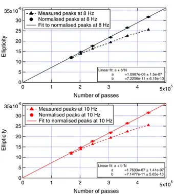
In Fig.8we have plotted the peak amplitudes 'measof the
ellipticity signals at 8 and 10 Hz as a function of N . In the same figure we have also plotted the values of '0obtained
from Eq. (38) taking into account the frequency dependence hαEQ(ν) of the signals and the amplitude reduction due to
k(αEQ). As expected these lie on a line passing through the
origin indicating that indeed the signal is '0= Nψ0. The
slope of the lines give the value of the ellipticity per pass ψ0= (7.20 ± 0.04) × 10−11acquired by the light resulting
in a Cotton-Mouton constant [36] !nu= !n/B2= (5.63±
35x10-6 30 25 20 15 10 5 0 Ellipticity 5x10⁵ 4 3 2 1 0 Number of passes Measured peaks at 8 Hz Normalised peaks at 8 Hz Fit to normalised peaks at 8 Hz
Linear fit: a + b*N a =1.0987e-08 ± 1.5e-07 b =7.2256e-11 ± 6.15e-13 35x10-6 30 25 20 15 10 5 0 Ellipticity 5x10⁵ 4 3 2 1 0 Number of passes Measured peaks at 10 Hz Normalised peaks at 10 Hz Fit to normalised peaks at 10 Hz
Linear fit: a + b*N
a =1.7633e-07 ± 1.41e-07 b =7.1477e-11 ± 5.65e-13
Fig. 8 Measured Cotton-Mouton peaks at 2να(top) and 2νβ(bottom)
as a function of N . The experimental points connected with dashed lines are not corrected for the cavity response. The dots lying on the linear fit are the experimental values corrected for the cavity response. The two slopes are compatible within their errors
4x10⁻⁶ 3 2 1 0 Ellipticity 5x10⁵ 4 3 2 1 0 Number of passes Parabolic fit: a*N + b*N2
a =-7.4099e-14 ± 1.76e-13 b =2.264e-17 ± 4.94e-19 Measured ellipticity peaks at 19 Hz
Normalised peaks at 19 Hz Fit to normalised peaks at 19 Hz
Fig. 9 Measured Faraday peak at νF in the ellipticity channel as a
function of N . The experimental points connected with dashed lines are not corrected for the cavity response. The dots lying on the parabolic fit are the experimental values corrected for the cavity response
In Fig.9we have plotted the values of 'measof the
ellip-ticity at 19 Hz. This signal is due to the Faraday rotation being transformed into ellipticity because of the birefrin-gence of the cavity. In the same figure we have also plotted the values of N2 αEQ
2 φ0, obtained having normalised the
val-ues 'measfor the response of the polarimeter, as a function of Naccording to the expression deduced from Eq. (38) having set '0= 0:
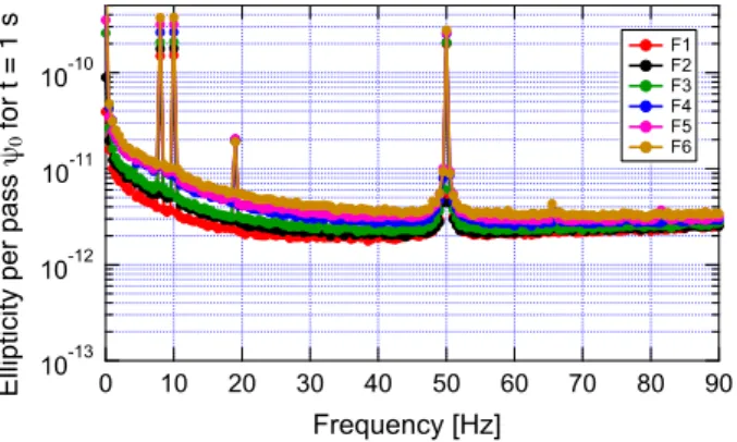
Fig. 10 Ellipticity spectra for the six finesse values rescaled to a 1 s
integration time. The raw spectra have been rebinned by taking rms averages of the raw spectra in 0.5 Hz frequency intervals. The peak at 50 Hz is due to the mains
1 1 1 1 1 'meas h0(ν)hαEQ(ν)k(αEQ) 1 1 1 1 119 Hz= N αEQ 2 ,0= N 2αEQ 2 φ0. (52) As expected from this last equation these values lie on a parabolic curve allowing the determination of the rotation per pass φ0= (1.96± 0.04)×10−11rad/pass. It is estimated that
the contribution of the substrate is less than 1%, compatible with the parabola passing through the origin within the errors. 5.3 Ellipticity noise versus N
In Fig.10one can see the ellipticity rms spectra at the six different finesse values, where the raw spectra have been rebinned in 0.5 Hz frequency bins.
These spectra have not been normalised for the amplifica-tion factor N and frequency response k(αEQ)hαEQ(ν)given
by Eq. (32). As can be seen not only do the Cotton-Mouton ellipticity signals and the peaks at νF= 19 Hz decrease with
decreasing N , as already discussed, but so does the noise. By normalising each spectrum with the cavity response given by Eq. (38) and assuming the noise to be dominated by the intra-cavity ellipticity noise sψ(sφ = 0 and Se = 0) in Eq. (42),
one finds the plot shown in Fig.11. In this figure, all the noise components of the spectra lie on a common curve (except for a small broad structure between 5 and 10 Hz at the lower finesse values). The Cotton-Mouton peaks also indicate a common value whereas the signal at νFdoes not, as expected.
Instead, by normalising the noise spectra assuming an intracavity rotation noise sφ(sψ= 0 and Se= 0) in equation
(42), one obtains the plots in Fig.12. In this case the peaks at νF, which have an origin from a Faraday effect, overlap
whereas the noise and the Cotton-Mouton peaks do not. It is also apparent that the noise does not behave as an intracavity rotation noise sφ.
Fig. 11 The six ellipticity spectra of Fig.10rescaled assuming an ellip-ticity noise S'proportional to N and taking into account the frequency
response of the cavity
Fig. 12 The six ellipticity spectra of Fig.10rescaled assuming a rota-tion noise S,proportional to N and taking into account the frequency
response of the cavity
In Fig.13we report the signal-to-noise ratios for both the Cotton-Mouton signals at 2να = 8 Hz (purple) and 2νβ =
10 Hz (green) extracted from Fig.10. On the same plot we have also reported the ratio of the Cotton-Mouton signal at 2νβ = 10 Hz with respect to the noise at 20, 30, 40 and
90 Hz to see whether indeed the noise is independent of the finesse also at higher frequencies. The value of the noise at 8 and 10 Hz is determined as the average of the noise on either side of the peaks in a frequency range of 0.5 Hz. For the other frequencies the noise is determined as the average over a 0.5 Hz frequency range.
As can be seen, the ratios at 8 and 10 Hz are indeed inde-pendentof the finesse. The apparent increase of the signal-to-noise ratio with N at higher noise frequencies is actually only due to the different frequency response of the cavity at the frequency of the signal and at the frequency of the noise. Following the hypothesis that the noise in the polarimeter is dominated by an ellipticity noise per pass sψwe have fitted
the different signal-to-noise ratios with the expression,
2 3 4 5 6 100 2 3 4 5 6 1000 2
Signal to noise ratio [t = 1 s]
400x103 350 300 250 200 Number of passes N Signal to noise ratios with respective fits superposed
Sig 8 Hz, noise 8 Hz Sig 10 Hz, noise 10 Hz Sig 10 Hz, noise 20 Hz Sig 10 Hz, noise 30 Hz Sig 10 Hz, noise 40 Hz Sig 10 Hz, noise 90 Hz
Fig. 13 Signal-to-noise ratios of the Cotton-Mouton peaks with
respect to the noise at different frequencies. The fits take into account the cavity response at the different frequencies according to Eq. (53)
'meas(νsig) S'meas(νnoise) = hαEQ(νsig) hαEQ(νnoise) ψ0 sψ(νnoise), (53) obtaining the superimposed fits.
Considering the more complicated expression (42) in which one fixes a common ellipticity noise per pass sψ, a
common rotation noise per pass sφfor each value of N and
a flat baseline noise contribution Seaccording to the
expres-sion, 'meas(νsig) S'meas(νnoise) = hαEQ(νsig)ψ0 . sψ(νnoise)2+ 2N α EQ 2 sφ(νnoise)h(νnoise) 32 + S2e N k(αEQ)hαEQ(νnoise) , (54) does not improve the quality of the fitted data estimated using χndf2 . A global fit considering all the data in Fig.13gives the following limits: sφ/sψ<0.4 and Se<2× 10−81/√Hz.
The noise therefore behaves as an ellipticity noise sψ
gen-erated within the cavity and multiplied by a factor N , just like the Cotton-Mouton signals: the total noise S' = Nsψis
proportional to the number of passes N . We therefore con-clude that the dominating noise source at frequencies up to ν= 90 Hz is due to a pure ellipticity noise generated in the dielectric coatings of the cavity mirrors.
By rescaling Fig.11to obtain an optical path difference sensitivity one finds the graph in Fig.14.
Fig. 14 The six ellipticity spectra of Fig.11rescaled to show the com-mon optical path difference sensitivity independent of the number of passes N assuming an ellipticity noise S'proportional to N and taking
into account the frequency response of the cavity
Fig. 15 Rotation spectra for the six finesse values rescaled to a 1 s
integration time. The raw spectra have been rebinned by taking rms averages of the raw spectra in 0.5 Hz frequency intervals
5.4 Ellipticity noise versus rotation noise
In the previous section we have discussed the ellipticity spec-tra for the six finesse values. In Fig.15we report the respec-tive rotation spectra.
Two facts are apparent: the rotation noise is smaller than the ellipticity noise at all frequencies for corresponding finesse values; the noise spectra in rotation flatten above about 40 Hz at the lower finesse values. This noise floor results to be Sr = 3.2×10⁻⁸/√Hz with a dispersion around
Srof σSr = 0.2×10⁻⁸/ √
Hz. This noise is slightly above the quadrature noise which corresponds to the intrinsic rotation noise of the polarimeter.
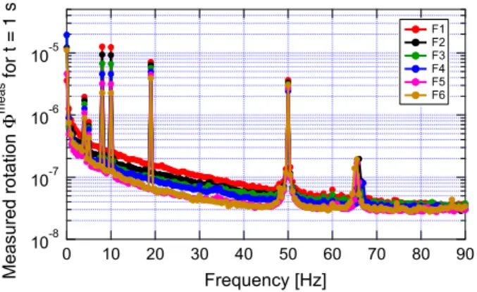
To further confirm that the dominant noise source orig-inates from a birefringence fluctuation we have considered the ratios of the noise spectrum in ellipticity with respect to the noise spectrum in rotation for the six different finesse values. These spectra have been fitted with the expressions (42) and (43),
Fig. 16 Plots of the ratios of the ellipticity noise to the rotation noise.
Fits are taken from 20 and 90 Hz. The peak frequencies have been excluded in the fits. See text for details
S'meas(ν) S,meas(ν) = . sψ(ν)2+ 2N α EQ 2 sφ(ν)h0(ν) 32 + Se2 N k(αEQ)hαEQ(ν) . sφ(ν)2+ 2N α EQ 2 sψ(ν)h0(ν) 32 + Sr2 N k(αEQ)hαEQ(ν) , (55) where we have used a frequency dependence of sψ(ν) =
)
(aν−1)2+ (bν−0.25)2as a result of fitting Fig.11, from
10 to 90 Hz, and we have assumed that the ratio sφ/sψ is
independent of frequency. The fit of the ratio of the noises using Eq. (55) has been performed from 20 to 90 Hz and the frequencies at which a peak is present have been excluded. With these assumptions we obtain the global fits shown in Fig.16in which the free parameters are the ratio sφ/sψand
Seand the fixed value of Sr = 3.2 × 10⁻⁸/√Hz was used as
deduced from Fig.15above 40 Hz. The fits indicate a ratio sφ/sψ = (0.21± 0.01) and Se≤ 3×10⁻⁸/√Hz compatible with the shot noise limit shown in Fig.2. On the same graphs we have also plotted the two cases for sφ/sψ = 0 (dashed
green) and sφ/sψ = 1 (dashed blue) keeping the values for
Seas obtained from the global fit and Sr = 3 × 10⁻⁸.
These results confirm our interpretation of the noise mea-surements: the observed noise is dominated by an ellipticity noise generated by a birefringence inside the cavity. Rotation noise plays only a minor role.
5.5 Consequences of results
A first important consequence of the findings presented in this section is that the signal-to-noise ratio in a Fabry–Perot based polarimeter with a calculated optical path difference
sensitivity equal to or better than the sensitivity shown in Fig. 14 will not improve by increasing the finesse of the cavity. Assuming a predicted shot noise sensitivity given by Eq. (14), the maximum useful finesse up to which one gains in signal to noise ratio is determined by,
Fmax=. e
I∥q λ
2S!D, (56)
where S!D can be read off Fig.14. For the experimental configuration presented in this paper, where S!D ≈ 6 × 10⁻¹⁹m/√Hz @10 Hz, one finds Fmax= 1.6 × 10⁴.
The second important fact resulting from these measure-ments is that the dominant source of noise is indeed due to a birefringence fluctuation in the cavity mirror coatings.
6 Noise origin
Polarimetric measurements using a Fabry–Perot cavity to increase the effective optical path length have reached an intrinsic limit due to the coatings of the cavity mirrors. Our measurements show that this noise is due to birefringence fluctuations in the coatings which we believe are of thermal origin.
As mentioned in Sect.3.1cavity mirrors always present an intrinsic birefringence. There could therefore be two princi-pal causes for these birefringence fluctuations: a fluctuation of the intrinsic birefringence; a fluctuation of the birefrin-gence independent of the intrinsic value. As was shown in Fig.3, there is a very strong correlation in the optical path difference noise between completely different experiments with very different values of F . This seems to indicate that the source of the intrinsic birefringence noise is independent of the intrinsic mirror birefringence inducing the retardations α1,2. This hypothesis seems confirmed by the estimation of
the thermo-refractive noise in Sect.6.1.
We also note that any polarization effect intrinsic to the cavity, be it static or dynamical, is generated in the first reflecting layers encountered by the light from inside the cavity. With a transmittance of the mirrors T = 2.4 × 10⁻⁶, as is the case of the PVLAS experiment [18], the electric field inside the reflective coatings has an exponential decay with,
NLP
λLP = − ln
√
T , (57)
where NLP≈ 20 is the total number of high refractive index
- low refractive index pairs composing the reflective coating and λLPrepresents the number of coating pairs after which
the electric field (as opposed to the intensity) has decreased to 1/e of the incident field. One finds λLP = 3.0. Most of
the ellipticity (signal and noise) is therefore accumulated in
the first λLPpairs of dielectric coatings for each reflection.
This corresponds to a geometrical thickness dLP ≃ 1 µm.
These considerations further justify the use of an extra loss located outside the mirrors as a means to study the intrinsic birefringence noise of the mirrors.
There are three possible causes for birefringence thermal noise in a medium: direct temperature dependence of the index of refraction (thermo-refractive effect); indirect tem-perature dependence of the index of refraction due to a linear expansion coefficient coupled to a stress optic coefficient; volume fluctuations due to Brownian motion. Here we will only discuss the first two effects.
A lot of literature (see for example [38–41] exists which deals with the phase noise induced in interferometric grav-itational wave antennas by thermal fluctuations of mirrors (coating, substrate). Indeed the main concern in their case are length variations in the incident direction. Very little (if none) exists for what concerns the effect of fluctuations in the plane of the mirror surfacecausing birefringence. In the following we will try to estimate this effect.
6.1 Thermo-refractive effect
Let us consider the indeces of refraction of the mirror coatings along the natural axes of a mirror as n∥and n⊥ resulting in a birefringence !n= n∥− n⊥. The optical path through the coating of a mirror per reflection for light polarised parallel and perpendicularly to the slow axis (here considered to be the∥ direction) will be,
D∥ ≈ 2 & dLP n∥dl (58) D⊥ ≈ 2 & dLP n⊥ dl (59)
where the factor 2 is intended to take into account the round trip inside the coating. The intrinsic optical path difference of a mirror coating per reflection will therefore be,
!D = D∥− D⊥ ≈ 2
&
dLP
!n dl. (60)
By considering the thermo-refractive effect due to a tem-perature dependence of n= n(T), the optical path difference temperature dependence will be,
d!D(T) dT ≈ 2 & dLP d!n(T) dT dl. (61)
Hence d!D(T)/dT̸= 0 only if dn∥/dT̸= dn⊥/dT. In this
case the optical path difference spectral density S!D(ν)due to the thermo-refractive effect will be,
S!D(ν)= d!D(T)
dT ST(ν), (62)
where ST(ν)is the temperature noise spectral density.
An estimate of !D due to the intrinsic mirror birefrin-gence can be obtained from the value of αEQ = 2.3 ×
10−6rad, resulting in, !D≈ 2
&
dLP
!n dl= αEQ
2π λ≈ 4 × 10⁻¹³m. (63) A rough value for !1nd!ndT ∼ 10−5K−1for fused silica can
be deduced from the expressions reported in [37] considering n∥≃ n⊥. Therefore, d!D dT =2 & dLP d!n dT dl∼ 10−5 ×2 & dLP !n dl∼ 4 × 10⁻¹⁸ m K. (64)
Following Ref. [38] the temperature fluctuations averaged over a volume πr2
0dLP/2 occupied by the Gaussian power
profileof waist r0being reflected using a weight function
q(r), q(r) = 2
πr02dLP
e−,x2+y2-/r02 e−2z/dLP, (65)
results in a temperature noise spectral density ST(ν)[38],
ST2(ν)= √ 2κBT2 πr02√2πνρCTλT = √ 2kBT2 2πνρCTrT3 r2 T πr02, (66) where κBis the Boltzmann constant, ρ is the density, CTis
the specific heat capacity, λTis the thermal conductivity and,
rT=
+ λT
ρCT2πν, (67)
is the characteristic diffuse heat transfer length (dLP≪ rT≪
r0). In Eq. (66) the ratio rT2/r02represents the inverse of the
number of unit spheres of radius rT covering the beam of
radius r0thereby averaging out the temperature fluctuations.
Considering fused silica (FS), for which ρ = 2200 kg/m3,
CT= 670 J/(kg K) and λT= 1.4 W/(m K) this results in,
STFS(ν)≃ 2 × 10⁻⁸ √K
Hz @ 1 Hz, (68)
having set the beam diameter r0 ≈ 0.5 mm. Considering
tantala, Ta2O5, (TA) instead (we are assuming this is the
material used for the high-index layer in the mirror coating),
for which ρ= 8200 kg/m3, CT= 300 J/(kg K) and λT =
[0.026÷ 15] W/(m K) (for a film) [42], one finds, STAT (ν)≃ (1 ÷ 6) × 10−8 √K
Hz @ 1 Hz. (69)
With the above values the thermo-refractive noise spectral density in optical path difference S!TRD(ν)can be estimated to be of the order, STR!D(ν)= d!D dT + √ 2kBT2rT(ν) πr2 0λT ∼ 10 −25 √m Hz @ 1 Hz, (70) well below the measured values reported in Figs.3and14. We therefore believe that the source of noise in the PVLAS polarimeter is not due to a thermo-refractive effect. 6.2 Stress induced birefringence
Local length fluctuations will generate stress fluctuations leading to birefringence through the stress optic coefficient. Indeed given a stress optical coefficient CSOand a Young’s
modulus Y the induced variation in the index of refraction due to stress is given by,
δn∥,⊥ = CSOY !δl ∥,⊥ l " , (71)
where δl∥,⊥/lis a relative length variation along two perpen-dicular directions∥ and ⊥ over a lengthl. Again following the considerations in Ref. [38] an order of magnitude estimate of the induced birefringence noise spectral density S!n(ν)
over the spot size of the reflected beam due to temperature fluctuations related to stress can be made.
The average relative length fluctuations of δrT
rT over the
spot surface, indicated by the brackets⟨⟩∥,⊥ where∥ and ⊥ indicate two perpendicular directions, will be,
;δr T rT < ∥,⊥ = αT ST(ν)= αT + √ 2κBT2 πr2 0√2πνρCTλT , (72)
where αTis the linear expansion coefficient. This will
gen-erate a birefringence noise spectral density, S!n(ν)≃ CSOY 6 7 7 8;δrT rT <2 ∥+ ;δr T rT <2 ⊥ = CSOY αT + 2√2κBT2 πr2 0√2πνρCTλT . (73)
A very rough estimate of the optical path difference spec-tral density noise S!D = 2%d
LPS!ndl accumulated in a
S!D≈ 2S!ndLP= CSOY αTdLP r0 + 8T2κB π√π νρCTλT. (74)
For fused silica for which αT= 5 × 10⁻⁷K−1, Y= 70 GPa
and CSO= 3 × 10⁻¹²Pa−1one finds,
S!DFS ∼ 7 × 10⁻²¹ √m
Hz@ 1 Hz (75)
whereas for tantala,
S!DTA ∼ (1 ÷ 6) × 10−19 √m
Hz @ 1 Hz (76)
where the values for tantala are Y = 150 GPa and αT =
8× 10⁻⁶ K−1 and we have use CSO = 3 × 10⁻¹² Pa−1
for fused silica not having found a value for tantala in the literature. Generally it is found in literature that CSO is∼
(10−12÷ 10−11) Pa−1 with a particularly large value for
Nb2O5 with CSO = 95 × 10−12 Pa−1 [43]. These values
justify our approximation. The value for STA
!D in the case of tantala is quite close
to the measured values especially at higher frequencies. The exact expression for S!D is beyond the scope of this paper but indeed a stress mechanism could generate a birefringence noise of the same order of magnitude as the one measured.
This stress will be present both in the substrate and in the mirror coatings. As discussed above, given that the electric field within the coating is strongest in the first λLP layers
encountered by the light in the cavity, the induced S!D will be dominated by these first layers and in particular by the tantala layers.
7 Conclusions
Birefringence noise of the Fabry–Perot cavity limits the sen-sitivity of precision measurements in polarimeters like those designed to detect the birefringence of vacuum due to mag-netic fields. We have measured the noise present in the PVLAS polarimeter in both ellipticity and rotation modes along with Cotton-Mouton and Faraday signals as a func-tion of the finesse of the Fabry–Perot cavity. We have shown that the signal-to-noise ratio of the Cotton-Mouton ellipticity signals is independent of the finesse of the cavity as is the ellipticity noise. We have shown that for the rotation noise this is not the case. We have also studied the ellipticity noise to rotation noise ratios which confirm that the dominant noise source in the polarimeter is a fluctuating birefringence inside the Fabry–Perot cavity.
We note that the noise is generated in the first few layers of the mirror coatings and we infer that, with an order of magnitude estimation, the origin could be due to thermally
induced stress fluctuations namely due to a thermo-elastic effect.
It is therefore apparent that the continuous search to improve the sensitivity in optical path difference S!D by increasing the finesse of the Fabry–Perot cavity has reached a limit.
The quest to measure vacuum magnetic birefringence using optical techniques must therefore,
– reduce the optical path difference noise by cooling the mirrors and/or by finding new materials for the coatings with a lower stress optic coefficient and/or lower linear expansion coefficient;
– decrease the number of reflections (finesse) and increase the cavity and magnetic field lengths to preserve the opti-cal path length.
– increase the vacuum magnetic birefringence signal using high, long, static superconducting fields and inducing the necessary signal modulating for improved sensitivity by varying the polarisation [44,45].
Finally let us note that if the intrinsic total retardationN αEQ 2
can be kept low in such a way that the mixing between ellip-ticity and rotation is also small, then increasing the finesse during rotation measurements is advantageous. Indeed given that the dominant source of ellipticity noise is due to bire-fringence fluctuations, rotation sensitivity may not be limited by an intrinsic thermal source. This could lead to improved laboratory experimental limits on the existence of axion like particles [19,23,24,46].
Open Access This article is distributed under the terms of the Creative
Commons Attribution 4.0 International License (http://creativecomm ons.org/licenses/by/4.0/), which permits unrestricted use, distribution, and reproduction in any medium, provided you give appropriate credit to the original author(s) and the source, provide a link to the Creative Commons license, and indicate if changes were made.
Funded by SCOAP3.
References
1. H. Euler, B. Kockel, Naturwiss 23, 246 (1935) 2. H. Euler, Ann. Phys. (Leipzig) 26, 398 (1936) 3. W. Heisenberg, H. Euler, Z. Phys. 98, 714 (1936)
4. V.S. Weisskopf, K. Dan. Vidensk. Selsk. Mat Fys. Medd. 14, 6 (1936)
5. R. Karplus, M. Neuman, Phys. Rev. 80, 380 (1950) 6. J. Schwinger, Phys. Rev. 82, 664 (1951)
7. G.V. Dunne, Int. J. Mod. Phys. A 27, 1260004 (2012) 8. T. Erber, Nature 4770, 25 (1961)
9. R. Baier, P. Breitenlohner, Acta Phys. Austriaca 25, 212 (1967) 10. R. Baier, P. Breitenlohner, Nuovo Cimento 47, 117 (1967) 11. Z. Bialynicka-Birula, I. Bialynicki-Birula, Phys. Rev. D 2, 2341
(1970)
13. F. Della Valle et al. (PVLAS collaboration), Phys. Rev. D 90, 092003 (2014)
14. R. Rosenberg, C.B. Rubinstein, D.R. Herriott, Appl. Opt. 3, 1079 (1964)
15. P. Pace, Studio e realizzazione di un ellissometro basato su una cavità Fabry-Perot in aria nell’ambito dell’esperimento PVLAS, Laurea Thesis, University of Trieste (1994) (unpublished) 16. D. Jacob et al., Appl. Phys. Lett. 66, 3546 (1995) 17. G. Zavattini et al., Appl. Phys. B 83, 571 (2006)
18. F. Della Valle et al. (PVLAS collaboration), Opt. Express 22, 11570 (2014)
19. F. Della Valle et al. (PVLAS collaboration), Eur. Phys. J. C 76, 24 (2016)
20. H.-H. Mei et al. (Q & A collaboration), Mod. Phys. Lett. A 25, 983 (2010)
21. A. Cadène et al. (BMV collaboration), Eur. Phys. J. D 68, 10 (2014) 22. X. Fan et al. (OVAL collaboration), Eur. Phys. J. D 71, 308 (2017) 23. A. Ejlli, Progress towards a first measurement of the magnetic bire-fringence of vacuum with a polarimeter based on a Fabry-Perot cavity, Ph.D. Thesis, University of Ferrara (2017) (unpublished) 24. L. Maiani, R. Petronzio, E. Zavattini, Phys. Lett. B 175, 359 (1986) 25. E. Zavattini et al. (PVLAS collaboration), Phys. Rev. D 77, 032006
(2008)
26. G. Zavattini, E. Calloni, Eur. Phys. J. C 62, 459 (2009) 27. D.V. Martynov et al., Phys. Rev. D 93, 112004 (2016)
28. R. Cameron et al. (BFRT collaboration), Phys. Rev. D 47, 3707 (1993)
29. M. Bregant et al. (PVLAS collaboration), Phys. Rev. D 78, 032006 (2008)
30. F. Della Valle et al. (PVLAS collaboration), N. J. Phys. 15, 053026 (2013)
31. N. Uehara, K. Ueda, Appl. Phys. B 61, 9 (1995) 32. P. Micossi et al., Appl. Phys. B 57, 95 (1993) 33. F. Brandi et al., Appl. Phys. B 65, 351 (1997)
34. A. Ejlli, F. Della Valle, G. Zavattini, Appl. Phys. B 124, 22 (2018) 35. M. Born, E. Wolf, Principles of Optics, 6th edn. (Pergamon Press,
Oxford, 1989)
36. C. Rizzo, A. Rizzo, D. Bishop, Int. Rev. Phys. Chem. 16, 81 (1997) 37. C.Z. Tan, J. Non-Cryst, Solids 238, 30 (1998)
38. V.B. Braginsky, M.L. Gorodetsky, S.P. Vyatchanin, Phys. Lett. A
271, 303 (2000)
39. V.B. Braginsky, M.L. Gorodetsky, S.P. Vyatchanin, Phys. Lett. A
264, 1 (1999)
40. G. Harry, T.P. Bodiya, R. Desalvo, Optical Coatings and
Ther-mal Noise in Precision Measurement(Cambridge University Press, Cambridge, 2012)
41. S. Gras, M. Evans.arXiv:1802.05372v1
42. E. Welsch, K. Ettrich, D. Ristau, U. Willamowski, Int. J. Thermo-phys. 20, 965 (1999)
43. Tei-Chen Chen et al., J. Appl. Phys. 101, 043513 (2007) 44. G. Zavattini, F. Della Valle, A. Ejlli, G. Ruoso, Eur. Phys. J. C 76,
294 (2016)
45. G. Zavattini, F. Della Valle, A. Ejlli, G. Ruoso, Eur. Phys. J. C 77, 873 (2017)
46. S.-J. Chen, H.-H. Mei, W.-T. Ni, Mod. Phys. Lett. A 22, 2815 (2007)