Università degli Studi di Messina
Dipartimento di Scienze Chimiche, Biologiche, Farmaceutiche ed Ambientali
Dottorato di Ricerca in “Scienze Chimiche” Doctor of Philosophy in “Chemical Sciences”
Chromatographic Separation Techniques coupled to Mass Spectrometry for the Analysis of Complex Samples
PhD Thesis of: Supervisor:
Veronica Inferrera Prof. Paola Dugo
Coordinator:
Prof. Sebastiano Campagna
SSD CHIM/10 XXIX Ciclo 2014-2016
Chapter I General Introduction 1.1. Introduction ... 1 1.2. Columns ... 2 1.2.1. Column efficiency ... 3 1.2.2. Resolution ... 5 1.3. Detection ... 6 1.4. General trends ... 7 REFERENCES ... 8 Chapter II Ultra High Pressure Liquid Chromatography 2.1. Introduction ... 9
2.2. UHPLC system requirements ... 12
2.3. Moving a HPLC method to an UHPLC ... 14
2.3.1. Isocratic mode ... 14
2.3.2. Gradient mode ... 15
REFERENCES ... 17
Chapter III Supercritical Fluid Chromatography 3.1. Introduction ... 19
3.3. Stationary phase types ... 25
3.4. Instrumentation ... 27
3.4.1. Towards ultra high performance SFC ... 28
REFERENCES ... 30
Chapter IV Multidimensional Liquid Chromatography 4.1. Introduction ... 33
4.2. Multidimensional chromatography approaches ... 34
4.3. Theoretical concepts: peak capacity, orthogonality and sampling rate ... 36
4.4. Method optimization and instrumentation ... 41
4.4.1. General overview ... 41
4.4.2. First dimension ... 42
4.4.3. Second dimension ... 43
4.4.4. Interface ... 46
4.5. 2D comprehensive SFC-based separations ... 48
4.6. Detectors ... 50 4.7. Data processing ... 51 REFERENCES ... 53 Chapter V Mass Spectrometry 5.1. Introduction ... 57
5.2. Mass resolution and mass accuracy ... 59
5.2.1. Resolution and resolving power ... 59
5.2.2. Mass accuracy ... 60
5.2.3. High-resolution mass spectrometry ... 61
5.3.1. Ion sources ... 62
5.3.2. Mass analyzers ... 65
5.3.2.1. Quadrupole (Q) and Q-based mass analyzers ... 69
5.3.2.2. Time-of-flight ... 70
5.3.3. Detectors ... 73
5.4. Tandem mass spectrometry ... 74
5.5. Ion mobility spectrometry ... 76
5.5.1. Separating ions according to differences in gas-phase structure ... 78
5.5.2. Traveling wave ion mobility spectrometry-mass spectrometry: introduction to Synapt G2-Si HDMS instrument ... 80
REFERENCES ... 83
Chapter VI Lipidomics-type analysis by ultra-high pressure liquid chromatogragraphy – quadrupole mass spectrometry by using ESI and APCI interfaces 6.1. Introduction ... 89
6.2. Experimental section ... 91
6.2.1. Sample and chemicals ... 91
6.2.2. Sample preparation ... 93
6.2.3. Instrumentation and analytical conditions ... 93
6.3. Results and discussion ... 95
6.3.1. UHPLC-Q MS method ... 96
6.3.2. Standard lipids analyzed by UHPLC-Q MS ... 97
6.3.2.1. Polar standards lipids ... 105
6.3.2.2. Non-polar lipids ... 114
6.3.3. Lipidomics analysis of plasma sample by UHPLC-Q MS ... 115
6.4. Conclusions ... 127
Chapter VII
Impact of ultra performance convergence chromatography coupled to time-of-flight mass spectrometry on lipid analysis: applications to triacylglycerol fingerprinting in edible oils
7.1. Introduction ... 131
7.2. Experimental section ... 133
7.2.1. Samples and chemicals ... 133
7.2.2. Instrumentation and analytical conditions ... 134
7.3. Results and discussion ... 135
7.3.1. Optimization of chromatographic conditions ... 135
7.3.2. Chromatographic separation and identification of triacylglycerols ... 136
7.3.3. IMS separation of triacylglycerols ... 144
7.4. Conclusions... 146
REFERENCES ... 147
Chapter VIII Off-line multidimensional convergence chromatography/liquid chromatography-mass spectrometry for characterization of the pigment fraction in sweet bell peppers (Capsicum annuum L.) 8.1. Introduction ... 149
8.2. Experimental section ... 151
8.2.1. Chemicals ... 151
8.2.2. Samples and sample preparation ... 152
8.2.3. Instrumentation and software ... 153
8.2.4. Analytical conditions ... 153
8.2.5. Statistical analysis ... 156
8.3. Results and discussion ... 156
8.4. Conclusions... 175
Chapter IX
On-line coupling of ultra performance convergence chromatography and ultra high pressure liquid chromatography for enhancing orthogonality in comprehensive separations
9.1. Introduction ... 177
9.2. Experimental section ... 178
9.2.1. Chemicals ... 178
9.2.2. Sample and sample preparation ... 179
9.2.3. Instrumental set-up ... 179
9.2.4. Analytical conditions ... 180
9.2.5. Software ... 182
9.3. Results and discussion ... 182
9.4. Conclusions ... 188
REFERENCES ... 188
Chapter X Multidimensional preparative liquid chromatography to isolate flavonoids from Citrus products 10.1. Introduction ... 189
CASE 1. 10.2. Isolation of flavonoids from bergamot juice ... 191
10.2.1. Experimental section ... 192
10.2.1.1. Sample and chemicals ... 192
10.2.1.2. Instrumentation and software ... 192
10.2.1.3. RP-HPLC-PDA-MS analytical conditions ... 194
10.2.1.4. Isolation of flavonoids by means of 1D of prep-MDLC ... 195
10.2.1.5. Isolation of flavonoids by means of 2D of prep-MDLC ... 196
10.2.1.6. RP-HPLC methods validation and statistical analysis ... 197
10.2.2.1. RP-HPLC-PDA analysis ... 198
10.2.2.2. 1D preparative analyses ... 200
10.2.2.3. 2D preparative analyses ... 202
10.2.3. Conclusions... 203
CASE 2. 10.3. Isolation of hesperidin from orange’s waste waters ... 203
10.3.1. Experimental section ... 203
10.3.1.1. Samples and chemicals ... 203
10.3.1.2. Sample preparation ... 204
10.3.1.3. RP-HPLC-PDA-MS analytical conditions ... 204
10.3.1.4. Methods validation ... 205
10.3.1.5. Isolation of hesperidin from waste waters ... 206
10.3.1.6. FTIR analysis of hesperidin ... 207
10.3.2. Results and discussion ... 207
10.3.3. Conclusions... 214
General Introduction
1 1.1. Introduction
Liquid chromatography (LC) was defined in 1903 by the work of the Russian botanist Tswett. His pioneering studies focused on separating compounds (leaf pigments), extracted from plants using a solvent, in a column of calcium carbonate. Tswett coined the name chromatography (from the Greek words
chroma and graph literally meaning color writing) to describe his colourful
experiment (curiously, the name Tswett means color). Further development of chromatography came in 1941 with the work of Martin and Synge (Martin & Synge, 1941). They established the basics of partition chromatography with the separation of acetyl derivatives of natural amino-acids, and also developed “plate theory” for which they won the Nobel Prize in 1952. However, the modern LC owes its present to the scientist Horváth, who in 1965 packed a 1 mm internal diameter (I.D.) column with such μ-porous particles (Horváth & Lipsky, 1966). The mobile phase was flushed into the column at different flow rates (in the range of μL-mL/min), depending on the column characteristics (length, I.D. and particles size), with rather high back pressures. As a consequence, “high pressure liquid chromatography” (HPLC) or “high performance liquid chromatography” was the name of the modern LC techniques. Currently, every liquid chromatography application can be considered a HPLC application, therefore in this thesis the acronym LC or HPLC will be used. Today, LC, in its various forms, is one of the most powerful methods commonly applied for the separation of real-world samples, in several fields. By using LC, it is possible to analyze a wide range of compounds with various molecular weights, from hundreds to hundreds of thousands. This technique allows to determine the quali-quantitative profile of
different compounds; at present, analytes in trace concentrations as low as parts per trillion (ppt) may be easily identified. HPLC can be also applied to isolate specific molecules by using preparative system. Compared to the gas chromatography (GC) technique, LC allow to analyze thermolable and non-volatile molecules.
1.2. Columns
The first stationary phases used in LC were based on very polar chemicals, like cellulose, silica or alumina. In 1950 Howard and Martin observed that very apolar compounds, such as long chain fatty acids, were not sufficiently separated on a polar support, regardless on the mobile phase employed (Howard & Martin, 1950). Subsequently, they used a cellulose acetate stationary phase and water in combination with a very apolar solvent, like octane, to attain a good quality separation (high chromatographic resolution). Such a stationary phase, less polar than the mobile phase, was named “reversed phase” (RP) to differentiate it from the conventional “normal phase” (NP). The use of RP chromatography has gained enormous popularity, since the discovery of bonded phase, i.e. with the possibility to functionalize the silica particles. Nowadays, RP-LC covers more than 80% of applications.
The most common columns used in LC have I.D. 2-2.1 mm or 4-4.6 mm and a length of 10-25 cm. The choice of the column mainly depends on the application. In general, columns with smaller I.D. allow detecting very low quantity of sample and reducing the amount of mobile phases, but they show a low sample capacity. Wider columns are normally employed for preparative LC. Table I-1 reports the classification of analytical LC columns according to their I.D. (Saito, et al., 2004).
Table 1-1. Classification of LC columns according to I.D.
Column designation Typical I.D. (mm)
Preparative LC Higher than 20 Semi-preparative LC 6-20 Conventional LC 3-5 Narrow-bore LC 2 Micro LC 0.5-1 Capillary LC 0.1-0.5 Nano LC 0.01-0.1 Open tubular LC 0.005-0.05 1.2.1. Column efficiency
To achieve optimal separations, sharp and symmetrical chromatographic peaks should be obtained, thus band broadening must be limited. Column efficiency is used to compare the performance of different columns. It can be expressed as the theoretical plate number (N), which is calculated by:
2 2 / 1 2 54 . 5 16 w t w t N R R (Eq. I-1)
where tR is the retention time, and w1/2 is the peak width at half height. The
number of theoretical plates depends on column length L: the longer the column, the higher the number of the plates. The plate height H (HETP = height equivalent to a theoretical plate) has also been introduced to relate the plate number to column length:
N L
H
(Eq. I-2)
To improve the efficiency and reduce the band broadening phenomenon, a series of factors must be considered, which are all included in the van Deemter equation: Cu u B A H (Eq. I-3)
- The term A reflects the contribution of the multi-path dispersion along the column, due to inhomogeneities in column packing and small variations in the particle size of the packing material so that multiple diffusion channels are formed. This term is also known as Eddy diffusion and can be calculated as A=2λdp, where λ depends on the quality of the packing and dp is the particle
diameter.
- The factor B, the longitudinal diffusion, is related to the solute concentration gradient, and is responsible for the Gaussian shape of each chromatographic peak. It can be expressed as B=2γDM/u, where γ refers to possible irregularities
in the stationary phase (like λ), DM is the solute diffusivity in the mobile phase
and u is the mobile phase linear velocity. To minimize the B contribution, DM
should be reduced and high flow rate should be used.
- The term C represents the resistance to mass transfer and takes into account the transfer to both mobile (Cm) and stationary (Cs) phase, so C=Cm+Cs, where
Cm=f1K’dp2u/DM and Cs=f2K’df2u/Ds. The f1 and f2 parameters are associated to
the stationary phase shape, K’ is the capacity factor of the column proportional to the solute retention, dp and df are respectively the diameter of particles and of
the total packing, DM and Ds are the diffusivity of the solute in the mobile and
stationary phase, respectively, and u is the mobile phase flow rate.
The optimal flow rate, for which both B and C terms are minimized, corresponds to the minimum of the curve plotting H against linear velocity u (Figure I-1).
Figure I-1. Typical Van Deemter Plot.
Evidently, the reduction in both particle diameter (dp) and stationary phase
thickness (df) should cause a significant decrease of H, since both A and C
terms are correlated to these parameters.
1.2.2. Resolution
Resolution represents the capability of a column to separate the peaks of interest, and so the higher the resolution, the simpler it is to achieve baseline separation between two peaks (Equation I-4).
1 1 4 N k k Rs (Eq. I-4)
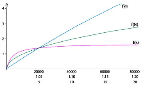
The Fundamental Resolution Equation indicates that resolution is affected by three important parameters: efficiency (N), selectivity () and retention factor (k) (Figure I-2). One can improve resolution by improving any one of these parameters. A value of 1 is the minimum for a measurable separation to occur and to allow adequate quantitation. Compared to gas chromatography (GC), HPLC is characterized by a relatively low resolving power which is mainly caused by the restricted length of the analytical columns.
Figure I-2. Resolution as a function of efficiency, selectivity and
retention factor.
Various approaches have been reported to establish an increase in LC resolving power and they will be discussed in the following chapters II and IV.
1.3. Detection
The chromatographic detector is able of determining both the identity and concentration of eluting components in the mobile phase stream. A wide range of detectors is available to meet different sample requirements, among which there are UV detectors, evaporative light scattering detectors (ELSD), mass
spectrometers (MS), refractive index (RI) detectors, fluorescence detectors, and electrochemical detectors. The most popular detectors in LC are UV-type, based on the solute adsorption of UV-VIS wavelengths, and MS, capable to measure with different accuracy the mass of a component. UV detectors can work either at a fixed wavelength, usually corresponding to the analyte maximum absorption (UV detectors), and at variable wavelength (photo diode array, PDA), making possible simultaneous monitoring of more than one absorbing component at different wavelengths. This detector extracts more information from the chromatogram and provides important data for the qualitative analyses of unknown samples, even if non-absorbing compounds cannot be detected at all. On the contrary, MS is an universal detector, specific enough to support the positive identification of a compound, offering structural information and/or the molecular weight (MS technique will be the subject of the chapter V). Beside, the ELSD is often used in HPLC; such detector enables the non-selective detection of non-volatile analytes. After removal of mobile phase by passing through a heated zone, the solute molecules are detected by light scattering depending on molecular sizes.
1.4. General trends
Since its advent, LC is being exploited by separation scientists and applied to a wider and wider range of sample matrices for the separation, identification and quantification of ever more compounds. The unceasing progresses in columns and stationary phases production, and the enormous developments in detection techniques, have contributed to the outstanding success of chromatography, as an invaluable tool in analytical chemistry, in many different fields including nutraceutical, food, environmental, clinical, forensic, and pharmaceutical applications. The great advantages to be gained by the use of LC are especially increased with the hyphenation to MS (LC-MS). Recent trends in the area of
LC-MS and related techniques involve: (i) the shift from conventional HPLC-MS to ultra high pressure liquid chromatography (UHPLC)-HPLC-MS or other fast LC-MS techniques (core-shell particles, high-temperature LC and monolithic columns), requiring fast MS analyzers (typically time-of-flight (ToF)-based systems); (ii) the use of supercritical fluid chromatography (SFC) for fast and “green” separations, with reduction in solvents consumption; (iii) the use of multidimensional liquid chromatography techniques (MDLC) for complex samples, and other dimension also in MS, such as ion mobility spectrometry (IMS)-MS and the coupling of two or more mass analyzers (tandem MS); (iv) the shift from low-resolution to (ultra)high-resolution MS to allow accurate mass measurements. Each of these techniques will be described in detail in the following chapters.
REFERENCES
- Horváth C., Lipsky S. R., Nature 1966, 211, 748-749.
- Howard G.A., Martin A. J. P., Biochem. J. 1950, 46, 532-538. - Martin A.J.P., Synge R.L.M., Biochem. J. 1941, 35, 1358-1368. - Saito Y., Jinno K., Greibrokk T., J. Sep. Sci 2004, 27,1379-1390.
Ultra High Pressure Liquid Chromatography
9 2.1. Introduction
Over recent decades, different advances in the development of comprehensive solutions to increase the separation efficiency and reduce the analysis time have been made. Different approaches have been reported to provide improved chromatographic separation. Among these, silica-based monolith columns, which consist of a single piece of porous material with several unique features in terms of high permeability and efficiency, plus low resistance to mass transfer, could be interesting (Luo, et al., 2005; Miyamoto, et al., 2008). However, the limited number of available columns dimensions and surface chemistries has restricted the progress of this technology. Another possible way to increase the efficiency on standard LC instrumentation consists in the use of long columns by coupling standard LC columns with totally porous particles and operation at high temperatures, allowed by the reduced mobile phase viscosity and hence lower pressure drop along the analytical column (Lestremau, et al., 2006; Plumb, et al., 2007; Sandra & Vanhoenacker, 2007). Unfortunately, the technical constraints as the longer analysis time, the limited number of available stationary phases capable of withstanding elevated temperatures, and the question of stability of the analytes, make this approach difficult to practice. Analogously, the use of partially porous stationary phases, also known as fused core or core-shell particles, allows to serially couple columns and boost the separation efficiency (Wang, et al., 2006; Cunliffe & Maloney, 2007; Cabooter, et al., 2008). The stationary phase particle consists of a thin layer of porous shell fused to a solid particle (Figure II-1). This technology drastically reduces the pressure drop when compared to fully porous (sub-2 μm) stationary phases, mainly when high temperatures are applied,
making it possible to operate such phases on a conventional LC instrument (Fekete, et al., 2014).
Figure II-1. Partially porous technology (Fused core, on the left) and totally
porous particles (on the right).
Since the introduction of the first commercially available HPLC columns packed with 10 μm particles in the early 1970s, the use of ever smaller particles has become the most popular way to improve chromatographic separations (Snyder, 2000; Gritti & Guiochon, 2012; Unger, et al., 2000; Eeltink, et al., 2004).
As reported by Giddings in 1991, there is a linear correlation between the pressure drop (ΔP) and the linear velocity (u) in the column (Giddings, 1991) (Equation II-1): p d uL P2 (Eq. II-1)
where ϕ, η, L, and d are the flow resistance, viscosity of the mobile phase, length of the column, and particles diameter, respectively. It has been
demonstrated that using a column 25 cm long packed with 5 μm particles an inlet pressure <25 bar is required for the chromatographic analysis, whereas reducing at 1 μm the particles diameter needs an inlet pressure of 2000 bar (Colon, et al., 2004; Anspach, et al., 2007). Consequently, dedicated instrumentation and columns are necessary (MacNair, et al., 1999; Shen, et al., 2005; Plumb, et al., 2006; de Villiers, et al., 2006a). Recent HPLC developments have been focusing, on the one hand, on the design of pumping devices, injection system and flow paths, capable of operating at very high pressures (600 to 1000 bar) and detectors capable of high acquisition rate; on the other hand, on the manufacturing of stationary phase particles that are stable enough to tolerate such elevated pressures. The term “ultra-high pressure liquid chromatography” (UHPLC) to describe the higher performance achieved by the novel instrumentation, in combination with small particles, was coined by Jorgensen in 1997 (MacNair, et al., 1997). Nowadays this technique is also known with the name of “ultra-high performance liquid chromatography” (UPLC). The first commercially available UHPLC system was introduced in 2004. The real success of any UHPLC system is correlated to the use of columns packed with sub-2 μm particles. The Van Deemter plot (Figure II-2) shows that smaller particles have the advantage of much flatter H values at higher flow velocities. This result means that speed can not only be doubled by halving particle diameter, but can also be doubled and doubled again by operating at higher flow velocities, without any efficiency loss. The numerous applications on UHPLC suggest a considerable enthusiasm towards this technique (Aguilera-Luiz, et al., 2008; Motilva, et al., 2013; Beltrán, et al., 2009; Wilson, et al., 2005; Cai, et al., 2009). Compared to conventional HPLC, it offers a series of advantages such as improved resolution, higher peak efficiency, shorter retention times, and reduced solvent consumption. Furthermore the narrower peaks (sharper peaks) and the lower detection limits
(LODs), due to the higher peak efficiency, provide for a greater sensitivity than HPLC. On the other hand, the technique is easily prone to several deficits. One of the major problems associated to the application of elevated pressures is the heating of the mobile phase due to viscous friction losses (Martin & Guiochon, 2005; de Villiers, et al., 2006b; Neue & Kele, 2007). This could produce radial or axial temperature gradients inside the column related to the thermal conditions under which the analysis is performed (isothermal or adiabatic operation, respectively). Both temperature gradients may compromise the separation efficiency.
Figure II-2. Van Deemter Plot at different dp.
2.2. UHPLC system requirements
The development of UHPLC systems represents an engineering challenge, since these instruments have to be designed to take advantage of the greater speed, higher resolution and superior sensitivity offered by small particles.
operation of UHPLC:
Instrument performance. It must be able to withstand the increased higher pressures than HPLC system, by improving the pressure capabilities of the pumping device.
Extra-column volume. The tubing volume, the mixer volume, the detector cell volume must be reduced as much as possible. A system plumbed with 0.005’’ I.D. stainless steel tubing and zero dead volume fittings is preferred for UHPLC experiments.
Dwell volume. It represents the volume of liquid contained in the system between the point where the gradient is formed and the point where the mobile phase enters the column. This volume includes the mixer, transfer lines, and any swept volume (including the sample loop) in the injection system. After the gradient has started, a delay is observed until the selected proportion of solvent reaches the column inlet, on account of this the sample is subjected to an unwanted additional isocratic migration. The dwell volume may differ from one instrument to another, but it can be easily measured (Dolan, 2006).
Mobile phases. It is recommended the use of high-grade organic solvents (recognized UPLC or LC-MS grade), Milli-Q water or similar, being careful to microbiological growth, and store the column with pure organic solvent, because of the size of the frits and particles that are much smaller than HPLC (0.2 μm versus 2 μm).
Column dimension. The separation is made faster by using shorter columns, but the same should still offer sufficient column efficiency to allow at least a baseline separation of analytes. If the primary goal is speed, it is recommended the use of a column with a length of 50 mm, otherwise it is preferable a column of 100 mm, if the main purpose is resolution. Reducing the column diameter does not shorten the analysis time, but decreases mobile
phase consumption and sample volume. It is possible to find UHPLC columns with 1.0, 2.1, 4.6 mm I.D. The 2.1 mm I.D. column should be considered as optimal, while 4.6 mm I.D. can generate significant frictional heating. Concerning the 1.0 mm I.D., the compatibility between the column geometry and any UHPLC instrument is critical, and it is only used for specific reasons (e.g. severely sample limited or direct flow to MS).
Detector acquisition rate. The narrow peaks generated in UHPLC have to be monitored by detectors that offer acquisition rates high enough to record a reasonable data points (20 points per peak are recommended) across the chromatographic peak. Only the latest generation of instruments meets these requirements.
2.3. Moving a HPLC method to an UHPLC
When transferring methods from HPLC to UHPLC, it is usually sufficient to maintain the resolution of the original method. A widespread approach consists in the employment of shorter columns packed with smaller particles; this strategy maintains resolution and allows faster separations. Several calculations are required to adapt some parameters, such as injection volume, flow rate, dwell volume, in both isocratic and gradient modes, to the new column characteristics.
2.3.1. Isocratic mode
In isocratic mode it is important to consider and thus adjust the flow rate and the injection volume. The linear velocity of the mobile phase has to be increased while decreasing the particle size to work within the Van Deemter optimum. In addition, the new flow rate is scaled to the change of column cross section if the column inner diameter changes. Specifically, it must be decreased as column internal diameter decreases. The UHPLC flow rate (F2) can be
calculated with the following equation: F2 =F1 ∙ ( 1 2 2 2 c c d d . 2 1 p p d d ) (Eq. II-2)
where dp is the particle size. Also the injection volume should be adapted to the
new column dimension, since it is proportional to the column volume. Indeed, decreasing the column internal diameter and length decreases the overall column volume and sample capacity. The new injection volume (VI2) can be
calculated with the Equation II-3:
VI2 = VI1 . 1 2 2 2 c c d d . 1 2 L L (Eq. II-3)
where dc and L represent the diameter and the length of the column,
respectively. Practically it is important to maintain the ratio of column dead volume and injection volume constant.
2.3.2. Gradient mode
Transferring an optimized gradient elution method between instruments, columns, etc. is more difficult than transferring isocratic elution method. Gradient methods can introduce variables that may not be easy to control. First of all, the same considerations about the flow rate and volume injection (Eq. II-2 and II-3) should be made. Either linear gradient or step gradient can be dissected into a combination of isocratic or gradient walks (Stoll, et al., 2006). For the isocratic step (tiso2) can be applied the following equation:
tiso2 = tiso1 . ( 1 2 c1 2 c2 2 2 1 L L . d d . F F ) (Eq. II-4)
this is useful also for the re-equilibration time. For the gradient step, the guidelines proposed by Schellinger and Carr should be followed (Schellinger & Carr, 2005). In order to maintain a constant selectivity, the start and the final composition of the mobile phase in the gradient should be the same than the original method: tgrad2 = 2 start1 final1 slope ) %B -(%B (Eq. II-5)
where slope2 is the slop of the new gradient and it is can be calculated with the
Equation II-6: slope2 = slope1 . ( 2 1 FF . 2c1 c2 2 d d . 1 2 LL ) (Eq. II-6)
even if this ploys is employed, the selectivity could be different because of different dwell volume (Guillarme, et al., 2012). In view of this, one must adjust the “effective” dwell volume, which is the total volume of starting eluent delivered to the column inlet after injecting the solutes. The “intrinsic” dwell volume is the gradient delay volume delivered to the column before the front of the gradient arrives at the column inlet. The latter is obviously an instrument constant, while the former is a modifiable parameter by delaying the injection or using an initial isocratic step (Schellinger & Carr, 2005).
REFERENCES
- Aguilera-Luiz M.M., J.L.M. Vidal, R. Romero-González, A. Garrido Frenich, J. Chromatogr. A 2008, 1205, 10-16.
- Anspach J.A., Maloney T.D., Colon L.A., J. Sep. Sci. 2007, 30, 1207-1213. - Beltrán E., Ibáñez M., Sancho J.V., Hernández F., Rapid Commun. Mass Spectrom. 2009, 23, 1801-1809.
- Cabooter D., Lestremau F., Lynen F., Sandra P., Desmet G., J. Chromatogr. A 2008, 1212, 23-34.
- Cai S.S., Syage J.A., Hanold K.A., Balogh M.P., Anal. Chem. 2009, 81, 2123-2128.
- Colon L.A., Cintron J.M., Anspach J.A., Fermier A.M., Swinney K.A., Analyst 2004, 129, 503-504.
- Cunliffe J.M., Maloney T.D., J. Sep. Sci. 2007, 30, 3104-3109.
- de Villiers A., Lestremau F., Szucs R., Gelebart S., David F., Sandra P., J. Chromatogr. A 2006, 1127, 60-69.
- de Villiers A., Lauer H., Szucs R., Goodall S., Sandra P., J. Chromatogr. A 2006, 1113, 84-91.
- Dolan J.W., LCGC North Am. 2006, 24, 458-466.
- Eeltink S., Decrop W.M.C., Rozing G.P., Schoenmakers P.J., Kok W.Th., J. Sep. Sci. 2004, 27, 1431-1440.
- Fekete S., Guillarme D., Dong M.W., LC GC N. Am. 2014, 32, 2-12. - Giddings J.C., Unified separation Science, Wiley, New York, 1991. - Gritti F., Guiochon G., J. Chromatogr. A 2012, 1228, 2-19.
- Guillarme D., Veuthey J.L., Smith R.M., Royal Society of Chemistry 2012. - Lestremau F., Cooper A., Szucs R., David F., Sandra P., J. Chromatogr. A 2006, 1109, 191-196.
- Luo Q.Z., Shen Y.F., Hixson K.K., Zhao R., Yang F., Moore R.J., Mottaz H. M., Smith R.D., Anal. Chem. 2005, 77, 5028-5035.
- MacNair J.E., Lewis K.C., Jorgenson J.W., Anal. Chem. 1997, 69, 983-989. - MacNair J.E., Patel K.D., Jorgenson J.W., Anal. Chem. 1999,71, 700-708. - Martin M., Guiochon G., J. Chromatogr. A 2005, 1090,16-38.
- Miyamoto K., Hara T., Kobayashi H., Morisaka H., Tokuda D., Horie K., Koduki K., Makino S., Nunez O., Yang C., Kawabe T., Ikegami T., Takubo H., Ishihama Y., Tanaka N., Anal. Chem. 2008, 80, 8741-8750.
- Motilva M.J., Serra A., Macià A., J. Chromatogr. A 2013, 1292, 66-82. - Neue U., Kele M., J. Chromatogr. A 2007, 1149, 236-244.
- Plumb R.S., Rainville P., Smith B.W., Johnson K. A., Castro-Perez J., Wilson I.D., Nicholson J.K., Anal. Chem. 2006, 78, 7278-7283.
- Plumb R.S., Mazzeo J.R., Grumbach E.S., Rainville P., Jones M., Wheat T., Neue U.D., Smith B., Johnson K.A., J. Sep. Sci. 2007,30, 1158-1166.
- Sandra P., Vanhoenacker G., J. Sep. Sci. 2007, 30, 241-244.
- Schellinger A.P., Carr, P.W., J. Chromatogr. A 2005, 1077, 110-119.
- Shen Y., Zhang R., Moore R.J., Kim J., Metz T.O., Hixon K.K., Zhao R., Livesay E.A., Udseth H.R., Smith R.D., Anal. Chem. 2005, 77, 3090-3100. - Snyder L.R., Anal. Chem. 2000, 72, 412-420.
- Stoll D.R., Paek C., Carr P.W., J. Chromatogr. A 2006, 1137, 153-162.
- Unger K.K., Kumar D., Grun M., Buchel G., Ludtke S., Adam T., Schumacher K., Renker S.J., Chromatogr. A 2000, 892, 47-55.
- Wang X., Barber W.E., Carr P.W., J. Chromatogr. A 2006, 1107, 139-151. - Wilson I.D., Nicholson J.K., Castro-Perez J., Granger J.H., Johnson K.A., Smith B.W., Plumb R.S., J. Proteom Res. 2005, 4, 591-598.
Supercritical Fluid Chromatography
19 3.1. Introduction
The use of supercritical fluids (SFs) for chromatography was first reported in 1962 by Klesper (Klesper, et al., 1962). In that study supercritical dichlorodifluoromethane and monochlorodifluoromethane were used as mobile phases to separate nickel etiporphyrin II from nickel mesoporphorin IX dimethyl ester. Since its introduction, SFC had a rapid rise as a new separation topic in the late 1980s and 1990s, before starting a slow decrease and almost waning for over a twenty-year span, in the shadow of other separation techniques. The last decade has been characterized by a renewed interest in this technique, as the introduction of a new generation of commercial instruments has given new stimulus to the development and application of SFC-based methodologies. SFC may be considered as a valuable alternative to conventional chromatographic techniques, and as such is being exploited by separation scientists and employed for a wide range of sample matrices. In the 1980s, SFC was mainly used with capillary columns and FID, while nowadays packed columns and LC type detectors are preferred, as this configuration is more robust and can be easily adapted to a broad range of analytes. Lee et al. (Lee & Markides, 1987) and Novotny (Novotny, 1989) were the first to introduce long capillaries or open tubular stationary phases for SFC in 1981, contributing in this way to the propagation of SFC among GC chromatographers. The latter were strongly attracted by the possibility to widen the power of GC techniques in terms of range of compounds that could be analyzed, while making only slight modifications to GC hardware to properly function with a supercritical fluid. Capillary SFC (cSFC) required pure CO2 as
temperature and pressure ramps were programmed to modify the elution strength in separations. Various passive devices were adopted for maintaining the critical pressure within the chromatographic instrument, from capillary tubing of small I.D. to integral frits; however, such homemade systems were often little rugged and suffered from poor reproducibility. Moreover, the properties of pure SF CO2 limited its use to only lipophilic compounds, and the
strong restrictions in terms of application caused the decline of cSFC in the 1990s. At the same time, a radical change of philosophy occurred based on works of Gere et al. (Gere, et al., 1982) and Berger (Berger & Deye, 1990a; Deye, et al., 1990; Berger & Deye 1990b). Enormous efforts were done for the development of SFC instruments dedicated to the use of LC-like packed columns (pSFC). The first commercial SFC system, based on LC equipment, was commercialized in 1983 by Hewlett Packard. The configuration included an innovative binary pump, offering the capability to modulate the properties of pure SF CO2 by directly modifying the mobile phase composition with the
addition of a modifier. Moreover, the backpressure could be maintained constant within the system, thanks to the presence of an active backpressure regulator (BPR), even under gradient elution. The technique was reported to provide better selectivity, shorter analysis times, and broader applicability also to polar compounds (Saito, 2013) than cSFC. However, the poor compatibility of pSFC with FID and the lower efficiency afforded by the use of short columns and 5 or 10 μm particles, beside the commercial success of LC characterized by superior repeatability and more rugged design of instrumentation, have contributed to the almost disappearance of SFC for nearly 20 years from analytical laboratories. Over the last decade, a renewed interest arouse within the chromatographic community, following the introduction of a new generation of instruments by a number of manufacturers (Waters, Agilent, Shimadzu). These pioneering systems are well suited to different analytical
purposes, and are capable to deliver efficiency and sensitivity rivaling with those offered by UHPLC. The novel BPR design, the higher upper pressure limits, and the reduced void volumes in fact make these instruments fully compatible with low diameter particles (<2 μm) and core-shell columns (Nováková, et al., 2014; Lesellier, 2012). On the other hand, preparative SFC (prep-SFC) has also proved to be a valuable tool for the isolation of sample constituents, or the purification of extracts (Pettinello, et al., 2000; Alkio, et al., 2000), strongly supported from the industry, to replace toxic and expensive normal phase solvents commonly employed at a preparative scale in HPLC.
3.2. Supercritical fluids and physico-chemical properties
Supercritical fluids were firstly defined by Cagniard de la Tour in his famous cannon barrel experiments in 1822 (Cagniard de la Tour, 1822), while the term “critical point” was coined by Andrews in 1869 (Andrews, 1869), as the end point of a liquid-vapor equilibrium curve, above which the heat of vaporization is null. This means that, above the critical point, there exists a state of matter that is continuously connected with both the liquid and the gaseous state: that is called a supercritical fluid. In SFC separation, the mobile phase consists of supercritical fluids, which are kept above their critical pressure and temperature; the nature of SFs vary markedly from that of liquid or gases, and the properties are considered to be a hybrid of these two physical states, which can be manipulated by changing some experimental parameters. The viscosity and diffusivity are similar to those of a gas, providing high solute diffusion coefficients (and limited pressure drop in the system) and faster separation kinetics (at increased flow rates without any loss in resolution). The density and solvating power of SFs are comparable to those of liquids, leading to good solubility and transportation of analytes; nevertheless SFs are more compressible than liquids, and that implies their density will severely change
with pressure and temperature. The latter will also affect the elution strength of the mobile phase, since the polarity of SFs directly increases with density. There are a number of possible fluids that may be used in SFC, but CO2 is by
far the most commonly used supercritical mobile phase nowadays, for various reasons. Ammonia, N2O, light hydrocarbons, water, and chlorofluorocarbons
cause serious problem related to toxicity, environmental pollution, and hardware corrosion, apart from being unsuitable for the analysis of thermolabile compounds (high critical temperature and critical pressure); instead, the use of CO2 has attracted particular attention because it is safe (low toxicity,
non-inflammable, non-corrosive), inert (no hardware damage), and easily available at high quality at a low price, (though it is abundant in the atmosphere, a large amount is also available as a by-product from NH3, H2 and ethanol production).
Moreover, CO2 offers good miscibility with both apolar (hexane, toluene, etc.)
and polar (water, alcohols, acetonitrile) organic solvents, and is also UV transparent down to 190 nm. Other advantages can be observed for preparative-scale separations in terms of recovery of concentrated fractions after separation (requiring less effort to evaporate solvents and thus recover pure fractions) and non-toxicity of residual amounts in human-contact products (Lesellier & West, 2015). But the real success of CO2 compared to other fluids consists in its low
critical point (31°C and 74 bar), as shown in Figure III-1, because these mild conditions are easily reached by conventional instrumentation and furthermore cause no degradation of the analytes (Taylor, 2010).
Figure III-1. Phase diagram of carbon dioxide (Nováková, et al., 2014).
CO2 is a highly nonpolar solvent, and its solvating power is considered similar
to that of hydrocarbons such as pentane or hexane. The non-polar character of SF CO2 favors the solubility of hydrophobic compounds, but limits the
application for the more polar analytes. In order to increase the elution strength of the mobile phase, small amounts (typically, 2-40%, v/v) of a polar solvent, called modifier or co-solvent, is usually added to SF CO2. Increased proportions
of modifier most often result in decreased retention, and peaks elute from lower to higher polarity. Most common used modifiers are isopropanol (IPA), methanol (MeOH), acetonitrile (ACN), ethanol (EtOH), and n-hexane; modifier addition will also improve peak shape and minimize peak tailing, either due to solubility improvement, or by masking some residual silanol groups on stationary phases of silica bonded with octadecyl groups and, thus, reducing the extent of unwanted interactions between the analytes and high energy sites. The modifier will change some physico-chemical properties of the mobile phase such as the viscosity and dielectric constant, and can generate further interactions such as hydrogen bonding or dipole-dipole, leading to modifications in selectivity. Therefore, the interactions with the stationary
phase may be too strong, and highly polar solutes may fail to elute, or elute with poor peak shapes. In order to overcome this drawback, a highly polar additive, such as a strong acid or base, is often dissolved in the modifier. The first use of additives to SFC eluent was reported in 1988 (Ashraf-Khorassani, et
al., 1988). The critical point of the mobile phase will considerably shift with
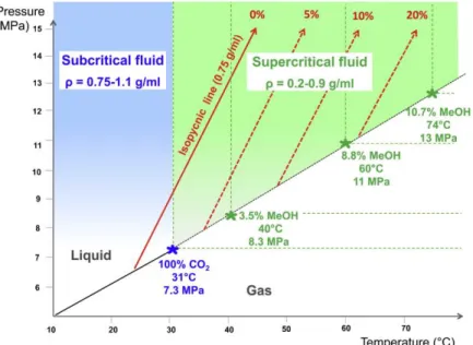
modifier addition: both the critical temperature and the critical pressure will increase, depending on the percentage and the nature of the modifier added to carbon dioxide, as shown in Figure III-2 (e.g. to reach 135°C and 168 bar for a 70:30 v/v CO2/MeOH mobile phase). This means that in most SFC separations,
the state of the mobile phase should be defined as “subcritical”, rather than “supercritical”, as with a working temperature typically not exceeding 60°C, whatever the gradient program, a subcritical fluid will be obtained very quickly upon increasing the proportion of modifier (Pinkston, et al., 2004). On the other hand, the increased elution strength produced by the presence of polar modifiers would be mostly connected to the proportion of the latter, rather than to the density modification associated with their presence; meantime the co-solvent will poorly influence the GC-like diffusivity and low viscosity.
Figure III-2. Phase diagram for pure carbon dioxide (in blue) or carbon
dioxide mixed with methanol at different proportions (in green).
The slanting red arrows indicate isopycnic lines (Lesellier & West, 2015).
3.3. Stationary phase types
Fused-silica capillary columns with cross-linked chemically bonded stationary phases, traditionally employed for high-resolution gas chromatography (HR-GC), have also been successfully exploited for SFC applications (King & List, 1996; King, 2003). Most of the recent work however is being described with packed HPLC columns. The absence of water in the mobile phase makes SFC a unified separation method because it allows the employment of both non-polar and polar stationary phases with the same mobile phase (Lesellier, 2009; Lesellier, 2008). SFC can replace RP-LC, non aqueous reversed phase liquid chromatography (NARP-LC), NP-LC, and hydrophilic interaction chromatography (HILIC), provided that the compounds of interest are soluble in the CO2. This means that practically all HPLC stationary phases are also
suitable to use in SFC, from octadecyl silica (ODS)-bonded silica to pure silica. However, they showed a number of inconveniences/limitations, the major being
poor selectivity and low sample capacity in SFC separations compared to the HPLC counterpart; moreover, the poor peak shape obtained for the separation of acidic or basic analytes required the use of additives in the mobile phase. More recently, new stationary phases especially designed for SFC have been developed, in the attempt to overcome such issues (Poole, 2012). The silica-based polymer-encapsulated has been probably the first type of stationary phase to find larger use in SFC than in HPLC, consisting of fully porous silica particles coated with a polysiloxane layer functionalized with polar groups or alkyl substituents. Such columns are not more in use nowadays, mainly because of problem associated to the free residual silanol activity, which was hampering the separation of more polar compounds. A number of novel SFC-specific stationary phases have been recently introduced to minimize such inconvenience, which include bonding and ligands designed and optimized for use in CO2-based separations. One of the most popular is a chemically bonded
phase with a 2-ethylpyridine substituent, affording decreased undesirable interactions among the silanol groups and the polar compounds, since the hydrogen-bonding between free silanol groups and the nitrogen atom of the pyridine ring, or partial protonation of the pyridine group (due to the acidity of carbon dioxide-methanol mobile phases) would repel positively charged analytes from the stationary phase, reducing interactions with the silanol groups. The use of such a phase decreases or eliminates the need for additives, and it is well suited to the analysis of a wide range of basic, as well as neutral and acidic compounds. The same mechanism of interaction (hydrogen-bonding or steric protection) can be encontered with silica-based support having amino, amide, urea and sulfonamide groups (Poole, 2012).
3.4. Instrumentation
A system for SFC can be easily developed starting from GC or LC equipment, on condition that facilities for temperature and pressure programming are available. In SFC separations it is very important to maintain the column outlet at a pressure above the critical one; in this regard a backpressure regulator is located after the column. This can be a simple capillary tube (passive backpressure regulator) or a device allowing the modification of this parameter (dynamic backpressure regulator). Most remarkably, some detectors must operate at elevated pressures, e.g. with UV detection pressure resistant cells are necessary (upto 400 bar). Commonly, SFC instruments consist of a binary pumping system: one pump is used to propel the CO2 and the other one is
dedicated to the organic modifier. The former is usually supplied from steel cylinders containing liquefied CO2 in contact with a gaseous headspace at 55 to
85 bar near room temperature, since reciprocating pumps cannot compress a low density gas because of a low compression ratios. Instead the modifier is a liquid at room temperature and pressure; separate pumps are hence required to avoid mismatches in pressure. It is necessary to cool the CO2 pump to below
4°C (generally, through an electronic cooling unit), to prevent any decrease in pressure or increase in temperature during the pump refill stroke; this would bring to vaporization of the liquid, and the pump would produce gaseous cavities in the liquid flow. Usually, a sample loop injection device is employed, and the column oven is nearly identical to that of an LC system. Finally, both GC type and LC type detectors can be coupled, the latter being more used nowadays. Specifically, in a GC-like SFC set-up, where only pure CO2 is used
as the mobile phase, FID, IR, electron capture detection (ECD), chemiluminescence, and various other detection approaches are possible, instead in a LC-like set-up, in the presence of a modifier, ELSD, UV, MS and, sometimes, charged aerosol detection (CAD) and acoustic flame detection
(AFD) are employed. Earlier implementations of SFC-MS followed the evolution of both HPLC-MS and GC-MS interfaces (Zaugg, et al., 1987; Arpino, et al., 1990; Crowther & Henion, 1985). The hyphenation of SFC to the mass analyzers is provided by means of electrospray ionization (ESI) or atmospheric pressure chemical ionization (APCI), much like in HPLC-MS (Lesellier & West, 2015).
3.4.1. Towards ultra high performance SFC
The ACN (the most widely used solvent in RP-LC) shortage of 2008 has had a direct negative impact on HPLC, in ways such as increases in the cost of solvent reprocessing, forcing chromatography users to consider solutions that consume less solvent. Based on these needs, important instrument manufacturers considered it vital to turn to greener technologies that have to be able to preserve high performance and productivity.
A number of improvements in the design of new systems have led to the introduction of the first instrument fully dedicated to high-performance analytical SFC, developed by Waters Corporation and commercialized with the name of Ultra-Performance Convergence Chromatography (UPC²). Compared to old generation SFC instruments, with this technology, the reliability and precision of pumping system and backpressure regulation, required for controlling the delivery of mixtures of CO2 and organic modifier over a broad
range of flow rates and pressures, were drastically enhanced. A two-stage back pressure regulator (BPR) (passive + active) was assembled on the UPC2 instrument, in which the passive component maintains pressure at 104 bar, while the active component provides for further backpressure increase and fine adjustments. This device ensures repeatable mobile phase density conditions and retention times between successive analyses, adapting itself fairly quickly to modifications in mobile phase composition or flow.
The new instrument design also includes reductions in injection volume and detector-cell volume, and minimized connector tubing length and diameter. All these improvements offer increases in throughput and in the efficiency of the analyses, especially when used in combination with sub 2-µm particles at the limit pressure tolerate by the system. In this regard, it must be pointed out that this system allow for a maximum pressure of 400 bar. Despite its lower inlet pressure limit, the optimum linear velocity is higher by a factor of 3-5-fold than in UHPLC, allowing ultra-fast and/or highly efficient analysis (Grand-Guillaume Perrenoud, et al., 2012b). This justifies introduction of the term ultra high performance SFC (UHPSFC) as an appellation for the combination of state-of-the-art SFC set-up and columns packed with sub-2 μm particles (Grand-Guillaume Perrenoud, et al., 2012a). A schematic of UPC2 instrumentation is illustrated in Figure III-3.
REFERENCES
- Alkio M., Gonzalez C., Jännti M., Aaltonen O., JAOCS 2000, 77, 315-321. - Andrews T., Philosophical Transactions of the Royal Society (London) 1869, 159, 575-590.
- Arpino P.J., Dilettato D., Nguyen K., Bruchet, A., J. High Res. Chromatog. 1990, 13, 5-12.
- Ashraf-Khorassani M., Fessahaie M.G., Taylor L.T., Berger T.A., Deye J. F., J. High Res. Chromatog. 1988, 11, 352-353.
- Berger T.A., Deye J.F., Anal. Chem. 1990, 62, 1181-1185. - Berger T.A., Deye J.F., Chromatographia 1990, 30, 57-60.
- Cagniard de la Tour C., Annales de chimieet de physique 1822, 21, 127-132. - Crowther J.B., Henion J.D., Anal. Chem. 1985, 57, 2711-2716.
- Deye J.F., Berger T.A., Anderson A.G., Anal. Chem. 1990, 62,615-622. - Gere D.R., Board R., McManigill D., Anal. Chem. 1982, 54, 736-740.
- Grand-Guillaume Perrenoud A., Boccard J., Veuthey J.-L., Guillarme D., J. Chromatogr. A 2012, 1262, 205-213.
- Grand-Guillaume Perrenoud A., Veuthey J.-L., Guillarme D., J. Chromatogr. A 2012, 1266, 158-167.
- King J.W., List G.R., AOCS Press, Champaign 1996.
- King J.W., (R. O. Adlof, ed.) Oily Press, Bridgewater 2003, 301-366. - Klesper K., Corwin A.H., Turner D.A., J. Org. Chem. 1962, 27, 700-706. - Lee M.L., Markides K.E., Science 1987, 235, 1342-1347.
- Lesellier E., J. Chromatogr. A 2009, 1216, 1881-1890. - Lesellier E., J. Chromatogr. A 2012, 1228, 89-98. - Lesellier E., J. Sep. Sci. 2008, 31, 1238-1251.
- Lesellier E., West C., J. Chromatogr. A 2015, 1386, 2-46.
- Nováková L., Perrenoud A.G-G., François I., West C., Lesellier E., Guillarme D., Anal.Chim. Acta 2014, 824, 18-35.
- Novotny M.V., Science 1989, 246, 51-57.
- Pettinello G., Bertucco A., Pallado P., Stassi A., J. Supercrit. Fluids 2000, 19, 51-60.
- Pinkston J.D., Stanton D.T., Wen D., J. Sep. Sci. 2004, 27, 115-123. - Poole C.F., J. Chromatogr. A 2012, 1250, 157-171.
- Saito M., J. Biosci. Bioeng. 2013, 115, 590-599. - Taylor L.T., Anal. Chem. 2010, 82, 4925-4935.
- Zaugg S.D., Deluca S.J., Holzer G.U., Voorhees K.J., J. High Res. Chromatog. 1987, 10, 100-101.
Multidimensional Liquid Chromatography
33 4.1. Introduction
There are a whole host of real mixtures that are profitable to separate for qualitative and quantitative analysis, but simply can not be due to their complex nature. Obviously, these mixtures can be separated to some extent by using one-dimensional chromatography (1D-LC), but even in optimum conditions and with the most efficient column, full separation from single column chromatography will never be achieved. Moreover, even in samples of low complexity there is generally a random peak distribution, which requires high plate number values for total peak resolution (Guichon, 2006; Davis, et al., 1983). In particular, if the number of components exceeds 37% of the peak capacity, peak resolution is statistically compromised (Davis, et al., 1983). The limited resolving power of 1D-LC has incited the development of multidimensional LC (MDLC), in which the sample is subjected to two different separation mechanisms. The largest benefit of pairing columns, with different selectivity in a MDLC configuration, is the dramatic increase of the peak capacity, which is reflected in the reduction of component overlap. The first recorded use of two-dimensional chromatography was reported by Consden et al. (Consden, et al., 1947), who separated 22 hydrochlorides of amino acids by using paper chromatography. Combinations of chromatography ×electrophoresis (Haugaard & Kroner, 1948) and electrophoresis×electrophoresis (Durrum, et al., 1951) were also made early in the life of multidimensional separations. Two-dimensional thin-layer chromatography (2D-TLC) was pioneered by Kirchner et al. (Kirchner, et al., 1951) and quickly became a popular technique. Following, great efforts were made to develop two-dimensional gas chromatography (2D-GC) (Deans, 1968;
Deans, 1971). In 1978 Enri and Frei (Erni & Frei, 1978) described the usage of off-line and on-line approaches to two-dimensional liquid chromatography (2D-LC). However, the first truly comprehensive 2D-LC work did not occur until 1990, when Bushey and Jorgenson performed the separation of a protein sample with a microbore cation-exchange column in the first dimension (1D) and a exclusion column in the second dimension (2D) (Bushey & Jorgenson, 1990). This publication has experienced large interest in the technique in different fields, and in recent years, because of commercially available systems, has been the subject of various reviews (Liu & Lee, 2000; Evans & Jorgenson, 2004; Shellie & Haddad, 2006; Jandera, 2006; Tranchida, et al., 2007; Dugo, et al., 2008a; Dugo, et al., 2008c).
4.2. Multidimensional chromatography approaches
Several approaches may be used when coupling different separation mechanisms in 2D-LC, namely off-line, on-line, and stop-flow (also known as stop-and-go) methods, which can be distinguished on the basis of the transfer mode from the 1D to the 2D.
In off-line approach, fractions from the first dimension column are collected (manually or via a fraction collector) and stored indefinitely after concentration by partial or complete evaporation (if necessary), and finally injected onto the second dimension column. In off-line mode, only a single liquid chromatograph is sufficient to perform a 2D-LC separation and only a little attention is required regarding the compatibility of the mobile phases (immiscible solvents can be evaporated after which the sample components are re-dissolved in the appropriate second dimension injection solvent). Furthermore, there is no time constraint for either dimension and therefore, practically no high limit to the separation power available. The main drawbacks are the possibility of sample contamination, degradation or loss during handling (making this approach
almost useless for quantitative trace analyses), lack of automation (often causing poor reproducibility), its time consuming and operative intensive character.
In on-line coupling, fractions from the first dimension are sequentially transferred to the second dimension through an appropriate interface, typically a high-pressure switching valve. This approach is characterized by a high reproducibility, since the whole process is completely automated, and high sample throughput, but a number of technical requirements need to be fulfilled, in order to avoid mismatches arising from mobile phase miscibility employed in the two dimensions and the compatibility between the 1D mobile phase with 2D stationary phase. On-line method requires that analysis in the second dimension be completed before transfer of the following fraction. This constrains the separation in the second dimension to be concluded in what is usually a very short amount of time (generally, on the order of several seconds to one or two minutes). The 2D analysis time should be at least equal or less than the duration of a modulation period; this can often result in a limited separation power in the second dimension. To overcome such an issue, it is possible to speed up the separation in 2D by using a very high flow rate or a short column. In fact, the
enhancements in LC column technologies (fused-core or sub-2 μm particles) and instrumentation (UHPLC instruments able to work at pressure of 1000 bar and higher) allow to carry out very fast analysis in 2D with acceptable efficiency. Alternatively, the stop-flow strategy can be adopted. This set-up involves direct transfer of each fraction to the second dimension column, followed by stopping the flow in the first dimension whereas operating the separation in the second dimension, and replaying this process throughout the entire first dimension separation. This approach attenuates the time constraints of the second-dimension, but can result in overly long “peak parking” times,
which decreases the efficiency of the first-dimension separation (Gritti & Guiochon, 2006; Miyabe, et al., 2007).
Evidently, the high complexity of on-line system, the need for specific interfaces and software, the expertise degree of the analysts and also economic implications, make this technique less easy to use with respect to the off-line approach that can be easily accomplished, since both analytical dimensions can be optimized as two independent methods.
Both off-line and on-line 2D-LC can be distinguished on heart-cutting (LC-LC) and comprehensive (LC×LC) techniques (Schoenmakers, et al., 2003). The principal difference between the two approaches is the number of fractions that are transferred from the primary column effluent. In heart-cutting 2D-LC, only significant parts of the effluent, containing the compounds of interest, are transferred to the second dimension, permitting the rest of the first column effluent to exit the system through the waste, while comprehensive LC allows the separation of the complete (comprehensive) sample by the two dimensions. As stated, all these techniques are associated with a number of advantages and disadvantages, and normally the choice of configuration depends on the one hand by the purpose or problem of the separation, and on the other hand by the availability of instrumentation.
4.3. Theoretical concepts: peak capacity, orthogonality and sampling rate
The basic metric that represents the separation capability is the peak capacity (nc) which is defined as the maximum number of peaks that can fit side by side
between the first (or unretained) and last peak of interest, at a fixed resolution between all these peaks. For one-dimensional gradient separation, the peak capacity can be calculated using the well-known method defined by Neue (Neue, 2005):
n n g c n t n 1 / 1 1 (Eq. IV-1)where tg is the gradient time, ω is the baseline peak width, and n represents the
number of peaks selected for the calculation.
In a fully orthogonal 2D system, ideally the total peak capacity (nc,2D) is equal
to the product of the peak capacities in the first (1nc) and in the second (2nc)
dimensions: c c D c n n n,2 1 2 (Eq. IV-2)
However, the real increase in peak capacity is usually lower than predicted from Equation IV-2, depending on the degree of similarity of the coupled columns, as this value includes a region where there is retention correlation between the dimensions. In the calculation of the “practical peak capacity” (n’c,2D) interrelated factors, including orthogonality and sampling rate, must be
taken into consideration. Methods for calculating a truer nc,2D were proposed
and reviewed by Dixon and Perrett (Dixon & Perrett, 2006). The maximum gain in resolving power is achieved in so-called “orthogonal” systems, in which the minimum correlation between the two retention mechanisms must occur. This means that the two used separation principles have to be independent of each other and show distinct retention profiles. Practically, truly orthogonal systems are hard to achieve, as orthogonality not only depends on the separation mechanisms, but also on the properties of the analytes and the separation conditions. The best orthogonal combinations can be attained when the appropriate stationary and mobile phases are carefully selected with respect to the physico-chemical properties of the sample constituents like molecular
size, charge, acid-base nature, polarity, hydrophobicity, etc. A number of various stationary phases is nowadays available, with different characteristics regarding surface chemistries, support material, pore size, and carbon load, while mobile phase composition can be modified by adding ion pair agents or changing the modifier, pH, temperature. Some example of orthogonal combinations are: NP-LC×RP-LC, in which the separation occurs respectively on the basis of polarity and hydrophobicity (Dugo, et al., 2004), silver-ion (SI) LC×NARP-LC, which provides separation according to degree of saturation and hydrophobicity (Mondello, et al., 2005), and also the coupling of two RP-LC dimensions can give high orthogonality, despite the degree of correlation between similar or even identical stationary phases that may be reduced by adequately tuning analytes interactions; this can be accomplished through the use of different mobile phase pH values (Dugo, et al., 2013; Donato, et al., 2011) or by varying the gradient composition between subsequent 2D runs, according to the properties of the analytes being transferred from 1D (Leme, et
al., 2014). On the other hand, retention in orthogonal combination could be
slightly related because of similar physico-chemical properties of some molecule in the sample. For example, size exclusion chromatography (SEC)×RP-LC or SEC×NP-LC may exhibit some selectivity correlation as the high contribution of hydrophobic or polar interactions in large molecules; in the same way ion-exchange (IEX) LC separates analytes mainly on the basis of charge, but might show hydrophobic or polar interactions.
The concept and meaning of orthogonality are better illustrated in Figure IV-1 and are clarified by practical examples of RP-LC×RP-LC (on the right: not orthogonal set-up due to the same retention mechanisms and same pH mobile phases) and HILIC×RP-LC (on the left: orthogonal set-up due to two independent retention mechanisms).
Evidently, low orthogonality is observed when the blobs obtained by plotting the retention times of the two dimensions are spread in the two-dimensional space mostly along a line, usually over a diagonal of the contour plot, instead of a random peak distribution able to completely cover the 2D map. Consequently, the determination of orthogonality is essential in order to evaluate the efficiency of the technique in terms of peak capacity and maximize the separation space available for the separation of complex samples. Various approaches have been studied for the calculation of the 2D system orthogonality, among which: the spreading angle method of Liu et al. (Liu, et al., 1995), the informational theory of Slonecker et al. (Slonecker, et al., 1996; Gray, et al., 2002), and a more recent approach proposed by Camenzuli and Schoenmakers (Camenzuli & Schoenmakers, 2014).
Figure IV-1. Representation of orthogonality in comprehensive LC