Dipartimento di Science Biologiche, Geologiche e
Ambientali
Corso di Dottorato di Ricerca in Scienze Geologiche, Biologiche e
Ambientali - XXX Ciclo
Innovative numerical petrological methods for
definition of metamorphic timescale events of
southern European Variscan relicts via
thermodynamic and diffusion modelling of zoned
garnets
Tesi di Dottorato di Ricerca di
Roberto Visalli
Tutor
Coordinatore
Prof. Rosolino Cirrincione
Prof.ssa Agata di Stefano
Co-Tutor
Prof. Gaetano Ortolano
List of Contents
ABSTRACT ... 12
RIASSUNTO ... 13
1. INTRODUCTION ... 17
1.1 Aims ... 24
2. “PETROMATICS” AND NUMERICAL PETROLOGY SUPPORTED BY IMAGE ANALYSIS ... 26
2.1 General outlines ... 26
2.2 Grain Size Detection (GSD): a new ArcGIS® toolbox to construct grain size distribution by drawing mineral grain boundaries on thin section scans ... 28
2.2.1 Pre-edge detection filter phase ... 31
2.2.2 Edge detector ... 33
2.2.3 Grain polygons creator ... 36
2.2.4 Final remarks ... 38
2.3 Quantitative X-ray Map Analyser (Q-XRMA): A new GIS-based statistical approach for Mineral Image Analysis... 38
2.3.1 Algorithms ... 41
2.3.1.1 First cycle: pre-calibration procedure ... 45
2.3.1.2 Second cycle: calibration algorithm ... 47
2.3.1.3 Second cycle: maps calibration (data setting and outputs) ... 52
2.3.1.4 Third cycle: mineral end-member maps ... 56
2.3.2 Case study ... 58
2.3.2.1 Garnet ... 59
2.3.2.2 Plagioclase ... 60
2.3.2.3 Biotite ... 62
2.3.3 Final Remarks ... 63
2.4 Mineral Grain Size Distribution (Min-GSD): a useful tool to display the grain size frequency distribution of each rock-forming mineral ... 64
3. THE DIFFUSION MODELLING TOOL APPLIED FOR DISCOVERING TIMESCALES AND RATES OF GEOLOGICAL PROCESSES ... 70
3.1 General Outlines ... 70
3.2 Diffusion mechanisms ... 74
3.3 Element diffusion coefficients ... 76
3.3.1 Factors affecting diffusion coefficient measurements ... 79
3.3.2 Diffusion coefficient map creator (DCMC): A Q-XRMAn image-processing add-on for creating map of various kinetic coefficients in a Local Information System (LIS) ... 81
3.4 Mathematics of diffusion ... 87
3.4.1 Basics of diffusion laws ... 87
3.4.2 Solutions of diffusion equations ... 91
3.4.2.1 Initial condition ... 92
3.4.2.2 Boundary conditions ... 93
3.4.2.3 Numerical solution: The finite-difference explicit method ... 96
4. CASE STUDIES ... 99
4.1 General outlines ... 99
4.2 First case study: Timescale of Late-Variscan static event constrained by garnet multicomponent diffusion modelling: new insights from the Serre Massif (Southern Calabria, Italy) 103 4.2.1 Introduction... 103
4.2.2 Geopetrological background ... 107
4.2.3 Methodology ... 110
4.2.4 Petrography and mineral chemistry ... 111
4.2.5 Image-assisted thermodynamic modelling ... 115
4.2.5.1 Quantitative image processing ... 117
4.2.5.2 Thermobaric constraints ... 122
4.2.6 Diffusion modelling ... 128
4.2.6.1 Image-assisted diffusion modelling ... 129
4.2.6.2 Sources of uncertain ... 136
4.2.7 Final Remarks ... 137
4.3 Second case study: Timescale and cooling of the Calabria continental lower crust inferred via garnet diffusion modelling: An example from the Sila Piccola Massif ... 139
4.3.1 Introduction... 140
4.3.2 Geological Background ... 141
4.3.3 Mesostructural features ... 143
4.3.4 Petrography and mineral chemistry ... 146
4.3.4.1 Methods ... 146
4.3.4.2 Petrographic description ... 146
4.3.4.3 Garnet-biotite-sillimanite paragneiss – CEL1B sample ... 149
4.3.5 Image-assisted thermodynamic modelling ... 151
4.3.5.1 Quantitative image processing and thermobaric constraints ... 152
4.3.6 Diffusion modelling ... 154 4.3.7 Final remarks ... 156 5. CONCLUSIONS ... 161 ACKNOWLEDGEMENTS ... 166 BIBLIOGRAPHY ... 168 APPENDICES ... 187
APPENDIX A1 – Grain size detection of thin sections ... 187
APPENDIX B2 – EMP analyses of the investigated phases ... 220
APPENDIX B3 – X-ray maps of the studied example domain ... 235
APPENDIX B4 – Input control spot analysis ... 236
APPENDIX B5 – Summary report of the multilinear regressions ... 246
APPENDIX B6 – EMP/Q-XRMA comparisons ... 269
APPENDIX C1 – EMP analyses of Serre Massif rocks ... 275
APPENDIX C2 – X-ray maps of garnet microdomains from Serre Massif rocks ... 301
APPENDIX C3 – XRF composition ... 302
APPENDIX C4 – Sample locations ... 302
APPENDIX C5 – Isopleth intersections ... 303
APPENDIX C6 – X-ray maps of a zoom in a garnet rim ... 304
APPENDIX C7 – Sequence of calculation adopted in the MATLAB scripts ... 304
List of Figures
Fig. 1.1 - Schematization of the sequential steps adopted to achieve the aims of the PhD project ... 25
Fig. 2.1 - Effect of the pre-processing phase on the input thin section scan. ... 29
Fig. 2.2 - Screenshot of the routine composing the Grain Size Detection toolbox ... 30
Fig. 2.3 - Flow chart of the Pre-edge detection filter phase routine ... 31
Fig. 2.4 - Schematic representation of the low filter principle used in the procedure... 31
Fig. 2.5 - Schematization of the single steps of the Pre-edge detection routine ... 32
Fig. 2.6 - Schematic representation of the high filter principle used in the procedure ... 33
Fig. 2.7 - Flow chart of the Edge detector filter phase routine ... 34
Fig. 2.8 - Schematization of the single steps of the Edge detector routine ... 35
Fig. 2.9 - Flow chart of the Grain polygons creator routine ... 36
Fig. 2.10 - Schematization of the single steps of the Grain polygons creator routine. ... 36
Fig. 2.11 - Difference between a smoothed vs. a non-smoothed polyline feature. ... 37
Fig. 2.12 - Effect of a non-completed boundary regarding the creation of polygon features ... 37
Fig. 2.13 - Simplified flow charts of the GIS-based image-processing procedure ... 41
Fig. 2.14 - Flow chart of the first cycle of the geoprocessing procedure ... 43
Fig. 2.15 - Flow chart of the second cycle of the geoprocessing procedure ... 44
Fig. 2.16 - Flow chart of the third cycle of the geoprocessing procedure ... 45
Fig. 2.17 - Example of schematic 3D representation of the decorrelation function ... 46
Fig. 2.18 - Example of possible relationship between dependent and explanatory variables ... 49
Fig. 2.19 - Difference between heteroscedasticity vs. Homoscedasticity distribution of the residuals. ... 51
Fig. 2.20 - Effect of outliers on the regression results (i.e., 𝑅𝑅2 values). ... 52
Fig. 2.21 - Point coordinates conversion spreadsheets ... 54
Fig. 2.22 - PtAnls.xlsx file used by the Python code to create an ArcGIS® point shapefile ... 55
Fig. 2.23 - Editing step of the ArcGIS® shapefile for removing points close to the edge mineral zones ... 55
Fig. 2.24 - Summary results of the calibration procedure using iron as a dependent variable ... 56
Fig. 2.25 - Window shell of the third analytical cycle ... 57
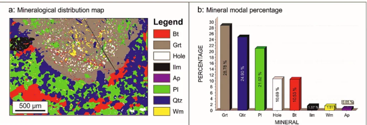
Fig. 2.26 - Output of the first analytical cycle ... 58
Fig. 2.27 - Outputs of the second and third analytical cycles for garnet... 59
Fig. 2.28 - Outputs of the second and third analytical cycles for plagioclase ... 61
Fig. 2.29 - Outputs of the second and third analytical cycles for biotite ... 62
Fig. 2.30 - Grain size distribution derivation ... 65
Fig. 2.31 - Thin Section X-ray map array. ... 66
Fig. 2.32 - Mineral classification of the entire thin section via Q-XRMA ... 67
Fig. 2.33 - Flow chart of the Mineral Grain Size Distribution toolbox ... 67
Fig. 2.34 - Grain size distribution distinct for each thin section-forming mineral ... 68
Fig. 3.1 - Schematic example of how diffusion works in a liquid ... 70
Fig. 3.2 - Schematization of particle diffusion between two solids in contact along their faces ... 71
Fig. 3.3 - Schematic representation of the proceeding of diffusion ... 73
Fig. 3.4 - Schematic representation of the main crystal lattice defects ... 75
Fig. 3.5 - Schematization of the various intergranular diffusion mechanisms ... 75
Fig. 3.6 - Different crystallographic structures influencing diffusion ... 80
Fig. 3.7 - Windows shell of the DCMC add-on showing the initial prompts ... 82
Fig. 3.8 - Windows shell of the DCMC tool showing the sequential operative step. ... 83
Fig. 3.9 - Flow chart of the DCMC geoprocessing procedure ... 84
Fig. 3.10 - Input data of the DCMC add-on ... 85
Fig. 3.11 - Temperature and Pressure maps derived by the DCMC. ... 85
Fig. 3.12 - Windows shell of the three-different diffusion coefficient calculations. ... 85
Fig. 3.13 - Mineral component concentration maps from the third analytical cycle of the Q-XRMA ... 86
Fig. 3.14 - Matrix of diffusion coefficients computed for garnet ... 86
Fig. 3.16 - Nomenclature for the mass balance of fluxes in a rectangular solid ... 89
Fig. 3.17 - Different cases of pre-diffusion initial condition ... 93
Fig. 3.18 - The diffusion process graphically illustrated for a half grain of a single phase ... 94
Fig. 3.19 - Visualization of the discretization of time and space used in finite difference algorithms ... 96
Fig. 3.20 - Example of a loop structure built in a MATLAB® script ... 98
Fig. 4.1 - Distribution of the Alpine and Pre-Alpine Basement in Western Europe. ... 99
Fig. 4.2 - Sketch of the possible configuration of Variscan Western Europe in Late Carboniferous ... 100
Fig. 4.3 - Geological map representations of the Calabria-Peloritani Orogen). ... 102
Fig. 4.4 - Geological framework of the Serre Massif ... 107
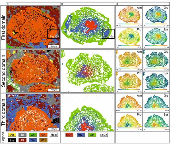
Fig. 4.5 - Garnet porphyroblasts showing different steps of the metamorphic evolution ... 113
Fig. 4.6 - Mineral chemistry of the samples investigated ... 114
Fig. 4.7 - Thin section classification ... 117
Fig. 4.8 - Three-selected investigated domains via Q-XRMA image processing procedure ... 121
Fig. 4.9 - Pseudosections computation supported by image analysis ... 123
Fig. 4.10 - New image-assisted 𝑃𝑃𝑃𝑃-path of the Serre Massif ... 127
Fig. 4.11 - Mineral grain size distribution of the MA271 sample ... 130
Fig. 4.12 - Schematic image-processing sequence to derive diffusion coefficient maps via DCMC ... 131
Fig. 4.13 - Diffusion modelling results obtained by using image-assisted thermodynamic modelling .... 133
Fig. 4.14 - Diffusion modelling results ... 135
Fig. 4.15 - Temperature-time diagram of the Upper Crust (Serre Massif) ... 138
Fig. 4.16 - Geo-structural map of the crystalline basement of the Sila Piccola ... 144
Fig. 4.17 - Mesostructural features in orthogneiss and metapelites of the Castagna Unit rocks ... 145
Fig. 4.18 - Observed microstructures representing two opposite sense of shear ... 148
Fig. 4.19 - CEL1B sample features ... 150
Fig. 4.20 - X-ray maps of the selected garnet domain from the CEL1B metapelite sample ... 151
Fig. 4.21 - Definition of the effective reactant volume (ERV) by image analysis ... 153
Fig. 4.22 - 𝑃𝑃𝑃𝑃 pseudosection of the syn-mylonitic assemblage for the CEL1B sample. ... 154
Fig. 4.23 - Diffusion model of the garnet retrograde zoning ... 156
List of Tables
Tab. 1.1 – Summary of the tools developed.………21Tab. 2.1 – Output of the 1st cycle for the selected domain in the Q-XRMA….……….58
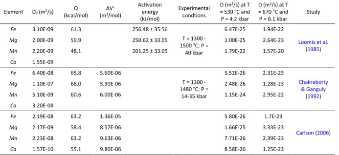
Tab. 3.1 – Datasets of diffusion data reported in the literature………81
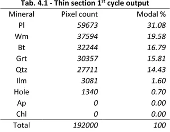
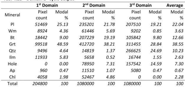
Tab. 4.1 – Thin section 1st cycle output for the first case study…...……….119
Tab. 4.2a – Domain 1st cycle output for the first case study…..………120
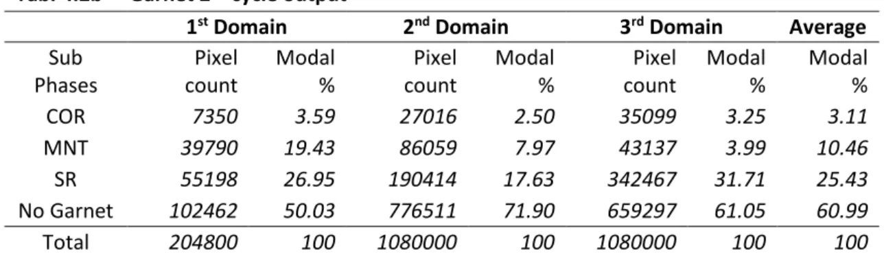
Tab. 4.2b – Garnet 2nd cycle output for the first case study………121
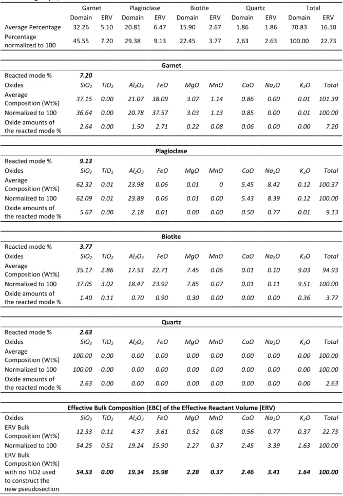
Tab. 4.3 – Calculation of oxide amounts to be fractionated from garnet porphyroblasts….……….126
Tab. 4.4 – Calculation of the effective bulk composition from the effective reactant volume….………127
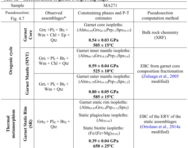
Tab. 4.5 – Reconstruction of garnet overgrowing stages……….128
Tab. 4.6 – Summary of diffusion coefficient expressed as a function of T and P…..……….134
List of Equations
Eq. 1 Generic diffusion equation when 𝐷𝐷 is constant
Eq.2 Interdependent multilinear regression algorithm
Eq. 3 Conversion of the analytical device 𝑋𝑋-coordinate when 𝑋𝑋 > 0 Eq. 3b Conversion of the analytical device 𝑋𝑋-coordinate when 𝑋𝑋 < 0 Eq. 3c Conversion of the analytical device 𝑌𝑌-coordinate when 𝑌𝑌 > 0 Eq. 3d Conversion of the analytical device 𝑌𝑌-coordinate when 𝑌𝑌 < 0
Eq. 4 Calculation of the interdiffusion coefficient
Eq. 5 Matrix of diffusion coefficients
Eq. 6 Calculation of the element of the diffusion matrix
Eq. 7 Effective binary diffusion coefficient calculation
Eq. 8 Calculation of diffusion coefficient as a function of 𝑃𝑃 and 𝑃𝑃
Eq. 9 Fick’s first law of diffusion
Eq. 10 Expression of the diffusion tensor for anisotropic medium
Eq. 11 Diffusion equation in presence of crystal growth/dissolution
Eq. 12a One-dimension fluxes in a 𝑛𝑛-multicomponent system
Eq. 12b Fick’s first law for a 𝑛𝑛-multicomponent system
Eq. 13a One-dimensional flux within a small solid volume
Eq. 13b One-dimensional compositional changes in a small solid volume
Eq. 13c Continuity equation
Eq. 14 Limit of the continuity equation
Eq. 15 Fick’s second law of diffusion
Eq. 16a Fick’s second law of diffusion when 𝐷𝐷 is constant
Eq. 16b Fick’s second law of diffusion when 𝐷𝐷 is not constant
Eq. 17 Compositional change along the spatial coordinate
Eq. 18a Forward difference scheme for the spatial coordinate
Eq. 18b Compositional change along the time coordinate
Eq. 19 Forward difference method when 𝐷𝐷 is constant
Eq. 20 Forward difference method when 𝐷𝐷 is not constant
List of Symbols
⟦ ⟧ Discretized positive value of a map’s pixel
⟦𝐶𝐶𝑖𝑖⟧ The absolute and discretized concentration of the element 𝑖𝑖
computed for each pixel
⟦𝐺𝐺𝐺𝐺𝑖𝑖⟧0255 The discrete pixel-intensity values of the 𝑖𝑖, 𝑗𝑗, 𝑘𝑘 … 𝑛𝑛, one-channel
elemental maps
𝛼𝛼1; 2; 3; …𝑛𝑛 Regression coefficients between the measured concentration
value of the elements and the corresponding pixel intensity value of the original X-ray raster images at the same point
𝛽𝛽𝑖𝑖 Value of the intercept for the element 𝑖𝑖
𝐶𝐶 Generic chemical concentration
𝐶𝐶𝑖𝑖, 𝐶𝐶1 Concentration of the component 𝑖𝑖
𝑪𝑪 A column vector of the concentrations of 𝑛𝑛 − 1 independent
components in an 𝑛𝑛-component system
𝐷𝐷 Generic diffusion coefficient
𝐷𝐷0 Pre-exponential factor (i.e., the self- or tracer coefficient)
𝐷𝐷𝑖𝑖, 𝐷𝐷1 Diffusion coefficient of an element 𝑖𝑖
𝐷𝐷𝑖𝑖−𝑗𝑗 Interdiffusion coefficient
𝑫𝑫 Matrix of diffusion coefficients
𝐷𝐷𝑖𝑖𝑗𝑗, 𝐷𝐷11 Element of the 𝑫𝑫-matrix
𝐷𝐷(𝐸𝐸𝐸𝐸) Effective binary diffusion coefficient
𝐷𝐷(𝑃𝑃, 𝑃𝑃) Diffusion coefficient expressed as a function of temperature and pressure
∆𝐺𝐺 Activation volume of diffusion
𝛿𝛿𝑖𝑖𝑗𝑗 Kronecker delta
𝑓𝑓𝑓𝑓2 Oxygen fugacity
𝐽𝐽𝑖𝑖, 𝐽𝐽1 Flux of a component 𝑖𝑖
𝐽𝐽𝑖𝑖𝑥𝑥, 𝐽𝐽𝑖𝑖𝑦𝑦, 𝐽𝐽𝑖𝑖𝑧𝑧 Flux of a component 𝑖𝑖 in a three-dimensional space
𝑱𝑱 A column vector of the fluxes of 𝑛𝑛 − 1 independent components
in an 𝑛𝑛-component system
𝑃𝑃 Pressure
𝑄𝑄 Activation energy of diffusion
𝑅𝑅 Gas constant
𝑅𝑅2 Measure of the model performance
𝑃𝑃 Temperature
𝑃𝑃𝑝𝑝𝑝𝑝𝑝𝑝𝑝𝑝 Temperature at metamorphic peak conditions
𝑃𝑃𝑐𝑐ℎ Characteristic temperature of diffusion
𝑡𝑡 Variable of time
𝑣𝑣 Crystal growth/dissolution rate
𝑋𝑋 Generic atomic fraction
𝑋𝑋𝑖𝑖 Atomic fraction of the element 𝑖𝑖
𝑋𝑋𝑋𝑋𝐺𝐺𝐺𝐺𝐺𝐺, 𝑌𝑌𝑋𝑋𝐺𝐺𝐺𝐺𝐺𝐺 Spatial 𝑥𝑥𝑥𝑥-coordinates of a point within the ArcGIS® reference
system
𝑋𝑋𝑋𝑋𝐿𝐿𝐿𝐿𝐿𝐿, 𝑌𝑌𝑋𝑋𝐿𝐿𝐿𝐿𝐿𝐿 Spatial 𝑥𝑥𝑥𝑥 -coordinates of a point within the analytical device
reference system
𝑋𝑋𝑋𝑋𝐺𝐺𝐺𝐺𝐺𝐺, 𝑌𝑌𝑋𝑋𝐺𝐺𝐺𝐺𝐺𝐺 Spatial 𝑥𝑥𝑥𝑥 -coordinates of an X-ray map within the ArcGIS®
reference system
𝑋𝑋𝑋𝑋𝐿𝐿𝐿𝐿𝐿𝐿, 𝑌𝑌𝑋𝑋𝐿𝐿𝐿𝐿𝐿𝐿 Spatial 𝑥𝑥𝑥𝑥 -coordinates of an X-ray map within the analytical
device reference system
List of Abbreviations
AICc Corrected akaike’s information criterion
a.p.f.u Atomic per formula unit
CPO Calabria-Peloritani orogen
DCMC Diffusion coefficient map creator
DFr Diffusion along fractures
DGb Diffusion along grain boundaries
DsGb Diffusion along subgrain boundaries
Dv Volume diffusion
DV(s) Dependent variable(s)
EBC(s) Effective bulk rock composition(s)
EBDC, EB Effective binary diffusion coefficient
EDS Energy dispersive spectroscopy
EMP Electron microprobe
EOS Equation of state
ERV(s) Effective reactant volume(s)
EV(s) Explanatory variable(s)
FEC Fixed edge compositions
GIS Geographic information system
GSD Grain size detection
LIS Local information system
L.O.I. Loss of ignition
MetPetIS Metamorphic petrology information system
Min-GSD Mineral grain size distribution
MLC Maximum likelihood classification
MPC Mammola Paragneiss Complex
PCA Principal component analysis
PC(s) Principal component(s)
PFZ Pollino Fault Zone
Q-XRMA Quantitativa X-ray map analyser
ROI(s) Region(s) of interest
SQL Structured query language
SPM Sila Piccola Massif
TL Taormina Line
VEC Variable edge composition
VIF Variance inflation factor
XRF X-ray fluorescence spectroscopy
Abstract
Innovative numerical petrology methods have been developed using several computer programming languages, to investigate chemical-physical properties of metamorphic rocks at the microscale. These methods can help users to analyse the final aspect of the metamorphic rocks, which derives from the counterbalancing factors controlled by deformation vs. recovery processes, through a better quantification of the rock fabric parameters (e.g., grain and mineral size distribution) as well as of the rock volumes and the specific compositions that take part in the reactions during each metamorphic evolutionary stage.
In this perspective, a grain boundary detection tool (i.e., Grain Size Detection - GSD) was created to draw grain boundary and create polygon features in a Geographic Information System (GIS) platform using thin section optical scans as input images. Such a tool allows users to obtain several pieces of information from the investigated samples such as grain surfaces and sizes displayed as derivative maps. These maps have been then integrated with the mineralogical distribution map of the entire thin section classified from the micro X-ray maps. This step has been made to enhance the grain size distribution analysis by associating a mineral label to each polygon feature, by developing a further tool called Min-GSD (i.e., Mineral-Grain Size Distribution).
The image analysis of rocks at the microscale was further improved by introducing a new multilinear regression technique within a previous image analysis software (i.e., X-ray Map Analyser - XRMA), with the aim to calibrate X-ray maps per each classified mineral of the selected thin section microdomain. This enhancement (called Quantitative X-ray Map Analyser - Q-XRMA) allowed to compute: (a) the elemental concentration within a single phase expressed in a.p.f.u; (b) maps of the end member fractions defining the potential zoning patterns of solid solution mineral phases.
Moreover, the classification through this new method of one or several microdomains per thin section, able to describe the potential sequence of recognized metamorphic equilibria, has been here used to a better definition of the effective bulk rock chemistries at the base of a more robust thermodynamic modelling, providing more reliable thermobaric constraints.
These thermobaric constraints were here converted for the first time into Pressure-Temperature (𝑃𝑃𝑃𝑃) maps by the development of an add-on (i.e., Diffusion Coefficient Map Creator - DCMC) of the previous tool (Q-XRMA), for creating maps of compositionally-dependent diffusion coefficients, by integrating diffusion data from the literature. As a result, an articulated Local Information System (LIS) for the investigated mineral, involving data on composition, grain size, modal amounts and kinetic rates, is created and potentially useful for detailed investigations as, for instance, the determination of the timescales of metamorphic events.
All of these methods mentioned above can be considered part of “the Petromatics” discipline, here for the first time defined as the science which integrates new computers
technologies with different techno-scientific sectors related to the detection and handling of spatial minerochemical data characterising rocks at the microscale.
Furthermore, the quantification of the rock parameters at the microscale laid the groundwork for the development of an innovative numerical petrological workflow here called Metamorphic Petrology Information System (MetPetIS). The latter is a new LIS able to store, manage and elaborate multidisciplinary and multiscale data collection from metamorphic basement rocks within a unique cyber-infrastructure.
As an application, two case studies have been selected for testing the methodologies described above, with the aim to derive the timescales of specific metamorphic events. In particular, paragneisses from the Serre and Sila Massifs (Calabria, Italy) were investigated applying models of compositional changes due to diffusion which are preserved in the mineral chemical profiles, by creating LISs for millimetre almandine-rich garnets. The diffusion equation solvers were developed by coding scripts in MATLAB languages using the forward finite-difference method, obtaining timescale of 1-5 Ma and fast cooling rates for the last thermal metamorphic overprint experienced by the Serre Massif rocks, whereas a timescale > 5 Ma and the slower cooling rates were obtained for the Sila Massif ones.
Riassunto
In questo lavoro sono stati sviluppati e applicati a due casi studio dei metodi innovativi di petrologia numerica, utilizzando diversi linguaggi informatici di programmazione (Model Builder; Python; Matlab), con l’intento di studiare le proprietà chimico-fisiche delle rocce metamorfiche alla microscala. Tali metodi si sono rivelati utili per analizzare l'aspetto finale delle rocce metamorfiche, che sono spesso il risultato dei fattori di contro bilanciamento tra i processi di deformazione e di “recovery”, attraverso una migliore quantificazione dei parametri che definiscono la “struttura” della rocca (ad esempio, distribuzione delle dimensioni dei grani e dei minerali) così come dei volumi di roccia e delle composizioni specifiche effettivamente reagenti durante ogni fase dell’evoluzione metamorfica.
In questa prospettiva, è stato creato uno strumento di rilevamento dei bordi dei grani (cioè, Grain Size Detection - GSD) per tracciare automaticamente i confini dei grani e creare oggetti poligonali all’interno di una piattaforma GIS (ossia un Geographic Information System), utilizzando scansioni ottiche dell’intera sezione sottile come immagini di input. Tale strumento permette agli utenti di ottenere diverse informazioni dai campioni esaminati, come le superfici e le dimensioni dei grani visualizzate come mappe derivate. Queste mappe sono state poi integrate con le mappe di distribuzione mineralogica dell'intera sezione sottile classificate a partire dalle mappe a raggi X degli elementi, al fine di migliorare l'analisi della distribuzione dei grani suddividendoli per tipologia di minerale, sviluppando un ulteriore tool chiamato Min-GSD (Mineral-Grain Size Distribution).
L'analisi delle immagini delle rocce alla microscala è stata ulteriormente migliorata introducendo una nuova tecnica di regressione multilineare all'interno di un precedente software di analisi delle immagini (cioè, X-ray Map Analyser - XRMA), al fine di calibrare le mappe a raggi X per ogni minerale identificato all’interno del micro domino selezionato dalla sottile sezione. Questo miglioramento (chiamato Quantitative X-ray Map Analyser - Q-XRMA) ha permesso di calcolare: (a) la concentrazione elementale in una singola fase espressa in a.p.f.u; (b) le mappe delle frazioni dei componenti mineralogici che definiscono le potenziali zonature all’interno dei minerali che presentano soluzioni solide.
Inoltre, la classificazione attraverso questo nuovo metodo di uno o più micro domini per sezione sottile, in grado di descrivere la potenziale sequenza degli equilibri metamorfici riconosciuti, è potenzialmente utilizzabile per una migliore definizione delle composizioni di equilibrio che stanno alla base di una più robusta modellizzazione termodinamica, fornendo vincoli termobarici più affidabili.
Questi vincoli termobarici sono stati qui convertiti per la prima volta in mappe 𝑃𝑃𝑃𝑃 (Pressione-Temperatura) mediante lo sviluppo di un componente aggiuntivo (cioè, Diffusion Coefficient Map Creator - DCMC) del software precedente di analisi di immagine (Q-XRMA), al fine di generare mappe dei coefficienti di diffusione dipendenti dalla composizione, integrando i diversi dati sperimentali di diffusione conosciuti in letteratura. Di conseguenza, è stato creato un Sistema Informativo Locale completo (LIS) per ogni minerale esaminato, che coinvolge i dati composizionali, le dimensioni dei grani, le quantità modali e i tassi cinetici, tutti potenzialmente utili per la determinazione delle durate degli eventi metamorfici.
Tutti questi metodi sopra descritti possono essere considerati parte di una nuova disciplina "La Petromatica", qui definita per la prima volta come la scienza che integra nuove tecnologie informatiche con diversi settori tecno-scientifici atti alla rilevazione e alla gestione di dati mineralogici-spaziali che caratterizzano le rocce alla microscala. Inoltre, la quantificazione dei parametri di roccia alla microscala ha posto le basi per lo sviluppo di un innovativo flusso di lavoro per lo sviluppo di dati petrologici quantitativi, qui chiamato Metamorphic Petrology Information System (MetPetIS). Quest'ultimo è un nuovo LIS in grado di memorizzare, gestire ed elaborare la raccolta di dati multidisciplinari e multiscalari provenienti da rocce metamorfiche, all'interno di un’unica infrastruttura dati informatica.
Per testare le metodologie sviluppate, sono stati infine selezionati due casi studio allo scopo di derivare le durate di specifici eventi metamorfici. In particolare sono stati selezionati alcuni campioni di paragneiss dei Massicci delle Serre e della Sila (Calabria, Italia), applicando modelli di variazioni composizionali dovuti a diffusione preservati nei profili chimici dei minerali zonati, strutturando diversi LIS per i granati millimetri almandinici. I metodi di risoluzione delle equazioni di diffusione sono stati sviluppati codificando script nel linguaggio MATLAB usando il metodo delle differenze finite, ottenendo come risultato tempi di 1-5 Ma e un tasso di raffreddamento rapido per la
sovraimpronta metamorfica termica registrata dalle rocce del Massiccio delle Serre, mentre una scala temporale > 5 Ma e un tasso di raffreddamento più lento è stato ottenuto per quelle del Massiccio della Sila.
“We can set up deliberately designed and automated programs that work on their own to handle boring repetitive tasks, thus releasing our minds to do more interesting and creative things” Grinder J. & Bandler R.
1.
Introduction
The birth, evolution and the gravitational collapse of the collisional belts are the core processes of any geological study designed to understand the geological-geodynamic evolution of our planet.
The reconstruction of such a history spans macro scale investigation (e.g., field, structural and hand specimen analyses), microscale observations (e.g., optical, chemical and X-ray image analyses), pressure and temperature estimates to outline 𝑃𝑃𝑃𝑃-paths of rocks (e.g., conventional geothermobarometry and thermodynamic modelling) and the determination of geochronological constraints (e.g., isotopic dating or diffusion modelling).
In this view, petrographic and microstructural study of basement rocks plays a key role in understanding these processes as it can numerically fix some essential parameters for the reconstruction of the geologic and geodynamic evolution, such as Pressure and Temperature of the recognised paragenetic equilibria (e.g., Spear & Selverstone, 1983;
Spear & Peacock, 1989; Caddick & Thompson, 2008 and references therein), as well as the different Strain Rate encountered during the single evolutionary steps of the orogenetic processes (e.g., Handy, 1994; Tullis, 2002; Gueydan et al., 2005; Cirrincione et al., 2009, 2010 and references therein). Recently, these studies have also been accompanied by an analysis of diffusion processes of zoned minerals (e.g., garnet), constrained by the analytical study of diffusion profiles. This approach allows to constrain the timescale of the metamorphic events (Elliott, 1973; Lasaga, 1979, 1983;
Zhang, 1994; Ganguly, 2002; Chakraborty, 2006, 2008; Costa et al., 2008; Ganguly, 2010;
Zhang, 2010) as well as to give an indirect measure of the preservation of thermodynamic equilibria.
These results are all the more suitable, the more an appropriate choice of representative paragenetic equilibria have been carried out, permitting in turn to reconstruct increasingly reliable 𝑃𝑃𝑃𝑃 trajectories (e.g., Stüwe & Ehlers, 1996; Evans, 2004; Fiannacca et al., 2012; Ortolano et al., 2014a).
It is evident, therefore, that geosciences are experimenting in the last years a further strong evolution to the quantification of petrological parameters such as the definition of a robust Effective Bulk rock Chemistry (EBC) for the single metamorphic events (e.g.,
Stüwe & Ehlers, 1996; Evans, 2004; Zuluaga et al., 2005; Zeh, 2006; Fiannacca et al., 2012; Ortolano et al., 2014a), as well as a better quantification of rock fabric parameters (e.g., grain size and mineral size distribution, Cashman & Ferry, 1988), which together numerically define the final aspect of a rock sample.
In the metapelite system, for instance, garnet represents one of the best pressure-temperature-time recorder used to infer the tectono-metamorphic history of a crystalline basement, as it forms porphyroblasts which are particularly suitable for electron or ion microprobe analyses, and for its chemical stability in a wide range of 𝑃𝑃𝑃𝑃𝑋𝑋 conditions (e.g., Ganguly & Saxena, 1984; Spear, 1991, 1993; Ganguly & Tirone, 1999;
Spear, 2004; Dasgupta et al., 2004, 2009; Tirone & Ganguly, 2010; Spear, 2014). For these reasons, compositional zoning in garnet is widely used by petrologists to depict thermobaric and compositional variations experienced by the rocks, and this is also possible as the slow cationic diffusion characterising garnet allows maintaining its original zoning pattern. Indeed, the slower the cationic motions, the higher the probability that garnet preserves its growth or reaction compositional zoning potentially linked with different metamorphic events. It is worth noting that a complete knowledge of how diffusion works in minerals, under different 𝑃𝑃𝑃𝑃𝑋𝑋 conditions, becomes crucial in dealing with any attempt of tectono-metamorphic reconstruction based on the chemical compositions. Diffusion mechanisms are governed by the Fick’s laws describing the variation in concentration owing to cationic movements. These mechanisms play a fundamental role in the development of the compositional pattern in solid solutions like garnets, as they could homogenise the compositional distribution formed during the mineral growth. As an alternative, diffusion processes could also affect an original zoning by inducing a new one along the edges of crystals, in response of a changing in the environmental variables (i.e., 𝑃𝑃, 𝑃𝑃, 𝑓𝑓𝑓𝑓2, µ𝐻𝐻2𝑓𝑓, µ𝑆𝑆𝑖𝑖𝑓𝑓2). Therefore, the magnitude of the
compositional readjustment occurred due to diffusion could be used for retrieving information about the timescales of the metamorphic processes such as heating and cooling histories, from which infer the burial and exhumation rates, respectively (Chakraborty, 2006, 2008; Ganguly, 2010; Ague et al., 2013).
In the case of garnet, the determination of the timescales of geological processes could be considered easier, by the isotropic structure of the mineral itself allows treating
diffusion as an isotropic phenomenon as well. However, there are some difficulties correlated, just to mention a few, with: (i) the multicomponent character of garnet, involving diffusion up to four different components (e.g., almandine, grossular, pyrope, and spessartine); (ii) the uncertain in measuring correct diffusion coefficients linked with the uncertain of temperature and pressure estimations of particular metamorphic events; and (iii) the high compositional dependence of kinetic coefficients which forces more elaborate treatments of diffusion problems.
As garnet is affected by slow cationic diffusion rates, the choice of an appropriate Fick’s equations solver represents another complication. Indeed, diffusion modelling requires huge iterative steps which can’t be executed using a conventional spreadsheet (e.g., Excel) but involve more complex computer scripting through more sophisticated programming languages and software (e.g., MATLAB, Fortran, R, and similar). Moreover, there are also several hindrances beyond the issues associated with the mineralogical phase investigated, as for instance, the availability, the type and the amounts of minerals providing nutrients for the diffusive exchange (e.g., biotite or clinopyroxene for a diffusive exchange with garnet) or thin section cuts which could conceal the real chemical composition of a mineral if the latter is not cut from its centre.
Keeping in mind all of these clues, a full understanding of how the diffusion works in minerals could be inadequate without the application of a multidisciplinary approach based on a rigorous scientific investigation protocol supporting researchers in reaching their geological conclusions. In this view, the use of quantitative petrography represents an important aspect of constraining phenomena numerically, and computer science applied in geology is nowadays one of the best “partner” to obtain this purpose.
For all of the reasons above, one of the aims of this PhD work is the development of an investigation protocol based on a multidisciplinary approach allowing to determine all of the parameters required in the diffusion modelling, such as mineral grain size, composition and diffusion coefficients, to obtain the timescales of metamorphic events, using image analysis.
To acquire pieces of information about the mineral grain sizes, in this thesis has been developed an ArcGIS® toolbox (i.e., the Grain Size Detection – GSD) able to draw grain boundaries from a thin section optical scan, from which derives grain polygon features
representative of the grain surfaces (Tab. 1.1). These latter are used, then, in conjunction with another developed ArcGIS® toolbox (i.e., the Mineral Grain Size Distribution – Min-GSD) able to provide a specific mineral name per each polygon created. These pieces of information are fundamentals to choose suitable crystals, where applying diffusion modelling and to correctly setup the models to be used. For instance, the results of the thin section image processing can show a remarkable amount and distribution of an appropriate diffusive partner with garnet. If this last condition is verified, a model of a garnet fixed edge composition (i.e., the FEC model of Chakraborty & Ganguly, 1991) is suggested on the more complex variable edge composition one (i.e., the VEC model of Chakraborty & Ganguly, 1991). In both of the toolboxes created, a visual programming language integrated within the ArcGIS® software, namely the Model Builder, is used for building workflows (Tab. 1.1). This language is used for creating, managing and automatizing sequences of geoprocessing tools implemented within ArcGIS®, which are required to obtain the outputs.
With the aim to determine the chemical concentrations of the element of interest, has been developed an image analysis software (i.e., Quantitative X-ray Map Analyser) allowing to convert a qualitative raster grid image (i.e., 8 bits monochromatic image with 256 different intensities) into a quantitative format one (i.e., an array of equally sized square grid points storing an absolute numeric value). In this case, the single pixel is compared to a container inside which storing all the relevant mineral information such as composition, potential sub-phases occurrences (as in the case of zoned minerals), temperature and pressure reached by the rock, and specific kinetic coefficients related to the mineralogical phase under examination. With this purpose, Python programming knowledge, acquired during the PhD, the period is used to modify an existing image processing tool package (i.e., the X-ray Map Analyser of Ortolano et al., 2014b) interfaced with ArcGIS® (Tab. 1.1).
The maps calibrated for the elements concentrations have been further used to derive additional maps concerning the mineral components concentrations, the element diffusion coefficients computed as a function of temperature and pressure as well as the matrix of the diffusion coefficients (𝐷𝐷) for garnet (Tab. 1.1). The usefulness of having maps containing these pieces of information consists in the possibility to draw transects
directly on the ArcGIS® project and extract all the necessary information without passing through further micro probe laboratory analyses. In this way, it is possible to extract and use different profiles from the same mineral to study the variations arising from the acting diffusion processes in a fairly straightforward and fast way.
Then, profiles extracted through this methodology can be used as inputs to define the initial and boundary conditions characterising the diffusion models to be applied. Model calculations are subsequently performed creating scripts using the MATLAB computer language (Tab. 1.1), learnt during the doctorate period, as particularly suitable for iteratively processing considerable amounts of data. Moreover, the use of multiple profiles from the same mineral allows sharpening better the timescales of metamorphic investigated events computed by diffusion modelling, spanning results to a range of values as probable as possible.
Tab. 1.1 - Summary of the tools developed
Name Abbreviation Development Platform Programming Language Applications
Grain Size Detection GSD ArcGIS® Model Builder
Every specimen of geoscientific interest Mineral Grain Size Distribution Min-GSD ArcGIS® Model Builder
Quantitative X-ray Map
Analyser Q-XRMA Python for ArcGIS® Python 2.7
Diffusion Coefficient Map
Creator DCMC Python for ArcGIS® Python 2.7
Diffusion modelling scripts MATLAB® MATLAB
Once calculated the timescales associated with specific metamorphic events, assumptions can be made inherent to the geodynamic models of burial/exhumation in different tectono-metamorphic environments, defining the evolution of a crystalline basement bracketed within a specific geological time.
In this perspective, are analysed garnets from two different case studies considered representative of many geological setting and most suitable for diffusion investigations. The first one comes from the Serre Massif (Southern Calabria - Italy), located in the central portion of the Calabria-Peloritani Orogen (CPO). In this case, are investigated millimetre almandine-rich garnet crystals from several micaschists samples, showing a relict inclusion-rich core rimmed by an inclusion-poor overgrowth (Angì et al., 2010). These rocks highlight a multi-stage metamorphic evolution consisting of an orogenic cycle partly overprinted by a thermal one, both of them ascribable to the Hercynian
orogenesis. In particular, a prograde low amphibolite facies history followed by a retrograde “quasi”-adiabatic decompression and evolving towards a retrograde deep-seated shearing stage, is responsible for the development of the garnet relict core. The subsequent post-tectonic progressive emplacement of huge masses of granitoid bodies gave rise to a gradually distributed thermal metamorphic overprint which led to the formation of the static garnet overgrowth. This last evolutionary stage is followed by a low-pressure cooling path consistent with the final unroofing stage of the ancient crystalline basement complex (Caggianelli, et al., 2000a, 2000b; Caggianelli & Prosser, 2002; Caggianelli et al., 2007; Angì et al., 2010; Langone et al., 2014; Fiannacca et al., 2016).
In this tangled scenario, relaxation of garnet zoning profiles is modelled to estimate the timescales of the static event registered by the upper crust section of the southern Variscan European Belt, by quantifying the duration of the thermal perturbation. The timescale of this specific metamorphic event is particularly constrainable by studying garnet compositional relaxation, as the high-temperature experienced by the rocks during the thermal metamorphism facilitated the occurrences of volume diffusion (i.e., intracrystalline diffusion, Watson & Baxter, 2007; Chakraborty, 2008), in opposition to the lower temperatures of the regional one. Furthermore, the presence of a static overgrowth on a relict core allows examining all of the aspects of the multicomponent diffusion (e.g., Lasaga, 1979; Loomis et al., 1985; Chakraborty & Ganguly, 1991; Kress & Ghiorso, 1993; Trial & Spera, 1994; Kress & Ghiorso, 1995; Cussler, 1997; Liang et al., 1997; Mungall et al., 1998; Costa et al., 2008; Ganguly, 2010; Zhang, 2010) without concealing any details about the shape changes of concentration profiles (i.e., the preservation of the kinetic window condition, Chakraborty, 2008).
The second case study comes from the Sila Massif (Northern Calabria - Italy) and, in particular, from a portion of the Calabria crystalline basement known in the literature as "Castagna Unit” (Dubois & Glangeaud, 1965). This unit represents a pervasively mylonitized horizon located within the Calabride continental crust involving greenschist to amphibolite facies metamorphic rocks intruded by late-Hercynian granitoids (Amodio-Morelli et al., 1976; Colonna & Piccarreta, 1977; Graeßner & Schenk, 2001).
Such a Unit registered distinct mylonitic events ascribable to the latest extensional stages of the Hercynian orogeny (Sacco, 2011).
In this case, are investigated millimetre almandine-rich garnet crystals from different mylonitic gneiss samples exhibiting garnets with a “quasi”-absent crystal zoning, probably reflecting a long residence time at high depths. A flat compositional profile in garnet is not an appropriate condition for applying diffusion models, as no kinetic information is preserved. However, a retrograde zoning along the crystal edges attributable to the late-Variscan exhumation steps is recognised, constituting a suitable example for retrieving the cooling rates by using diffusion modelling.
Furthermore, the peculiar development of this garnet zoning allows treating compositional changes as a result of an efficient binary interdiffusion with an appropriate mineral phase, rather than a more complex 𝑛𝑛-multicomponent one. Such a condition permits to calculate a single diffusion coefficient (i.e., an effective binary diffusion coefficient - EBDC) avoiding to simultaneously compute nine different ones implying considerable saving of computational resources.
Since both the first and the second case studies constitute different portions of the same orogen, yielded results of the timescales of the specific metamorphic events contribute at defining a clear temporal framework of the tectono-metamorphic evolution of the investigated crystalline basement, which represents a relict of the original southern European Variscan belt.
Finally, the applied multidisciplinary protocol was standardized within a GIS software platform to manage and store all the dataset collection, laying the groundwork for the development of a new Local Information System (LIS - i.e., an information system accompanied by specific toolkits). This latter was designed primarily to support some capabilities of Geographic Information Systems (GIS), although their primary function is the reporting of statistical data rather than the analysis of geospatial ones (Oakford & Williams, 2011). This new LIS, named Metamorphic Petrology Information System (MetPetIS), has the aim to structure a database queriable and potentially interoperable for more fruitful comparisons among metamorphic petrology data collection carried out in different parts of the world.
1.1 Aims
The main goals of this work are:
• Create a first image analysis tool able to construct grain boundary maps and combine them with mineral classification maps for extracting both grain and crystal size distribution information (i.e., GSD and Min-GSD in Tab. 1.1) useful to set up each diffusion model properly (Fig. 1.1).
• Create further image analysis tools (i.e., Q-XRMA and DCMC in Tab. 1.1) able to define a petrological database through the derivation of mineral maps, storing all relevant information such as atomic composition, end-member concentration, temperature and pressure experienced by the rock, and specific element diffusion coefficients (Fig. 1.1).
• Use the mineral maps of the petrological database created to extract all of the pieces of information required to make diffusion model calculation scripts (Tab. 1.1) by using the MATLAB programming language (Fig. 1.1).
• Define a replicable investigation protocol applicable in all fields of petrological interest.
• Apply the developed tools on different case studies to (a) determine the timescales of metamorphic events, (b) to unravel the geological history and (c) to reconstruct the geodynamic evolution of a crystalline basement (Fig. 1.1).
• Construct a new LIS (MetPetIS) able to store, manage and elaborate multidisciplinary and multiscale data collection from metamorphic basement rocks through a unique cyber infrastructure (Fig. 1.1).
2.
“Petromatics”
and numerical petrology supported by image
analysis
2.1 General outlines
The magnitude of the compositional readjustment recorded by minerals, as a result of diffusion mechanisms acting during a change in the intensive variables or as a long residence time at specific high 𝑃𝑃𝑃𝑃 conditions, is controlled by several factors inherent to the mineral itself such as initial compositional gradient, grain size and the element kinetic diffusion coefficients. It is worth noting that to deduce the timescales at which these mineral compositional variations occurred at specific metamorphic events, all of the factors mentioned above must be known.
Indeed, the diffusion equation explaining the compositional changes over time within a mineral can be expressed in a general form as follow:
𝜕𝜕𝐶𝐶 𝜕𝜕𝑡𝑡 = 𝐷𝐷
𝜕𝜕2𝐶𝐶
𝜕𝜕𝑥𝑥2 (𝐸𝐸𝐸𝐸. 1)
Where 𝐶𝐶 is the element concentration, 𝐷𝐷 is the kinetic diffusion coefficient of an element, 𝑥𝑥 is the space coordinate for the specific mineral grain size and 𝑡𝑡 is time. It follows from 𝐸𝐸𝐸𝐸. 1, that the compositional changes are as effective as the smaller the size of the mineral grains, the faster the cationic diffusion motion and the larger the chemical gradient. Since time represents the unknown variable to be unraveled, the quantification of mineral composition, mineral grain size and element diffusion coefficients was the focus of the first part of this work.
With the advent of the digital era and increasingly performing computers, the ability to quickly obtain and quantify these parameters through the iterative execution of numerous and complex calculations has become increasingly larger. In particular, in recent years, the use of image processing techniques for studying rocks, has played a key role in the field of metamorphic petrology and all of the disciplines of geosciences in the broadest sense (e.g., Launeau et al., 1994; Gu, 2003; Coutelas et
Compositional readjustment Diffusion coefficient Chemical gradient
al., 2004; Tinkham & Ghent, 2005; Friel & Lyman, 2006; Tarquini & Favalli, 2010;
Ortolano et al., 2014a, 2014b; Belfiore et al., 2016).
In this view, the quantitative extraction of the grain size distribution through the image analysis of thin sections optical scans was one of the goals of this research. For this purpose, the Model Builder integrated within the ArcGIS® software, equipped with ArcInfo license and supporting spatial analyst and data management extensions, has been chosen as the visual programming language to design workflows and create, manage and automatize sequence of operations, by the development of a specific Arc Toolbox (namely the Grain Size Detection.tbx, see below). As a result, this tool led obtaining grain boundary and grain polygon maps from which derive grain size frequency classes.
The next step was based on the extrapolation of mineral compositional data through the image processing of the elemental X-ray maps. With this aim, the Python code at the base of an image analysis software (i.e., the X-ray Map Analyser of Ortolano et al., 2014b), primarily developed to construct mineral maps and to highlight potential mineral sub-phases using some functions built-in ArcGIS®, was modified and enhanced in order to insert new analytical cycles allowing, respectively: a) to calibrate and convert qualitative element raster grid images per detected mineral phase (i.e., 8 bits images with 256 intensity levels) into qualitative format ones, where each pixel (i.e., the grid point) stores the concentration as an absolute numeric value (expressed in atomic per formula unit); b) to obtain mineral component maps, as in the case of a solid solution, showing the reciprocal distribution within each detected mineral sub-phases. In this way, every segment drawn on the map with the use of the ArcGIS® functions can be considered as the same of a microprobe transect, without passing through further laboratory analyses. Both of these image analytical methods mentioned above will be described below, and they could be considered as a part of the “Petromatics”, here defined for the first time as the science which promotes an integrated multidisciplinary systematic
approach to develop tools and techniques for detecting, handling, integrating, processing, analyzing, archiving and distributing textural-related spatial
minerochemical data characterising rocks at the micro scale with continuity and in a digital format.
2.2 Grain Size Detection (GSD): a new ArcGIS® toolbox to construct grain size distribution by drawing mineral grain boundaries on thin section scans
In recent years, geographic information systems (GISs) have been increasingly found a wide variety of applications in solving various geoscientific problems (e.g., Li et al., 2008; DeVasto et al., 2012; Ortolano et al., 2014a, 2014b; Belfiore et al., 2016;
Fiannacca et al., 2017). The strength of a GIS relies on the possibility to manage and overlap big data structured in database potentially interoperable and in the capability to integrate different spatial information. Moreover, a GIS is fully implemented with several tools and scripts for spatial and image analysis allowing users to investigate data in many different ways. For all of the reasons above, the use of GIS is particularly indicated for extrapolating, handling, and analysing fabric information from deformed rocks. In literature, there are many examples of tool used to quantify rock fabric characteristics through the automatic images digitalization (e.g., Sardini et al., 1999; Perring et al., 2004; Martìnez-Martìnezet al., 2007; Beggan & Hamilton, 2010; Berger et al., 2010), but most of these constrain the users to apply specific laboratory equipment or owner codes.
Instead, the use of an accessible development platform as the Model Builder of the ArcGIS® software, where the user can further edit and manipulate every sequence of operation as a function of the specific needs, can help to overcome these hindrances. For instance, Li et al. (2008) addressed the construction of mineral grain size distribution maps on quartz arenite samples, by developing an ArcGIS® toolbox which requires three different-oriented optical thin sections input images, to detect grain boundaries. Such a choice has been made by the authors to highlight the contrast between the edges of neighbouring grains. However, the operative sequence developed by Li et al.(2008) well works with optical images characterised by big grains of one mineral type with evident and sharp boundaries but fails when thin section scans are composed prevalently of tiny and polymineralic grains.
DeVasto et al.(2012) reduced the number of the input thin section images required by the tool described above, to achieve the grain detection result also on
polymineralic rock samples. Such a reduction was possible thanks to a preprocessing image phase realised by the application of the Adobe Creative Suite® packages (i.e., Photoshop®, Illustrator® and Bridge®). Nevertheless, despite the lesser number of input images required to execute the tool, the obtained results are not advantageous when the input thin section scan is composed of tiny grains. This effect is because the toolbox developed by Li et al. (2008) was primarily designed and tested on quartz arenite samples where crystals are characterised by sharp and evident contacts each other.
In this thesis, the construction of the grain boundary maps is based on the acquisition of high-resolution thin section optical scans. For this purpose, an Epson V750 Pro dual lens system scanner at the Geoinformatics and Image Analysis Lab of the Biological, Geological and Environmental Sciences of Catania University was used. The choice of the scan resolution was made taking into account the image quality and the related processing time. Indeed, high-resolution scans (e.g., 9600 dpi) highlights straight grain boundaries better than lower ones but requires big hard drive space on a computer and more elaboration time as the pixel matrix could be huge (e.g., 15000 x 9300 pixels). Counterwise, low-resolution images (e.g., 300 dpi) could homogenise small neighbouring grains in a unique one saving image processing time as the smaller pixel matrix (e.g., 680 x 375).
2Fig. 2.1 - Effect of the pre-processing phase on the input thin section scan of a paragneiss sample: (a) original optical thin section; (b) zoom of an area containing a large plagioclase crystal; (c) result of the PowerTrace Function of Corel Draw® Software; (d) same zoom as in b.
Keep in mind all of these reasons, the input images (usually 38.4 x 20.6 mm in size) used to construct mineral grain size maps were acquired with a resolution of 4200 dpi (e.g., Fig. 2.1a, b), because considered a good compromise between image quality and hard drive space allocation on a common personal computer.
Such a choice was made after several attempts of different scanner setting based on a population of 100 samples where the procedure described below has been applied (some examples are shown in APPENDIX A1). Every thin section scan was successively subjected to a preliminary pre-processing phase through the Corel Graphic Suite® software, to highlight grain boundaries better (Fig. 2.1c, d). This step usually consists on brightness and contrast corrections followed by the application of the PowerTrace function of the Corel Draw® which allows reducing noise background as well.
Once the thin section scan has been subjected to this preliminary step, the output was used as input image of the developed Grain Size Detection (GSD) toolbox. The latter is subdivided into three different analytical routines (Fig. 2.2): (i) a pre-edge detection filter phase, able to distinguish grains from boundary lines which are identified with several colors as a consequence of an iso-cluster unsupervised classification; (ii) an edge detection phase, able to select and refine grain boundaries; (iii) a grain polygons creator, able to make polygons features with specific areas and perimeters. In the next sections will be presented the sequential operative steps to be followed for obtaining the outputs.
3Fig. 2.2 - Screenshot of the routine composing the Grain Size Detection toolbox.
2.2.1 Pre-edge detection filter phase
This preliminary filter phase is applied to identify and successively isolate grains and boundary lines. It is subdivided in a sequence of different steps (Fig. 2.3) passing through a first low-pass filter consisting of a rectangular 3-by-3 cell smoothing on a raster, which reduces the significance of abnormal cell values (i.e., the pixels).
4Fig. 2.3 - Flow chart of the Pre-edge detection filter phase routine.
In the whole, the filtering procedure calculates new cell values over every input pixel (Richards, 1986). A low filtering phase smooths the input data (Fig. 2.4, Fig. 2.5a) by reducing local variation and eliminating noise, by calculating the mean value for each 3x3 neighbourhood (Fig. 2.4, Fig. 2.5b). In such a way, the higher and lower values enclosed in each neighbourhood will be averaged, decreasing the extreme values in the data (Fig. 2.4).
5Fig. 2.4 - Schematic representation of the low filter principle used in the procedure: a circle geometry with 3*3 cells per side where any cells whose centre falls inside the radius of the circle will be included in processing neighbourhood. Since the mean is being calculated from all the input values, the highest value in the list, which is the value 8 of the processing cell, is averaged out.
After this step, an iso-cluster unsupervised classification is used to determine the characteristics of the natural groupings of cells in a multidimensional attribute space (Fig. 2.5c). By default, the number of grouping classes is ten because it results in the best number to identify all of the boundary lines and grains. However, users can define their own classes number. The classified image obtained is successively subjected to a high pass filter (Fig. 2.6) allowing to enhance the edges of the subdued features in a raster (Fig. 2.5d). The high filter function identifies the edge zones marked by a sharp contrast between a cell's values and its neighbours within a raster pixel matrix, weighting these values to remove low-frequency variations and highlights the boundary between different regions (Richards, 1986).
6Fig. 2.5 - Schematization of the single steps of the Pre-edge detection routine: (a) pre-processed input thin section scan; (b) low filtered image; (c) the unsupervised classified image; (d) high filtered image; (e) the final output of the tool distinguishing grain boundary lines with different color from the grain background, represented by a unique colour (i.e., yellow).
After the edge- enhancement filter, a second iso-cluster classification is applied for grouping each grain in a unique background class, whereas all of the boundary lines will be consolidated in the remaining ones. The obtained output (i.e., boundary map in Fig. 2.3), showing grain edge contacts emphasised with respect the grain background (Fig. 2.5e), is successively used as the input file of the second analytical routine.
2.2.2 Edge detector
The second analytical routine consists in the making of a single feature class representing grain boundary lines, through the use of five different sub-procedures (Fig. 2.7) from which successively derive grain polygons.
It can be summarised by a first reclassification of the classes identified in the first analytical routine (Fig. 2.8a). In other words, this step is made to group every class representing boundary lines in a unique one (e.g., if the classes identifying grain boundaries are 1, 2, 3, 4, 6, 7, 8, 9, 10, all of this value will be substituted by the same number representing a unique class as, for instance, 1, 1, 1, 1, and so on). Indeed, the reclassify function updates the cell values in a raster, through the definition of a remap table that controls how the values will be reclassified, by the substitution of the old cell values with new ones. As a result, a raster with only two
7Fig. 2.6 - Schematic representation of the high filter principle used in the procedure: the input z-values of the straight contrast identified along the edge zones are weighted to remove low frequency variations and highlights the boundary between different regions. By giving negative weights to its neighbours, the filter accentuates the local detail by pulling out the differences or the boundaries between objects.
classes (i.e., the boundary class and the grain background class) is obtained (Fig. 2.8b).
The second step is used to extract only the class representing the grain boundaries (Fig. 2.8c) by selecting it with a specific Structured Query Language (SQL) statement in the extraction tool. Since the obtained output consists in significantly large boundaries due to the overlapping pixels primarily forming different classes, a focal variety filter performed with a rectangular shape on a 3x3 pixel neighbourhood and a thinning line function are executed.
The focal variety statistics is used to homogenise boundaries (Fig. 2.8d) where missing data occurs (e.g., a missing pixel which interrupts the continuity of a line), calculating for each input cell location the number of unique values within the specified neighbourhood around it.
Whereas, the role of the thinning function consists of thin linear features by reducing the number of pixels representing the width of the boundary lines. The output thinned image contains, once again, the boundaries class and a grain background one (Fig. 2.8e).
For this reason, the final step of this analytical routine consists of a second extraction of the class of interest (i.e., that related to the grain boundaries) using an SQL statement similar to the first extraction. The final output image (Fig. 2.8f) is a raster where the lines representative of the grain boundaries are highlighted as a result of the sequential operative steps of the second analytical routine.
9Fig. 2.8 - Schematization of the single steps of the Edge detector routine: (a) input image obtained as the output of the Pre-edge detection routine; (b) reclassified Boolean image; (c) extraction of the boundary class; (d) focal variety filtered image; (e) boundary image after the application of the thin function for reducing the thickness of the focal variety filtered image; (f) the output image obtained via the extraction of the boundary class.
2.2.3 Grain polygons creator
The last analytical routine can be summarised in two basic steps (Fig. 2.9). The first one consists of a raster conversion function which takes the grain boundaries map as the input data (Fig. 2.10a), to derive a shapefile which spatially describes boundary line features (Fig. 2.10b).
10Fig. 2.9 - Flow chart of the Grain polygons creator routine. Legend as in Fig. 2.3.
11Fig. 2.10 - Schematization of the single steps of the Grain polygons creator routine: (a) input image obtained as the output of the Edge detector routine; (b) Grain boundary polyline shapefile; (c) polygon shapefile created via a feature to polygon conversion; (d) histogram of the grain polygon as a function of their shape area. Such a function allows to simplify the output line features by smoothing corners or not (Fig. 2.11). In the GSD toolbox, the default option is not to simplify features to preserve, as much as possible, the real shape of the grain boundaries.
12Fig. 2.11 - Difference between a smoothed (i.e., simplified) vs. a non-smoothed (i.e., non-simplified) polyline feature.
The second one, creates a new feature class containing polygons (Fig. 2.10c) derived where the boundary lines enclose an area (Fig. 2.12). However, a very poor homogenization in the real number of grains can affect the output where the boundary lines have no intersections able to define an area (Fig. 2.12), as probably due to a not perfect ab-initio image contrast correction. Despite this, results obtained from a population of 100 samples (see APPENDIX A1), highlights that the number of the missing polygons representative of the real grains are lesser than 1-2 % of the total thin sections-forming crystals.
13Fig. 2.12 - Effect of a non-completed boundary regarding the creation of polygon features
Once polygons are created, a measure of their area and perimeter is stored in the associated attribute table and then, can be used to build a grain size frequency diagram. Figure 2.10d shows the result obtained by the developed tool in the form
of the grain size distribution frequency, using figure. 2.1c as the input image. The distribution takes into account fifty grain size classes based on the area enclosed inside the polygons, highlighting as the investigated sample is prevalently constituted by tiny grains (i.e., class 1 in Fig. 2.10d) with an area ranging from 0.01 to 0.015 mm2, whereas the larger grains (i.e. 0.10 to 0.19 mm2) are clearly lesser
in number.
2.2.4 Final remarks
The developed GSD toolbox represents a valuable asset for investigating the fabric characterising deformed rocks, especially those formed by many tiny grains. Indeed, the tool permits to detect boundaries of all the grains having an area < 0.01 mm2 as well. This result represents a significant improvement in the
quantitative determination of the rock fabric information by the automatic digitalization of optical images.
As to the topic of diffusion, such a result is advantageous to a priori select the appropriate grains where study the elements diffusion behaviour if other conditions are satisfied (e.g., if mineral can be considered cut from its centre). Indeed, according to Caddick et al. (2010), smaller grains change their core composition faster than the larger ones when diffusion proceeds, losing any information about the original growth chemical history. Therefore, studying the diffusive element behaviour on several grains with different grain sizes and compositions can improve any thermobaric reconstruction as well as the timescale determination of geological events.
2.3 Quantitative X-ray Map Analyser (Q-XRMA): A new GIS-based statistical approach for Mineral Image Analysis
The second fundamental parameter that must be known to apply diffusion modelling is the chemical composition of the mineral components along different potential mineral sub-phases, where chemical gradients could exist and therefore be modified by diffusion. On the whole, microprobe spot analyses are performed to find out these pieces of information, but recently, it is getting more use of software treating X-ray elemental maps as containers of chemical data stored as absolute