ScienceDirect
Energy Reports 6 (2020) 49–59www.elsevier.com/locate/egyr
Tmrees, EURACA, 13 to 16 April 2020, Athens, Greece
Economic development and climate change. Which is the cause and
which the effect?
Sergio Copiello
∗, Carlo Grillenzoni
IUAV University of Venice, Dorsoduro 2206, 30123 Venice, Italy Received 1 August 2020; accepted 10 August 2020
Abstract
Energy efficiency has established as a trending topic in scholarly research in the last four decades. Lately, the purpose of that research strand has broadened so to tackle the increase of greenhouse gas emissions and the issues related to climate change. Human beings and their mass production and consumption activities are thought to be a primary source of climate-altering emissions. However, that assumption has been seldom tested. Here we aim to provide a methodological and empirical framework to check for the causal nexus that allegedly ties together demographic growth, economic development, and climate change. The analysis is based on the historically reconstructed series of several variables that span over the last centuries. Besides, it is based on the class of ARIMAX-ARCH models. The results show evidence for bidirectional causation between human growth and climate change. In particular, we find that solar irradiance and gross domestic product are significant predictors of temperature anomalies. Furthermore, temperature anomalies and solar irradiance are found to exert a positive feedback effect on the growth rate of gross domestic product. As regards the causality measures, despite the strength of the univariate component, the contribution of the exogenous factors is strongly significant in all the estimated models. The analysis we carry out suggests framing climate change within a set of long-run trends.
c
⃝2020 The Author(s). Published by Elsevier Ltd. This is an open access article under the CC BY-NC-ND license (http://creativecommons.org/licenses/by-nc-nd/4.0/).
Peer-review under responsibility of the scientific committee of the Tmrees, EURACA, 2020.
Keywords:Demographic growth; Economic development; Climate change; Causality; Time series
1. Introduction and background literature
The last ice age came to an end about twelve thousand years ago, and, more or less concurrently, the Neolithic civilization has started spreading across the northern hemisphere [1–3]. Nevertheless, the evolution of human beings and societies has always been interconnected with climate, even before we entered the Holocene epoch [4].
Concerning the last two millennia, several examples can be provided. The advances in civilization during the late Roman Republic and the Roman Empire may have been stimulated by reasonably mild temperatures, which is also referred to as the Roman Warm Period [5–7]. Already a century ago, it has been proposed a relationship between the barbarian invasions of the early centuries AD and, among other things, climatic factors [8], as it happened
∗ Corresponding author.
E-mail address: [email protected](S. Copiello).
https://doi.org/10.1016/j.egyr.2020.08.024
2352-4847/ c⃝ 2020 The Author(s). Published by Elsevier Ltd. This is an open access article under the CC BY-NC-ND license (http://creativecommons.org/licenses/by-nc-nd/4.0/).
Nomenclature
α, β, γ , δ, φ, θ Regression coefficients
d,k,p,q,r,s,t Polynomial orders and time lags
E Average weekly earnings per capita in the UK (GBP) e,u Model residuals
GDP Real UK gross domestic product at 2013 market prices (GBP Mn)
∆GPD Growth rate of real UK gross domestic product at 2013 market prices (pct.) G Steady-state gain
H Average weekly hours worked in England (h)
L Lag operator
N Population in England (000s inhabitants)
P Consumer price index in the UK (index, 2015=100) Π Consumer price inflation rate (pct.)
SI Estimated total solar irradiances (W/m2)
σ2 Residual variance
TCE Yearly average of monthly mean temperature in Central England (degrees C)
TRCS Northern hemisphere tree-ring-based RCS temperature reconstructions: anomalies (degrees
C) X, Z Predictors
Y Dependent variable
W Real consumption wages in The UK (index, 1900=100)
elsewhere in different periods [9]. The agricultural and demographic transition in Europe around the tenth century is also interpreted in light of climatic changes [6], and especially concerning what is known as the Medieval Warm Period [10]. Closer in time, the so-called Little Ice Age that took place between the early 1600s to the mid-1800s is another pertinent instance of interaction between climate and society [3]. Lastly, human activities of mass production and consumption are thought to be at the root of global warming we are currently experiencing [11–13].
All the above examples, except the last one, involve climatic variations that enabled – if not strictly caused – the evolution of the society at large or, by contrast, its involution. Instead, the last case features humans as the driver of climate change. It deserves mentioning that the above reasoning could be too simplistic. Indeed, some studies identify a relationship between the changes in the climate of the last millennia and anthropogenic factors such as land use [14,15]. Nevertheless, the unidirectional cause-and-effect relationship between human activity and global warming of the last decades holds an almost unanimous consensus among scientists [16,17], even though some caveats have led to call into question its extent [18]. Aside from that, there are other remarkable differences concerning the findings reported above. On the one hand, some studies deal only with the reconstruction of long-term time series, without testing for relationships and causal nexus in the data. On the other hand, when statistical testing is performed, they are mostly based on short-term time series, and bi-directional causality is seldom tested. Hence, a more comprehensive analysis requires taking into account the effects caused by human activity and the feedbacks that climate factors exert on it.
Since the causal relationship between human activity and global warming is widely assumed but only occasionally tested on extended periods, we aim to provide a methodological and empirical framework to examine that causal nexus. It is worth noting that several studies find evidence of short-run unidirectional causality running from urbanization as well as demographic and economic growth (as measured by Gross Domestic Product, energy consumption especially non-renewable sources, and so forth) to carbon dioxide (CO2) emissions [19–29]. A very few studies also find signs of bi-directional causality between economic growth and CO2 emission [30–32], although they are sometimes weak [33] and limited to the short term [34].
Accordingly, the research questions addressed here can be summarized as follows. Firstly, do long-term changes in solar radiation and temperature levels exert influence on demographic and economic trends? Secondly, do
population growth and economic development show a causal relationship with rising temperatures? In view of the above literature, to address the research questions, we perform a novel analysis based on the class of models known as ARIMAX-ARCH (AutoRegressive Integrated Moving Average with eXogenous variables — AutoRegressive Conditional Heteroskedasticity) using long historically reconstructed series of several key variables. The next sections describe the method, present the data, discuss the results, and draw the conclusions, respectively.
2. Method
The main feature of time series data Yt is the autocorrelation (ACR), which is the dependence of the present
value of the series from its past values Yt −k. This kind of relationship has the meaning of memory of the process
that generates the data and is useful for forecasting future values Yt +k. Besides, it must be adequately represented
in regression models of the type Yt = α + β Xt+et, in order to get unbiased estimates of the parameters, β in
particular, which measures the dependence of Yt on another series Xt.
ACR can be addressed by introducing lagged terms of Yt into the right-hand side of the model, thus obtaining
the auto-regressive (AR) representation, with independent normal (IN) residuals: A R( p) Yt =α0+α1Yt −1+ · · · +αpYt − p+et, et ∼I N(0, σe2
)
, (1)
where p>0 is the order of memory, and et is an uncorrelated, or unpredictable, sequence. If the order p of the
model of Eq.(1)is high, it can be shown [35] that it can be reduced to p<3 by introducing lagged terms of et into
the right-hand side of the model, those terms take the name of “moving average” (MA) component. That results in the AR+MA representation:
A R M A(p, q) Yt =α0+(α1Yt −1+ · · · +αpYt − p) + (θ1et −1+ · · · +θqet −q) + et, (2)
where q>0 is the order of the MA part. Usually, the model of Eq.(2)is parameter saving, as both p,q<3. A typical example is p = q = 1, withα1=1, which is equivalent to the well-known exponentially weighted moving average
(EWMA) model [see35].
In the presence of an explanatory variable Xt, the model of Eq.(2)can be further enriched with the lagged terms
Xt −k, obtaining the so-called AR+MA+X model:
A R M A X(p, q; r, d) Yt =α0+ ( α1Yt −1+ · · · +αpYt − p) +(β0Xt −d+β1Xt −d−1+ · · · +βrXt −d−r) + (θ1ut −1+ · · · +θqut −q) + ut, ut∼I N(0, σu2 ) , (3)
where r > 0 is the order of the exogenous part, d > 0 is the delay factor (of the transfer Xt → Yt), and ut is
an uncorrelated sequence. This has varianceσu2 which is smaller than that of et, of the model of Eq.(2); namely,
σ2 u < σ
2
e, assuming that the orders p,q of the models of Eqs. (2)–(3) are similar.
The last problem of the model of Eq.(3)occurs when the process ut is heteroskedastic; i.e., whenσu2 is
time-varying, let us sayσt2. This feature leads to inefficient estimates of the regression parameters (αi, βj, θk) and biased
estimates of their standard errors. In these conditions, statistical inference on the model of Eq.(3) is biased, and so is testing for the existence of causality Xt → Yt. To address the issue, one may use heteroskedastic consistent
(HC) estimates of the standard errors [36], or one may modelσt2 as an ARMA process and include its conditional expectation into Eqs.(2)–(3). That results in the so-called autoregressive conditional heteroskedastic (ARCH) model developed by [37]:
A RC H(s) σt2=φ0+φ1e2t −1+ · · · +φse2t −s, (et|Yt −k) ∼ I N(0, σt2
)
, (4)
The model of Eq.(4)can be included in the model of Eq.(3)by using the term u2
t. It avoids the issues raised by
heteroskedasticity as far as the regression parameters are concerned. However, the estimation of the coefficientsφk
of the model of Eq.(4)requires efficient non-linear algorithms, whereas the models of Eqs.(1)–(3)can be estimated merely using OLS in the absence of the MA component (i.e., when q = 0).
The study of the causality between two time series Xt → Yt developed by [38] relies on their ARMAX
representation as in the previous Eqs. (2)–(3). In other words, Xt → Yt in the Granger’s sense if the variance
reduction (σ2
e −σu2) is statistically significant. Assuming that models in Eqs.(2)–(3) are rightly identified, hence
that et and ut are uncorrelated, the test of causality can be based on the F-statistic of multiple regression:
ˆ FN = (σ2 e −σu2)/(r + 1) σ2 u/ (N − d − 2 − p − q − r) ∼F(r + 1, N − d − 2 − p − q − r) . (5)
However, in the case of the ARCH model of Eq.(4), only the value of the likelihood function LN is available
from the ML estimation; therefore, the evaluation must be done with the likelihood ratio (LR) statistic: ˆ
WN = −2 log [LN(ut|Yt −k) /LN(et|Yt −k)] ∼ χ2(r + 1) . (6)
Equivalently, given the relationship between t, z and F, and W-statistics, there exists causality Xt →Yt if at least
one of the parameter estimates ( ˆβ0, ˆβ1, . . . , ˆβr) of the model in Eqs.(3)is statistically significant; i.e., if one of the
ratios ˆzk= ˆβk/ ˆSk, where Sk is the HC standard error ofβk, is greater than 2 in absolute value.
The approach proposed by [38] is predictive and based on the ability of the process Xt to improve the forecasts
of Yt. However, it does not consider the capability of the input to determine the output of the model of Eq. (3).
Following [35], this feature can be measured by the steady-state gain G, which is the long-term change in Yt +k
yielded by a unit permanent increment in Xt (that is Y∞=G X), and can be estimated as:
ˆ GN = ( ˆ β0+ ˆβ1+ · · · + ˆβr) / (1 − ˆα1− · · · − ˆαp ). (7) The formula of Eq.(7) arises from the polynomial representation of the model in Eq. (3). By introducing the lag-operator L, such that LkY
t =Yt −k, the ARMAX model of Eq.(3)can be compactly written as:
α(L)Yt =α0+β(L)Xt −d+θ(L)ut, (8)
whereα(L) = (1 − α1L − · · · −αpLp), and so forth for the other polynomialsβ(L), θ(L). Now by inverting the
AR termα(L) in Eq.(8)one can get: Yt = α0 α(L) + β(L) α(L)Xt −d+ θ(L) α(L)ut, (9)
where each ratio can be expanded in an infinite power series of L. In particular,γ (L) = β(L)/α(L) = ∑∞k=0γkLkis
known as the transfer-function of Eq.(3), andγk are the impulse-response weights (or dynamic multipliers) of the
relationship Xt →Yt. By setting L = 1, it can be seen that the gain in Eq.(7)is equal to the sum G =∑ ∞
k=0γk. The
importance of this parameter in the analysis of causality is stressed in [39], where a complete inferential framework is defined for ˆGN.
In this paper, we consider several time-series, namely, Xt, Yt, and Zt, which represent the demographic and
economic development, earth temperature, and solar radiation, respectively. We are interested in testing the feedback relationship Xt ↔Yt|Zt, where Zt is strictly exogenous. The model complexity increases as we have to include
the variable Zt into Eq.(3), and then we must introduce a feedback equation too. We thus obtain a system of two
ARMAX equations, whose residuals may have ARCH dynamics:
α(L)Yt =α0+β(L)Xt −d+δ(L)Zt −b+θ(L)ut, (ut|Yt −k) ∼ I N (0, σt2 ) , (10) α′ (L)Xt =α0′+β ′ (L)Yt −d′+δ′(L)Zt −b′+θ′(L)u′ t, (u ′ t|Xt −k) ∼ I N ( 0, σt2′) , (11) where the symbol ’ (prime) denotes different coefficients and orders. We test the reciprocal causality Xt ↔Yt by
using both the significance of the coefficients ˆβk, ˆβk′ and F-statistics and the size of the gains ˆG, ˆG ′
.
In the absence of MA and ARCH components, the estimation of the parameters of the above models can be carried out with the ordinary least squares (OLS) method, by defining the vector of regressors x′
t =
[1, Yt −1. . . Yt − p, Xt −d, Xt −d−1. . . Xt −d−r, Zt −b, Zt −b−1. . . Zt −b−s], say. In the presence of the MA component, one
may use iterative pseudo-OLS techniques, by augmenting the vector x′
t with pseudo regressors ut −k, to be properly
initialized. Instead, in the presence of ARCH components, one must use maximum likelihood (ML) methods by building the likelihood function (LF) under the assumption of conditional Gaussianity of ut|Yt −k and maximizing it
with numerical methods. The selection of the orders (p,q,r,s) of the models is related to the parameter estimation. When ARMAX polynomials have a subset structure (i.e., they have not intermediate coefficients), the identification cannot be pursued with conventional techniques, such as the analysis of the graphs of the correlations functions (CRF) or using information criteria (IC), like that of Akaike (see [35]). A simple way to address this issue is to fix non-parsimonious orders (p,q,r,s)>2, then estimate the global model, and finally drop non-significant parameters. 3. Data
Several long-term reconstructions of climate and meteorological data can be found in the literature of the last thirty years [6,40–51]. The analysis of the paper refers to the following sources.
Table 1. Results for the model of Eq.(10), dependent variable TRC S.
ARMAX model ARMA model
Variables z-stat p-value Sign.a Variables z-stat p-value Sign.a
const −20.1739 −2.139 0.0324 ** −0.0006 −0.147 0.8835 TRCS(t-1) 0.9866 115.600 0.0000 *** 0.9952 138.100 0.0000 *** SI 0.0148 2.139 0.0324 ** · · · · ∆GPD(t-5) −0.0019 −2.154 0.0312 ** · · · · ∆GPD(t-6) 0.0022 2.424 0.0154 ** · · · · u(t-1) −0.5417 −16.410 0.0000 *** −0.5477 −17.160 0.0000 *** aSignificance levels: * 10%; ** 5%; *** 1%.
As far as the solar irradiance (SI) is concerned, a recent study [52] reconstructs it from 850 to 1610 based on the Climate Data Record after 1610 of the National Oceanic and Atmospheric Administration (NOAA). Raw estimates are provided along with the article referenced above.
The sources for temperature values and anomalies (TC E and TRC S) are as follows. On the one hand, it has been
considered the Hadley Centre Central England Temperature (HadCET) dataset [53–56]. On the other hand, data from two additional sources, both expressed as anomalies in degrees Celsius relative to 1961–1990 mean, have been pooled. The first is Northern Hemisphere Tree-Ring-Based RCS Temperature Reconstruction as made available by R. D’Arrigo and G. Jacoby (Lamont-Doherty Earth Observatory), and R. Wilson (University of Edinburgh) [57,58].1
The second is the Northern Hemisphere Monthly and Annual Temperature Anomalies 1850–2015, as made available by P. D. Jones, T. J. Osborn, and K. R. Briffa (University of East Anglia) and D. E. Parker (Hadley Centre for Climate Prediction and Research).2
The information on demographic and macroeconomic parameters (GDP and ∆GDP, in particular) comes from the dataset “A millennium of macroeconomic data”, compiled and published by the Bank of England [59]. Since the time series have different lengths, we have defined a common time span between the years 1276 and 2016, a total of 741 observations. Given the marked difference between the recent paths of estimated and measured temperatures, the series TRC S has been linked with the directly measured data starting from the year 1858.
The next diagrams (Fig. 1) display the main series — such as SI, TRC S, GDP, and ∆GPD - and their smoothed
version, showing a strong non-stationary pattern, both in level and variance. 4. Results
A caveat is in order before presenting the estimation results. Firstly, the models of Section2have been repeatedly fitted using a double twin of dependent variables (TC E and TRC S, on the one hand; GDP and ∆GPD, on the other
hand) and independent predictors (E, H, N, P, Π , SI, W). Various ARMAX-ARCH models and estimation methods: Ordinary Least Squares (OLS), Least Absolute Deviation (LAD), and ML have been tested. The empirical findings discussed below focus on the best-fitted models only.
As regards the temperature anomalies TRC S, the best model is represented by the ARMAX of Eq.(3). Its residuals
are not affected by autocorrelation (H0: absence of autocorrelation, Ljung–Box Q(10) test 5.253, p-value 0.3858),
conditional heteroskedasticity (H0: no ARCH effects, LM test 7.576, p-value 0.3715), and do not show a significant
departure from normality (H0: errors are normally distributed, Chi-square (2df) 1.093, p-value 0.5790) (Fig. 2).
The estimated model - a subset of the ARMAX system (10) presented in Section 3 - can be written as (see
Table 1):
TRC St = −20.1739 + 0.9866TRC St −1+0.0148SIt−0.0019∆G DPt −5
+0.0022∆G D Pt −6−0.5417ut −1+ut, (12)
The results show that temperature anomalies have a strong univariate component, which is represented by both an AR(1) component (TRC St −1, z-stat 115.600, p-value 0.0000) and a and MA(1) part, and the latter reduces the
presence of other AR coefficients. The causal nexus between temperature anomalies and natural factors is confirmed
1 Seehttps://www1.ncdc.noaa.gov/pub/data/paleo/contributions by author/briffa1998/nhtemp-darrigo2006.txt (last accessed 02.02.2020). 2 Seehttps://cdiac.ess-dive.lbl.gov/ftp/trends/temp/jonescru/nh.txt (last accessed 02.02.2020).
Fig. 1. Time path (blue) and moving averages (in red) of the main series: (a) Solar irradiance SI; (b) Temperature anomalies TRC S; (c)
Population N (dashed line) and real gross domestic product GDP (solid line) in logarithms; (d) Growth rate (increments) of real gross domestic product ∆GPD. (For interpretation of the references to color in this figure legend, the reader is referred to the web version of this article.)
Source:Authors’ study based on [52,57–59].
by solar irradiance, which is slightly significant and has a positive effect (SI, z-stat 2.139, p-value 0.0324). Thus, as expected, solar irradiance acts immediately on temperature anomalies with a positive sign. Besides, it also arises that human activities play a remarkable role in explaining temperature anomalies. Although several demographic and economic factors (E, GDP, H, N, P, Π , W) are dropped from the model due to lack of significance, the growth rate of real gross domestic product is likely to cause positive temperature anomalies with a delay of some years (∆GDPt −6, z-stat 2.424, p-value 0.0154). It is worth noting that the fifth-order time lag of the same variable has
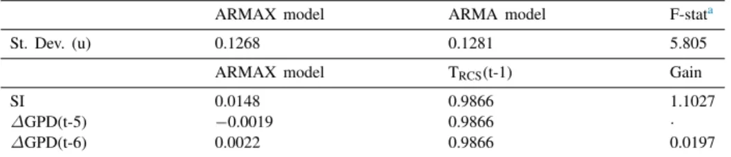
a counteracting effect on the above causal relationship. Nevertheless, the combined net effect is still positive. As regards the causality measures (Table 2) one can see that, despite the strength of the univariate component, the contribution of the exogenous factors SI and ∆GDP is 99% significant (F-statistics 5.805 > F critical value (3, 733) at the 0.01 significance level 3.808). The analysis of the multiplicative impacts (Table 2) shows that the steady-state gain G of SI is equal to 1.1, while that of ∆GDP is equal to 0.02; however, the gap is due to the fact that G depends on the unit of measure of the variables.
As regards the feedback effect of TRC S and SI on the human activity expressed by ∆GDP, the best-fitting
model is the ARX+ARCH because the series (bottom right panel ofFig. 1) exhibits strong heteroscedasticity. The departure from normality of the residuals (H0: errors are normally distributed, Chi-square (2df) 72.987, p-value
Fig. 2. (a) Normal distribution and (b) Q-Q plot of the residuals for the ARMAX model of Eq.(10).
Table 2. Causality statistics yielded by changes in the predictors for the model of Eq.(10).
ARMAX model ARMA model F-stata
St. Dev. (u) 0.1268 0.1281 5.805
ARMAX model TRCS(t-1) Gain
SI 0.0148 0.9866 1.1027
∆GPD(t-5) −0.0019 0.9866 ·
∆GPD(t-6) 0.0022 0.9866 0.0197
aF critical value (3, 733) at the 0.01 significance level: 3.808, p-value: 0.0006.
Fig. 3. (a) Normal distribution and (b) Q-Q plot of the residuals of the ARX+ARCH model Eq.(11).
0.0000) (Fig. 3) is a natural consequence. Notably, the model residuals are affected by many anomalous observations during a couple of periods, the first between the early 1300 s and mid-1400 s, the second between the mid-1500 s and early 1700 s (Fig. 4). On the whole, they correspond to a period that roughly overlaps with the so-called Little Ice Age. Once the model is re-estimated using the data subset from the year 1750 onward, the ARX+ARCH model is less affected by anomalous residuals and corroborates the results for the predictors TRC S and SI.
Fig. 4. Residuals (red line) and .95 Confidence intervals (blue line) for the ARX-ARCH model of Eq.(11).. (For interpretation of the references to color in this figure legend, the reader is referred to the web version of this article.)
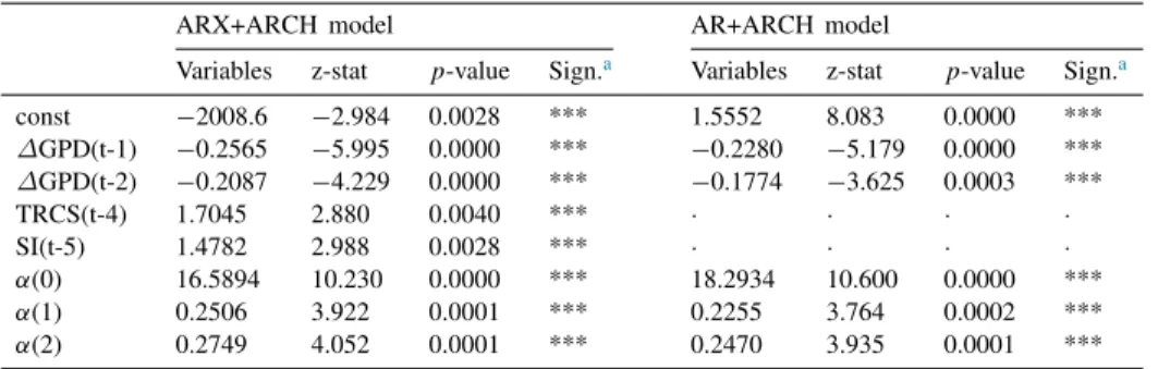
Table 3. Results for the model of Eq.(11), dependent variable ∆GPD. ARX+ARCH model AR+ARCH model
Variables z-stat p-value Sign.a Variables z-stat p-value Sign.a const −2008.6 −2.984 0.0028 *** 1.5552 8.083 0.0000 *** ∆GPD(t-1) −0.2565 −5.995 0.0000 *** −0.2280 −5.179 0.0000 *** ∆GPD(t-2) −0.2087 −4.229 0.0000 *** −0.1774 −3.625 0.0003 *** TRCS(t-4) 1.7045 2.880 0.0040 *** · · · · SI(t-5) 1.4782 2.988 0.0028 *** · · · · α(0) 16.5894 10.230 0.0000 *** 18.2934 10.600 0.0000 *** α(1) 0.2506 3.922 0.0001 *** 0.2255 3.764 0.0002 *** α(2) 0.2749 4.052 0.0001 *** 0.2470 3.935 0.0001 *** aSignificance levels: * 10%; ** 5%; *** 1%.
Table 4. Causality statistics yielded by changes in the predictors of the model(11).
ARX+ARCH model AR+ARCH model Likelihood-ratio testa
Log-likelihood −2290.1240 −2305.9910 31.734 ARMAX model TRCS(t-1) Gain
TRCS(t-4) 1.7045 0.4652 1.1633
SI(t-5) 1.4782 0.4652 1.0089
aChi-square critical value (2) at the 0.01 significance level: 9.2103, p-value: 0.0000.
The results (Table 3) suggest that both SI and TRC S exert a feedback effect on ∆GDP. Notably, the time lags
are as follows: five years in the case of SI and four years for TRC S, both with positive coefficients. That means that
the higher the temperature and solar irradiance is, the higher the gross domestic product is expected to be some years later. Due to the nonlinearity of the ARX-ARCH model and its ML estimation strategy, the causality nexus is tested using different measures (Table 4). However, the contribution of the exogenous factors SI and TRCS to ∆GDP is 99% significant (Likelihood-ratio test 31.734> Chi-square critical value (2) at the 0.01 significance level 9.2103). As far as the multiplicative impacts (Table 4) are concerned, the steady-state gain G of TRCS is equal to 1.2, while that of SI is equal to unity.
5. Conclusions
This study focuses on the cause-and-effect relationships occurring between economic growth and climate change, as well as on the feedback that the latter can provide for the former. After setting up the methodological framework
by which long time series of climate and economic data can be investigated, several model specifications have been tested. The ARMAX one provides valuable results in order to explain the trend of temperature anomalies and the role played by human factors. The ARX-ARCH one allows shedding light on the feedback effect exerted by climate change on growth and development.
In summary, we can conclude that the findings presented here support the occurrence of bi-directional causality between the analyzed phenomena. Two results are worth highlighting, in particular. On the one hand, one could state that climate change is a constant feature throughout the centuries, while human activities amplify global warming. On the other hand, climatic factors have a feedback effect on economic growth. Therefore, the challenge we are facing is to deal with climate change and take under control global warming, without hindering their positive feedback on human development.
Declaration of competing interest
The authors declare that they have no known competing financial interests or personal relationships that could have appeared to influence the work reported in this paper.
References
[1] Bar-Yosef O. Introduction: Some comments on the history of research. Rev. Archaeol. 1998;19:1–5.
[2] Diamond J, Bellwood P. Farmers and their languages: The first expansions. Science (80-. ) 2003;300:597–603.http://dx.doi.org/10. 1126/science.1078208.
[3] Richerson PJ, Boyd R, Bettinger RL. Was agriculture impossible during the pleistocene but mandatory during the holocene? A climate change hypothesis. Am Antiq 2001;66:387–411.http://dx.doi.org/10.2307/2694241.
[4] Gamble C, Davies W, Pettitt P, Richards M. Climate change and evolving human diversity in Europe during the last glacial. Philos Trans R Soc London Ser B Biol Sci 2004;359:243–54.http://dx.doi.org/10.1098/rstb.2003.1396.
[5] Bianchi GG, McCave IN. Holocene periodicity in North Atlantic climate and deep-ocean flow south of Iceland. Nature 1999;397:515–7.
http://dx.doi.org/10.1038/17362.
[6] Buntgen U, Tegel W, Nicolussi K, McCormick M, Frank D, Trouet V, Kaplan JO, Herzig F, Heussner K-U, Wanner H, Luterbacher J, Esper J. 2500 years of European climate variability and human susceptibility. Science (80-. ) 2011;331:578–82.
http://dx.doi.org/10.1126/science.1197175.
[7] Ljungqvist FC. A new reconstruction of temperature variability in the extra-tropical northern hemisphere during the last two millennia. Geogr Ann Ser A, Phys Geogr 2010;92:339–51.http://dx.doi.org/10.1111/j.1468-0459.2010.00399.x.
[8] Huntington E. Climatic change and agricultural exhaustion as elements in the fall of Rome. Q J Econ 1917;31(173).http://dx.doi.org/ 10.2307/1883908.
[9] Yasuda Y. The great east asian fertile triangle. In: Yasuda Y, editor. Advances in Asian Human-Environmental Research. Tokyo: Springer; 2013, p. 427–58.http://dx.doi.org/10.1007/978-4-431-54111-0_14.
[10] Lamb HH. The early medieval warm epoch and its sequel. Palaeogeogr Palaeoclimatol Palaeoecol 1965;1:13–37.http://dx.doi.org/10. 1016/0031-0182(65)90004-0.
[11] Grillenzoni C. Comparison of sequential monitoring methods for environmental time series with stochastic cycle. Environ Ecol Stat 2014;21:95–111.http://dx.doi.org/10.1007/s10651-013-0246-3.
[12] Jones PD, Mann ME. Climate over past millennia. Rev Geophys 2004;42.http://dx.doi.org/10.1029/2003RG000143, RG2002-1–42. [13] Neukom R, Steiger N, Gómez-Navarro JJ, Wang J, Werner JP. No evidence for globally coherent warm and cold periods over the
preindustrial common era. Nature 2019b;571:550–4.http://dx.doi.org/10.1038/s41586-019-1401-2.
[14] Goosse H, Arzel O, Luterbacher J, Mann ME, Renssen H, Riedwyl N, Timmermann A, Xoplaki E, Wanner H. The origin of the European Medieval Warm period. Clim Past 2006;2:99–113.http://dx.doi.org/10.5194/cp-2-99-2006.
[15] Ruddiman W. Plows, Plagues and Petroleum: How Humans Took Control of Climate. Princeton. ed.. Princeton University Press; 2005.
[16] Cook J, Oreskes N, Doran PT, Anderegg WRL, Verheggen B, Maibach EW, Carlton JS, Lewandowsky S, Skuce AG, Green SA, Nuccitelli D, Jacobs P, Richardson M, Winkler B, Painting R, Rice K. Consensus on consensus: a synthesis of consensus estimates on human-caused global warming. Environ Res Lett 2016;11:048002.http://dx.doi.org/10.1088/1748-9326/11/4/048002.
[17] Cook J, Nuccitelli D, Green SA, Richardson M, Winkler B, Painting R, Way R, Jacobs P, Skuce A. Quantifying the consensus on anthropogenic global warming in the scientific literature. Environ Res Lett 2013;8:024024. http://dx.doi.org/10.1088/1748-9326/8/2/ 024024.
[18] Tol RSJ. Comment on ‘quantifying the consensus on anthropogenic global warming in the scientific literature’. Environ Res Lett 2016;11:048001.http://dx.doi.org/10.1088/1748-9326/11/4/048001.
[19] Acaravci A, Ozturk I. On the relationship between energy consumption, CO2 emissions and economic growth in Europe. Energy 2010;35:5412–20.http://dx.doi.org/10.1016/j.energy.2010.07.009.
[20] Al-mulali U, Binti Che Sab CN. The impact of energy consumption and CO2 emission on the economic growth and financial development in the Sub Saharan African countries. Energy 2012;39:180–6.http://dx.doi.org/10.1016/j.energy.2012.01.032.
[21] Boontome P, Therdyothin A, Chontanawat J. Investigating the causal relationship between non-renewable and renewable energy consumption, CO2 emissions and economic growth in Thailand. Energy Procedia 2017;138:925–30.http://dx.doi.org/10.1016/j.egypro. 2017.10.141.
[22] Deviren SA, Deviren B. The relationship between carbon dioxide emission and economic growth: Hierarchical structure methods. Physica A 2016;451:429–39.http://dx.doi.org/10.1016/j.physa.2016.01.085.
[23] Dong K, Hochman G, Zhang Y, Sun R, Li H, Liao H. CO2 Emissions, economic and population growth, and renewable energy: Empirical evidence across regions. Energy Econ 2018;75:180–92.http://dx.doi.org/10.1016/j.eneco.2018.08.017.
[24] Le T-H, Quah E. Income level and the emissions, energy, and growth nexus: Evidence from asia and the Pacific. Int Econ 2018;156:193–205.http://dx.doi.org/10.1016/j.inteco.2018.03.002.
[25] Mikayilov JI, Galeotti M, Hasanov FJ. The impact of economic growth on CO2 emissions in Azerbaijan. J Clean Prod 2018;197:1558–72.http://dx.doi.org/10.1016/j.jclepro.2018.06.269.
[26] Rüstemo˘glu H, Andrés AR. Determinants of CO2 emissions in Brazil and Russia between 1992 and 2011: A decomposition analysis. Environ Sci Policy 2016;58:95–106.http://dx.doi.org/10.1016/j.envsci.2016.01.012.
[27] Saboori B, Sulaiman J, Mohd S. Economic growth and CO2 emissions in Malaysia: A cointegration analysis of the environmental kuznets curve. Energy Policy 2012;51:184–91.http://dx.doi.org/10.1016/j.enpol.2012.08.065.
[28] Salahuddin M, Alam K, Ozturk I, Sohag K. The effects of electricity consumption economic growth, financial development and foreign direct investment on CO2 emissions in Kuwait. Renew Sustain Energy Rev 2018;81:2002–10.http://dx.doi.org/10.1016/j.rser.2017.06. 009.
[29] Wang S, Li G, Fang C. Urbanization, economic growth, energy consumption, and CO2 emissions: Empirical evidence from countries with different income levels. Renew Sustain Energy Rev 2018;81:2144–59.http://dx.doi.org/10.1016/j.rser.2017.06.025.
[30] Acheampong AO. Economic growth CO2 emissions and energy consumption: What causes what and where? Energy Econ 2018;74:677–92.http://dx.doi.org/10.1016/j.eneco.2018.07.022.
[31] Mardani A, Streimikiene D, Cavallaro F, Loganathan N, Khoshnoudi M. Carbon dioxide (CO2) emissions and economic growth: A systematic review of two decades of research from 1995 to 2017. Sci Total Environ 2019;649:31–49.http://dx.doi.org/10.1016/j. scitotenv.2018.08.229.
[32] Shahbaz M, Solarin SA, Sbia R, Bibi S. Does energy intensity contribute to CO2 emissions? A trivariate analysis in selected African countries. Ecol Indic 2015;50:215–24.http://dx.doi.org/10.1016/j.ecolind.2014.11.007.
[33] Omri A, Nguyen DK, Rault C. Causal interactions between CO2 emissions, FDI, and economic growth: Evidence from dynamic simultaneous-equation models. Econ Model 2014;42:382–9.http://dx.doi.org/10.1016/j.econmod.2014.07.026.
[34] Han J, Du T, Zhang C, Qian X. Correlation analysis of CO2 emissions, material stocks and economic growth nexus: Evidence from chinese provinces. J Clean Prod 2018;180:395–406.http://dx.doi.org/10.1016/j.jclepro.2018.01.168.
[35] Box GEP, Jenkins GM. Time Series Analysis. Forecasting and Control. New York: John Wiley & Sons; 1976.
[36] White H. A heteroskedasticity-consistent covariance matrix estimator and a direct test for heteroskedasticity. Econometrica 1980;48(817).
http://dx.doi.org/10.2307/1912934.
[37] Engle RF. Autoregressive conditional heteroscedasticity with estimates of the variance of United Kingdom inflation. Econometrica 1982;50(987).http://dx.doi.org/10.2307/1912773.
[38] Granger CWJ. Investigating causal relations by econometric models and cross-spectral methods. Econometrica 1969;37(424). http: //dx.doi.org/10.2307/1912791.
[39] Grillenzoni C. Testing for causality in real time. J Econom 1996;73:355–76.http://dx.doi.org/10.1016/S0304-4076(95)01729-1. [40] Ahmed M, Anchukaitis KJ, Asrat A, Borgaonkar HP, Braida M, Buckley BM, Büntgen U, Chase BM, Christie DA, Cook ER,
Curran MAJ, Diaz HF, Esper J, Fan ZX, Gaire NP, Ge Q, Gergis J, González-Rouco JF, Goosse H, Grab SW, Graham N, Graham R, Grosjean M, Hanhijärvi ST, Kaufman DS, Kiefer T, Kimura K, Korhola AA, Krusic PJ, Lara A, Lézine AM, Ljungqvist FC, Lorrey AM, Luterbacher J, Masson-Delmotte V, McCarroll D, McConnell JR, McKay NP, Morales MS, Moy AD, Mulvaney R, Mundo IA, Nakatsuka T, Nash DJ, Neukom R, Nicholson SE, Oerter H, Palmer JG, Phipps SJ, Prieto MR, Rivera A, Sano M, Severi M, Shanahan TM, Shao X, Shi F, Sigl M, Smerdon JE, Solomina ON, Steig EJ, Stenni B, Thamban M, Trouet V, Turney CSM, Umer M, van Ommen T, Verschuren D, Viau AE, Villalba R, Vinther BM, Gunten LVon, Wagner S, Wahl ER, Wanner H, Werner JP, White JWC, Yasue K, Zorita E. Continental-scale temperature variability during the past two millennia. Nat Geosci 2013;6:339–46.
http://dx.doi.org/10.1038/ngeo1797.
[41] Bard E, Raisbeck G, Yiou F, Jouzel J. Solar irradiance during the last 1200 years based on cosmogenic nuclides. Tellus B Chem Phys Meteorol 2000;52:985–92.http://dx.doi.org/10.3402/tellusb.v52i3.17080.
[42] Brázdil R, Pfister C, Wanner H, Von Storch J. Historical climatology in Europe – the state of the art. Clim Change 2005;70:363–430.
http://dx.doi.org/10.1007/s10584-005-5924-1.
[43] Briffa KR, Bartholin TS, Eckstein D, Jones PD, Karlén W, Schweingruber FH, Zetterberg P. A 1, 400-year tree-ring record of summer temperatures in Fennoscandia. Nature 1990;346:434–9.http://dx.doi.org/10.1038/346434a0.
[44] Dahl-Jensen D. Past temperatures directly from the greenland ice sheet. Science (80-. ) 1998;282:268–71. http://dx.doi.org/10.1126/ science.282.5387.268.
[45] Graumlich LJ. A 1000-year record of temperature and precipitation in the Sierra Nevada. Quat Res 1993;39:249–55.http://dx.doi.org/ 10.1006/qres.1993.1029.
[46] Lean J, Beer J, Bradley R. Reconstruction of solar irradiance since 1610: Implications for climate change. Geophys Res Lett 1995;22:3195–8.http://dx.doi.org/10.1029/95GL03093.
[47] Mann ME, Zhang Z, Rutherford S, Bradley RS, Hughes MK, Shindell D, Ammann C, Faluvegi G, Ni F. Global signatures and dynamical origins of the little ice age and medieval climate anomaly. Science (80-. ) 2009;326:1256–60.http://dx.doi.org/10.1126/science.1177303. [48] Meeker LD, Mayewski PA. A 1400-year high-resolution record of atmospheric circulation over the North Atlantic and Asia. Holocene
[49] Neukom R, Barboza LA, Erb MP, Shi F, Emile-Geay J, Evans MN, Franke J, Kaufman DS, Lücke L, Rehfeld K, Schurer A, Zhu F, Brönnimann S, Hakim GJ, Henley BJ, Ljungqvist FC, McKay N, Valler V, von Gunten L. Consistent multidecadal variability in global temperature reconstructions and simulations over the common era. Nat Geosci 2019a;12:643–9. http://dx.doi.org/10.1038/s41561-019-0400-0.
[50] Trouet V, Esper J, Graham NE, Baker A, Scourse JD, Frank DC. Persistent positive North Atlantic oscillation mode dominated the medieval climate anomaly. Science (80-. ) 2009;324:78–80.http://dx.doi.org/10.1126/science.1166349.
[51] Zhang Q-B, Cheng G, Yao T, Kang X, Huang J. A 2, 326-year tree-ring record of climate variability on the northeastern Qinghai-Tibetan plateau. Geophys Res Lett 2003;30:2–5.http://dx.doi.org/10.1029/2003GL017425.
[52] Lean JL. Estimating solar irradiance since 850 CE. Earth Sp Sci 2018;5:133–49.http://dx.doi.org/10.1002/2017EA000357.
[53] Manley G. Central england temperatures: Monthly means 1659 to 1973. Q J R Meteorol Soc 1974;100:389–405.http://dx.doi.org/10. 1002/qj.49710042511.
[54] Manley G. The mean temperature of central england 1698–1952. Q J R Meteorol Soc 1953;79:242–61.http://dx.doi.org/10.1002/qj. 49707934006.
[55] Parker D, Horton B. Uncertainties in central England temperature 1878-2003 and some improvements to the maximum and minimum series. Int J Climatol 2005;25:1173–88.http://dx.doi.org/10.1002/joc.1190.
[56] Parker DE, Legg TP, Folland CK. A new daily central england temperature series, 1772–1991. Int J Climatol 1992;12:317–42.
http://dx.doi.org/10.1002/joc.3370120402.
[57] D’Arrigo R, Wilson R, Jacoby G. 2006a. Northern Hemisphere Tree-Ring-Based STD and RCS Temperature Reconstructions, IGBP PAGES/World Data Center for Paleoclimatology, Data Contribution Series # 2006-092. NOAA/NCDC Paleoclimatology Program, Boulder CO, US.
[58] D’Arrigo R, Wilson R, Jacoby G. On the long-term context for late twentieth century warming. J Geophys Res 2006b;111(D03103).
http://dx.doi.org/10.1029/2005JD006352.