UNIVERSITY OF SALERNO
R
ESEARCHD
OCTORATE INE
CONOMICS ANDM
ARKET ANDB
USINESSP
OLICIES(ECONOMIA E POLITICHE DEI MERCATI E DELLE IMPRESE)
Curriculum: Statistical Methods - XXX Cycle -
Equal Opportunities to Prosper:
A Statistical Analysis of Macro- and Microeconomic Factors
Candidate: Gianluca Mele Matricola n. 8801000002
Rapporteur : Ch.ma Prof.ssa Alessandra Amendola
INDEX
Introduction
Origin, scope, and features of this doctoral research ... 5
Synopsys of this work ... 6
Quick overview of statistical approaches used in this monograph ... 10
Chapter 1 “An Assessment of the Access to Credit - Welfare Nexus: Evidence from Mauritania”... 18
1. Introduction ... 18
2. The International Literature on Financial Access and Poverty ... 20
3. Methodology ... 22
4. Country context: Mauritania ... 24
4.1 Macroeconomic overview ... 24
4.2 Access to the Finance and Banking Sector ... 25
5. Household Characteristics, Poverty Incidence and Credit Access ... 28
6. Analytical Framework ... 33
6.1 Endogeneity of Access to Credit ... 34
6.2 Validity of the exclusion restriction ... 35
7. Results ... 40
8. Conclusions ... 45
Chapter 2 Do Nonrenewable Resources Support GDP Growth and Help Fight Inequality? ... 48
Introduction and Literature Review ... 49
Methodology ... 54
Data... 55
The Baseline Model: Pooling All Countries ... 63
Controlling for Heterogeneity between Income Groups ... 65
Analyzing a Subsample of Resource-Rich Countries ... 69
Conclusions ... 71
Chapter 3 Fiscal Incentive and Firm’s Performance. Evidence from Dominican Republic ... 74
Introduction ... 75
Literature review ... 77
Corporate Income Tax in the DR... 79
Data... 82 Methodology ... 83 Variables choice ... 86 Variables of Interest ... 87 Selected covariates ... 88 Treatment Indicator ... 90 Descriptive Statistics ... 90 Results... 91
Determinants of Fiscal Incentives ... 91
Types of Matching employed ... 93
Robustness and Balancing Test ... 94
Matching Balancing Test ... 96
Policy Conclusions... 99
Introduction
Origin, scope, and features of this doctoral research
Undertaking a doctoral research in economics and statistics had been part of my interests for a long time, immediately after the conclusion of my masters’ degree. Due to professional and personal factors, this project could only materialize a few years later, in the academic year 2014/15, when I joined the University of Salerno as a PhD student.
The main motive to start a doctoral research path for me was to strengthen my technical background and skills in statistics and quantitative economics. I have worked as a development economics professional since 2007, initially at the United Nations and more recently at the World Bank Group. In my work, I have dealt with economy policy issues on a daily basis; this often takes the form of economic diagnostics and policy advice resulting from an analysis of in-country specific issues as well as sourcing from international benchmarks and cross-country evidence. Against this background, developing a strong understanding of econometric and statistical approaches can indeed bring significant value added to my expertise, and provide me with more apt tools to operate as a well-rounded development economist.
This research path has also allowed me to be regularly in touch with the academic world, including other PhD candidates, research assistants, and faculties. This exchange over time has been extremely rich and greatly benefited the progression of my work. In addition, the possibility of publishing the results of my research activity on scientific statistical/economic peer reviewed journals, has represented a great opportunity, as it allowed me to contribute more meaningfully to foster opportunities for knowledge-sharing through academic platforms. In this respect, it seems worth noting that the first paper of this monograph was
accepted and published by the “International Journal of Business and Management”1, and that the second paper was accepted to the peer reviewing phase by the “Oxford Economic Papers” and currently awaits final feedback. The three chapters composing this monograph have also been individually presented at various national scientific conferences on statistics and economics in Italy, as well as they have all been published as work in progress under the World Bank Research Working Paper Series.
One of the main elements that has characterized this doctoral research project has been an in-depth country knowledge and hands-on development economics expertise. This means that in often cases, due my professional duties, I have had an opportunity to access to unique (and for the larger part, not public) datasets. This has added interest to the research and anchored it to concrete policy questions. This permitted to orient the research by actual facts rather than by goals with a high degree of abstraction. In conclusion, on of the leitmotivs of this monograph is that various statistical methodologies were selected and adapted to factual cases rather than the other way around, which adds policy relevance to the findings and makes the research especially meaningful.
Synopsys of this work
Societies strive to achieve socio-economic systems that provide equal and broad-based opportunities to their people. The concept of “equal opportunities” is a very complex one, and encompasses many definitions and several different areas of life. ‘Equal opportunities’ does not only mean to be able to access basic services and ideally with the same quality
standards; it may also mean to find a decent job and lead fulfilling professional lives, or also to thrive personally, without facing discriminations or – essentially – moving from the expectation that – if all people are indeed equal – conditions should be such that (while people cannot systematically have the same starting points in life) the resources available and the sociopolitical-economic principles that govern life may help level off the playing field, and provide a fair chance for success to all, without distinctions. Analyzing equality of opportunities has typically translated into the utilization of complex statistics, ranging from concentration indexes (e.g. the Gini coefficient) to sophisticated modeling of growth patterns, poverty outcomes, human behavior and social justice principles.
A quick overview on the main thinkers on inequality cannot fail to omit John Rawls. In his “Theory of Justice”2, Rawls asserts that nobody is truly
“created equal”, at least not from morally. Individuals are randomly born and unconsciously placed in various households, which reflect a number of differences related to gender, race, income, etc. Also, the socio-political institutions that may allow individuals to move along the spectrum of opportunities (and thus ‘equality’) are often reachable through financial means (e.g. schooling), which leads Rawls to highlight the important of social cooperation to mitigate such structural moral injustice. At the same time, Nobel Prize winner Amartya Sen, in his famous “Inequality Reexamined”3, put the accent on what type of equality a society seeks; to
do this, he delved into the diversity of mankind and their features. Sen asserts that, when we consider inequality, we should focus on the diversity among people’s capacities (so-called “capability approach”) and characteristics, rather than their welfare or financial means. In doing this,
2 Cfr. : “A theory of justice”, by John Rawls - Belknap Press of Harvard University Press
- 2003
Sen was among the first to look at inequality from the perspective of gender. An interesting angle is debated by John Roemer4, who distinguished a notion of time in the debate on equality. Roemer asserts that the concept of “equality of opportunity” is based on a ‘before’, i.e. ahead of the competition among individuals, and an ‘after’, i.e. when the competition has started. In the former segment, Roemer advocates for an equalization of opportunities, supported by policy interventions if needed, while in the latter segment, individuals should compete based on a nondiscrimination principle, and only on the qualities that are relevant to the competition in question (which means, excluding any other attributes such as sex, race, income, etc.).
T
he three papers presented in this monograph intend to discuss this question from selected and very distinct perspectives: 1) how (and if) financial access benefits peoples’ wellbeing; to do this we applied an econometric framework to a case-study based on Mauritania; 2) how natural resource endowment is correlated with economic growth and inequality indicators; in this case we adopted a global perspective and utilized a dataset covering over 40 countries; and 3) if tax incentives can be an effective tool in achieving economic growth in an way that does not distort competition among enterprises; also in this case we utilized a case-study approach, focusing on the experience of the Dominican Republic, to try and determine policy lessons.More specifically, the first paper presented in this monograph evaluates the impact of access to credit from banks and other financial institutions on household welfare in Mauritania. Household level data were used to evaluate the relationship between credit access, a range of household characteristics, and welfare indicators. In order to address the risks of potential endogeneity, an index of household isolation was used to
instrument access to credit. As we conducted the analysis, we also provided evidence on the validity of the exclusion restriction, by showing that household isolation is unrelated with households and area characteristics six years prior to the measurements on which this analysis is based. In a nutshell, results show that households with older and more educated heads are more likely to access financial services, as are households living in urban areas. In addition, the analysis shows that greater financial access is associated with a reduced dependence on household production and increased investment in human capital. The policy conclusions from our analysis appear to support public sector’s strategies for expanding financial infrastructures in underserved rural areas, as this is expected to translate into improved wellbeing for the local population.
In the second paper, the analysis examines the relationship between nonrenewable resource dependence, economic growth and income inequality. Using a dataset that includes information on 43 countries, going from 1980 to 2012, the paper estimates several model specifications in order to check the robustness of the results under many different assumptions. The analysis also accounts for income-group-related heterogeneity among countries, trying to understand whether structural characteristics of a nation (e.g. its institutional capacity, its development stage, etc., proxied in this case by the income level) can contribute to explain how growth, inequality, and resource endowment interact with each other. Innovating on a large strand of literature based on cross-sectional analysis, this second paper tackles the potential time invariant unobserved heterogeneity, thus exploiting the panel of the data. The findings show that the empirical relationships are associated with the level of economic development. Among higher-income countries, greater dependence is associated with lower income inequality, while no statistically significant correlation exists with GDP per capita. Among the
lower-income group, greater dependence is associated with both higher levels of income inequality and lower per capita GDP.
Finally, the third paper evaluates the impact of fiscal incentives on firms’ performance in the Dominican Republic. In recent years, the Dominican government has approved several new corporate tax benefits. While the literature on value-added tax incentives is extensive, the impact of corporate tax incentives is less well studied and is the subject of an ongoing debate. Using firm-level panel data from 2006 to 2015, this analysis uses a propensity score matching to investigate the relationship between tax incentives and firms’ performance, considering the measure of Liquidity, GFSAL, ROS, ROA, STS and Turnover as proxies of firms’ welfare. The results manage to single out the effect of tax expenditure and show – more specifically – that the Corporate Income Tax exemptions positively impacts the firms’ welfare. This evidence is corroborated both by a Nearest Neighbor Matching and a Radius Matching methodology, as well as it is supported by the balancing test.
Quick overview of statistical approaches used in this monograph
This monograph utilizes a wide range of statistical approaches to undertake economic analysis. This section will present the main ones, providing an overview on their main characteristics as well as advantages and/or limitations.
First of all, the analysis makes ample use of descriptive statistics. Descriptive statistics are very diverse techniques that are used to describe the basic characteristics of a dataset. Descriptive statistics provide a simple synthesis of the sample and of the measurements collected. Together with simple graphic analysis, they represent the initial starting point for any quantitative data analysis. Descriptive statistics should not be confused with inferential statistics. While the former are mostly
presenting a description of what is being observed or what the main data traits are, the latter will try to reach conclusions that extend beyond the data collected and which can be to some extent valid also beyond the specific study or experiment that concretely motivated them. In other words, descriptive statistics represent and synthesize a set or sample of data relating to a given population (‘population’ should be intended as the totality of cases, i.e. all the units on which a variable of interest can be detected).
This study also widely utilizes regression analysis as a technique used to exploit a set of data that consists of a dependent variable and one or more independent variables. The purpose of regression analysis is to estimate a possible functional relationship between the dependent variable and the independent variables. In short, the dependent variable (in the regression equation) is a function of independent variable(s) plus an error term. This latter is a random variable and represents an unmanageable and unpredictable variation in the dependent variable. A number of control variables or parameters are typically also estimated to best describe the dataset. One of the most commonly used methods in the regression analysis is the "least squares" (OLS) approach, although several other methods are also used. The essential advantage of regression analysis is that it can be used to make predictions, as well as to test hypotheses, or to model dependency relationships. The analysis in this monograph also utilizes two among the main alternatives to the pooled OSL model, the Fixed Effects Model, and the Random Effects Model.
Looking at the fixed effects model, the main concept is fundamentally that it is possible to break the error term u (i.e. all non-observable variables), in two components, ε and α :
Where α is the part of the error dependent on the observed unit(s), including the effect of all non-observable variables, and ε is the part of the peculiar error of the observation. The fixed effects model essentially focuses on the elimination of the α intercept5, constant over time, as it
contains non-observable values and would therefore be considered an integral part of the model error. These values could be correlated with the explanatory variables x(it), returning a distorted estimate. Excluding the term αi is achieved based on a data demeaning process6. Also the random
effects model, like the fixed effects model, breaks down the error term u(it) into two components ε(it) and α(i). However, an intercept is explicitly introduced in the model:
𝑦(𝑖𝑡) = β(0) + β(1)𝑥(𝑖𝑡,1) + ⋯ + β(𝑘)𝑥(𝑖𝑡,𝑘) + α(𝑖) + ε(𝑖𝑡)
So that it is possible to assume that that E(αi) = 0. In the fixed effects model we try to exclude the term α(i), as that is supposed to be correlated with one or more explanatory variables. Assuming that α(i) is not related to any explanatory variable in all t periods, any modification that excludes the term α(i) would lead to an inefficient estimator. When we use a random effects model, unlike the fixed effects model, α(i) is not treated as a fixed variable(s), but as a random one (which explains why the designation of “random effects”), which are not correlated to the regressors. By doing this, these effects can be treated in the model as if they were part of the error term. The next step is thus processing data and obtaining a dataset with non-autocorrelated errors. Since the processed data satisfy the assumptions of the Gauss-Markov's theorem, and the final estimates/results can be regarded as efficient.
The “Seemingly Unrelated Regression Equation” is another estimator that this monograph utilizes. It represents a linear regression model consisting
5 Given a function 𝑦(𝑖𝑡) = 𝑥(𝑖𝑡)𝛽 + 𝛼(𝑖) + 𝜀(𝑖𝑡)
6 which consists of subtracting the group mean from each of the variables and in
of several equations, each of which has their own dependent variables. Each of these equations may be estimated individually, and may also have different explanatory variables. This is the reason why the model is called “seemingly unrelated”. However, the error terms are assumed to be correlated across the various equations. In other words, the M equations may result to be “unrelated” in the sense that no simultaneity exists among the variables in the system as well as that each of the equations have their very own explanatory variables. The various equations would still be probabilistically correlated, by means of the errors that are correlated throughout the model’s equations.
The SURE can be regarded as a model made up of “M” multiple regression equations of the following form:
where y(ti) is the tth observation on the ith dependent variable (to be explained by the ith regression equation). The term x(tij) represents the tth
observation in jth explanatory variable, while β(ij) is the coefficient
associated with x(tij) for each observation, and finally ε(ti) is the tth value of the disturbances component associated with the equation under consideration (i.e. ith ). Summarizing, one could think of the SURE model as a very specific case of simultaneous M equations, with M jointly dependent variable and k distinct exogenous variables, and in which no endogenous variables appear as explanatory in any of the structural equations.
The first paper presented in this monograph largely resorts to the use of Instrumental Variable (IV), which is one of the most important and applied techniques used in econometrics. The main advantage – and reason why – the researcher utilizes IVs is endogeneity, which means that the researcher realizes the possibility that endogenous variables that are
influenced by other variables within the model, may be present. In other words, the risk would be that then, the regression estimates may measure just the magnitude of association, instead of the magnitude and the sign of the causation (which is what we need for policy analysis). If we consider a dependent variable y and a single regressor x, the instrumental variable (or more simply the “instrument”) can be defined, as “z”, which has the property that any changes in z will be reflected in changes in x, but will not lead to any changes in y. Consequently, z will be uncorrelated with the error terms u. The following diagram can help summarizing this definition:
In more formal terms, given a scalar regression model with the following form:
y = βx+u
a variable z is called an instrument or instrumental variable for the regressor x , if it respects two conditions: a) it must be uncorrelated with the error term u; and b) it is correlated with the regressor x. More specifically, the first condition guarantees that the selected instrument z is also a regressor in the model for y, because if y depended on both x and z and y is regressed on x alone then z would be absorbed into the error term, and consequently z would be related with the error term. The second condition simply states that there must be some level of correspondence between the instrument and the variable being instrumented. One main advantage of the IV estimation is that (like the “Propensity Score Matching” that will be described right after), IVs can fine-tune the model for both observed and unobserved confounding effects, which means that they come on help when there are conditions that may influence both the dependent variable and independent variable, thus causing a spurious
association. Other statistical approaches exist for adjusting for confounding effects, such as the stratification or the multiple regression methods, however these cannot adjust for unobserved confounders. This is what makes IVs particularly helpful in actual/factual applications, when the researcher is investigating matters related to observational data, which are likely indeed to be influenced not only by observed confounders but – in particular – by nonobservable ones. To conclude, one should note that IVs are better suited as an estimator technique when the sample size is sufficiently large. In addition, if the instrument is weak and/or if the relevance of confounders is large (or both) it is likely that the resulting standard errors will also be significant, which would translate into imprecise and biased results. Therefore, IVs are preferably to be used when only moderate to little confounding effects are assumed to exist. As previously mentioned, also the Propensity Score Matching is mostly used to analyze the causal effect of a treatment using observational data. In other words, the dataset is not generated by an experiment (so-called randomized) but was collected through surveys, experiments, and/or administrative records; this last case is the one of the third paper in this monograph. Matching procedures are used in those situations when the researcher wishes to estimate the impact of a given treatment on a certain output. A large literature exists on the conceptual problems related to the assessment of the impact of a treatment through microeconometric instruments (essentially individual-level surveys), and it points out to fundamental mismeasurement potential issues. For example, one of the most common limitations in this sense is the “self-selection”. A typical example is that of an individual enrolling in vocational training. It is likely that this individual carries more motivated than a number of individuals who do not enter the program. This is to say that, while – in an ideal world – assessing a casual treatment effect should be operated by calculating the average difference between the outcomes by the participants after
treatment and the potential that they would have achieved assuming (theoretically) that they had not received the treatment, in the actual world, it is possible to obtain information about the outcome of the treated individuals and the about the outcomes from a second group of individuals who did not receive the treatment. The Propensity Score Matching comes in help to solve these methodological issues: if a matching process allowed each individual (observed in the treatment group) to be associated with an individual in the untreated group that has the most (possible) resembling pre-treatment features, then the limitations described above would be – at least to a certain extent – excluded or reduced. In order to do this, it is important that two conditions are respected. The first condition is that the vector of variables on which the matching (x) is going to be conditioned, should be independent from the treatment. The second condition is that also the output distribution (conditioned by the set x) is independent from the treatment. More specifically, this second condition is known in the literature as “CIA” (that is, Conditional Independence Assumption) and is indeed of crucial importance, since only if the CIA is respected the selection of individuals can be expressed as a function of pretreatment features exclusively. The typical situation faced by micro-economists is that in which three variables of interest X, Y, Z are used, but the database in use does not contain (at all, or just partly) any joint observations of these three variables. Let us suppose that two distinct surveys exist, one containing the variables X and Y, and the other one containing X and Z. In order to integrate the two datasets, the researcher can assume that the information contained in X is adequate to determine both Y and Z; in other words, we move from the assumption that Y and Z are independent vis-à-vis X; i.e.:
P (Y, Z | X) = P (Y | X) P (Z | X),
which is a hypothesis entirely equivalent to the CIA. The next step is to define a criterion (or a set of criteria) to match the variable Z (that is
associated with an individual in the second group, which is most similarly conditioned by a set of common variables X) to each individual in the first group. This process is clearly more efficient than undertaking a new survey (whether at all possible) that would contain all the variables in an integrated database. Ultimately, the propensity score of a unit (may this be treated or untreated) is essentially the probability that a unit is assigned to the treatment given its characteristics prior to treatment. More formally this can be expressed as follows:
supposing that we have a binary treatment T, an outcome Y, and background variables X.While most of the literature on ‘score matching’ has essentially been developed as a response to an impact assessment of economic treatments, more recently the interest on such statistical approaches has also grown in other sectors, as this type of procedures allows to integrate information from different sources in a relatively simple fashion.
18
Chapter 1:
“An Assessment of the Access to Credit - Welfare
Nexus: Evidence from Mauritania”
7Keywords Access to Credit; Household Isolation Level; Instrumental Variable; Residuals
1. Introduction
The international literature on financial access and development has not yet identified a direct, unequivocal connection between household-level credit and improvements in poverty and inequality indicators. For example, Beck, Demirgüç-Kunt, and Levine (2007) found that financial access is correlated with lower rates of poverty and income inequality, while Honohan and King (2012) showed that the use of formal banking services is associated with an increase in individual monthly income. The World Bank’s Global Financial
7This analysis was conducted jointly with Alessandra Amendola, Marinella Boccia, all affiliated to the University of Salerno.
19 Development Report of 2014 finds that financial inclusion plays a central role for development and poverty reduction. Considerable evidence shows that the poor benefit significantly from basic payments, savings, and insurance services; however it also highlights that microcredit experiments draw a mixed picture about the development benefits of microfinance projects targeting specific population groups.
Many studies have focused on the role of microfinance in poverty reduction, and again the positive evidence on welfare is encouraging. (Note 1)Moreover, given the locally specific nature of both poverty dynamics and microfinance institutions, evidence is difficult to compare across cases, and there is no consensus regarding the effect of microfinance on growth and inequality. Illustrating the complexity of isolating the direct antipoverty effects of microfinance, Morduch (1998) found that “the most important potential impacts [of microfinance] are thus associated with the reduction of vulnerability, not of poverty per se, [because] the consumption-smoothing [effect] appears to be driven largely by income-smoothing, not by borrowing and lending”.
This paper contributes to the literature on the impact of financial access, as measured by credit from banks and other financial institutions (Note 2), on household welfare in Mauritania. The potential endogeneity of access to credit is addressed using an instrumental variable approach. The analysis draws on data from the Ongoing Survey of Household Living Conditions (Enquête Permanente sur les Conditions de Vie des Ménages, EPCV) implemented by the National Statistics Office (Office National de la Statistique, ONS). The 2014 EPCV covered 9,557 households across 13 regions (walleyes), 53 provinces (moughatas) and 647 districts.
20 The Mauritanian credit market is shallow, fragmented and overwhelmingly informal. Few formal credit providers operate in Mauritania, and most bank branches, ATMs and other financial infrastructure is confined to the capital, Nouakchott. There are also important cultural barriers to credit access— including a strong gender dimension—as well as pervasive information asymmetry between potential borrowers and lenders, and a generally poor legal and governance framework. Mauritania’s informal financial sector is extensive, but produces little reliable data. Informal finance is typically offered on simple terms and frequently involves family connections, tribal affiliations or other networks of social trust. Due to data limitations this analysis concentrates exclusively on the formal credit sector.
Among the limitations of this paper is the lack of panel data. Comparing the evolution of agents over time would add valuable information; however, current data do not allow the exploitation of longitudinal dimension. For future research to address these shortfalls, it will be critical to enhance the quality and the availability of official data. In this respect, a strong political commitment and consequent financial engagement to prioritizing statistics are key prerequisites for the revitalization of the analytical efforts that can support decision-makers improving the nexus between financial access and welfare.
2. The International Literature on Financial Access and Poverty
Most research on the relationship between financial access and poverty relies on standard welfare indicators such as household consumption, expenditure and income. Some studies show that the use of formal banking services increases individual monthly income (Honohan and King 2012), while others find that financial access is associated with lower rates of poverty and
21 inequality, inferring that the use of financial services has a disproportionately positive impact on the poor (Beck, Demirgüç-Kunt and Levine 2007). There is also evidence that financial access is linked to improvements in the severity of poverty (Honohan 2004). Research conducted in Pakistan and India reveals that the expansion of rural financial services is associated with improvements in household welfare (Khandker and Faruqee 2003) and that the development of bank branches increases non-agricultural economic output and reduces rural poverty (Burgess and Pande 2003).
Microfinance has been hailed as a vital tool for the economic empowerment of poor households. Research has shown that access to microfinance correlates with rising household income and consumption levels, less severe income inequality and enhanced welfare (Mahjabeen 2008). Studies have found a positive relationship between household characteristics, borrowing patterns and expenditure levels (Giang et al. 2015). Substantial research has focused on the issue of endogeneity in access to credit, and studies have shown that access to credit significantly influences economic incentives at the household level, improving consumption (Pitt and Khandker 1998) and altering positively consumption and investment decisions and impacting rates of wage growth and capital formation (Kaboski and Townsend 2012).
However, not all studies have found a positive correlation between financial access and improved poverty indicators. Some analyses have failed to show a relationship between microfinance and household welfare, and find that access to credit has a limited impact on per capita incomes, food security and on the nutritional status of credit program beneficiaries (Diagne and Zeller 2001). Others have revealed a regressive distribution of benefits (Mosley and Hulme 1998). Moreover, methodological issues remain a serious concern. According to Desai, Johnson and Tarozzi (2014), “Many proponents claim
22 that microfinance has had enormously positive effects among borrowers. However, the rigorous evaluation of such claims of success has been complicated by the endogeneity of program placement and client selection, both common obstacles in program evaluations. In this context randomized control trials provide an ideal research design to evaluate the impact.” In an effort to increase the analytical rigor of financial access studies, researchers turned to randomized controlled trials. This methodology has been used to estimate the impact of access to microcredit by comparing outcomes among a random sample of individual borrowers to those of non-borrowers with similar socioeconomic characteristics. Some of these studies have found that access to finance produced measurable benefits in the form of increased employment and food consumption (Karlan and Zinman 2010), other have displayed a significant impact on investment by small business, on profits by pre-existing businesses, as well on expenditure in durable goods, but not on consumption (Banerjee, Duflo, Glennerster and Kinnan 2015). Overall, these studies provide strong empirical evidence for a positive correlation between access to finance and household welfare.
3. Methodology
Causal conclusions of this work rely on the ability to instrument for access to credit. (Note 3) More in general: “Microfinance institutions (MFIs) typically choose to locate in areas predicted to be profitable, and/or where large impacts are expected. In addition, individuals who seek out loans in areas served by MFIs and that are willing and able to form joint liability borrowing groups (a model often preferred by MFIs) are likely different from others who do not along a number of observable and unobservable factors. Until recently, the
23 results of most evaluations could not be interpreted as conclusively causal because of the lack of an appropriate control group” (Desai, Johnson and Tarozzi 2014). In the absence of an experimental design, this issue is addressed by using the household isolation level (HIL) to instrument for access to credit. HIL is defined by using a number of indicators – self-reported by households – on the distance from various institutions and service providers. We assume that credit institutions have approximately the same average distance from households, and on these bases we move to estimate the relationships between access to credit and (i) consumption of household production, (ii) household total spending on non-durable goods and services, (iii) food spending, (iv) education spending and (v) poverty incidence.
The exclusion restriction states that the HIL affects household welfare only through its effects on access to credit. The validity of such restriction is ensured by controlling for all unobservable variables through area-level fixed effects. Unfortunately, data limitations in the panel structure of the dataset prevented us from using household-level fixed effects or longitudinal information to address the endogeneity problem. Nevertheless, this analysis provides evidence in favour of the exclusion restriction, showing that the exogenous variability was unrelated with households and with local patterns six years prior to the measurements on which this analysis is based.
24
4. Country context: Mauritania
This section provides a broad overview of the country’s characteristics and describes the patterns of the banking sector and access to finance.
4.1 Macroeconomic overview
Mauritania is a Sahelian country on the West Coast of Africa with a land area of approximately 1 million square kilometers, most of which is covered by the Sahara desert, and a population of roughly 3.6 million. (Note 4) The country has urbanized rapidly since the 1960s, and its population is now largely concentrated in Nouakchott and other major cities such as Nouadhibou and Rosso.
Mauritania has experienced robust growth in recent years driven by a thriving natural resource sector and high international commodity prices. However, recent global price shocks have underscored the country’s high degree of external exposure, which is magnified by a lack of diversification. Mauritania also faces exogenous vulnerabilities related to its ecology and geography, which make it especially sensitive to climate change, and it has a history of political instability, which is exacerbated by an inherently volatile system of tribal loyalties, an informal racial hierarchy, the rise of Islamic fundamentalism in the Maghreb region and persistent tensions with Morocco over Western Sahara.
Poverty is most pervasive and extreme in rural Mauritania, with some of the highest rates registered in the southern regions bordering Senegal. While overall poverty is declining, a combination of continued rural-urban migration and the volatility of the resource-based urban economy may be causing a gradual increase in urban poverty. Nevertheless, most of the country’s poor are concentrated in rural areas. (Note 5)About 30 percent of those aged 15-34 are not enrolled in school and do not participate in the labor
25 force. The capital-intensive mining sector is unable to absorb a rapidly growing number of low-skilled workers, and about 85 percent the labor force is employed in the informal economy, particularly semi-subsistence agriculture. (Note 6)
An adverse business and investment climate undermine Mauritania’s economic competitiveness, slowing the growth of its small formal sector and inhibiting diversification. In the mid-2000s Mauritania’s manufacturing and retail trade sectors included fewer than 250 formal firms with more than 5 employees. (Note 7) Burdensome procedures for paying taxes, resolving insolvency, starting a business, trading across borders and obtaining credit all present serious obstacles to formalization and expansion, particularly for small and medium enterprises (SMEs).
4.2 Access to the Finance and Banking Sector
The World Bank’s Doing Business report cites access to finance as the top constraint on the Mauritanian private sector. (Note 8) The banking industry is dominated by a few very large firms, which concentrate almost exclusively on serving specific commercial and industrial groups. Prospective borrowers who do not belong to these groups face considerable difficulty in accessing financial services. (Note 9) Major firms also tend to enjoy strong political connections, which they can use to protect themselves from competition. As a result of regulatory barriers and governance issues Mauritania ranked 168th
out of 189 countries in the 2016 Doing Business report.
The 2016 Doing Business report ranked Mauritania 162nd out of 189 countries in terms of the ease of getting credit, and its scores on several other financial indicators compare poorly with the average for Sub-Saharan Africa and most comparator countries. Information asymmetry is a major obstacle to financial access, especially for SMEs, as few prospective borrowers are able to present
26 a verifiable credit history. While credit to the economy has grown rapidly, increasing by 300 percent between 2005 and 2014, financial deepening in Mauritania has been far slower than in peer countries. The financial system is dominated by banks, and its structure evolved significantly in recent years, following the establishment of the state-owned Deposit and Development Fund (Caisse de Dépôts et de Development, CDD) in 2011, and the entry of several new commercial banks, some foreign-owned.
The small size, shallowness and fragmentation of the Mauritanian financial system are major impediments to the development of financial intermediation services. The assets of the country’s largest bank amount to just US$320 million, and total banking-sector assets are estimated at less than US$2 billion. Financial infrastructure is limited, and cash remains the most common means of payment in the domestic economy. The insurance industry and pension schemes play a very minor in the financial system, and the ability of banks to play a decisive role in supporting private-sector development is limited by nonperforming loans, which remained high at over 20 percent of total loans in 2013, though down from 45 percent in 2010.
In 2013 banking-sector assets represented 38 percent of GDP, and credit to the private sector represented 26 percent. (Note 10) The return on assets stood at 2 percent, and the return on equity was 9 percent. In recent years interest rates on credit declined from 15 percent to 10-12 percent as new banks entered the market. However, rates vary little based on counterparty, maturity or type of financing. Headline profitability is mediocre, limiting both the sector’s potential for organic growth and its capacity to absorb shocks. The absence of a market for short-term liquidity is a major impediment to the development of intermediation. Indicators of access to financial services in Mauritania remain below the average for Sub-Saharan Africa.
27 The country’s microfinance sector is similarly underdeveloped. In 2013 there were 31 registered microfinance institutions (MFIs) in Mauritania, 10 of which were in the process of losing their licenses. Most MFIs are small, and the country currently has only one large microfinance network, the Public Credit and Savings Fund Promotion Agency (L'agence de Promotion des Caisses Populaires d'Epargne et de Crédit, PROCAPEC). Nevertheless, the total number of MFI clients increased from 139,000 in 2006 to over 200,000 in 2014, and MFIs now account for about 5 percent of all loans and 2 percent of all deposits. MFI loan maturities range from 3 months to 2 years, and rates for small businesses average 16 percent. MFIs also provide savings accounts—though these are limited to very short-term non-remunerated deposits—and offer money transfers. Islamic financial products are common, especially non-interest-bearing rent-to-own agreements (murabaha), which represent over 74 percent of PROCAPEC loans.(Note 11)
Mauritania’s financial sector also faces challenges relate to its geographic isolation, hard infrastructure gaps and general lack of technical capacity. Bank credit to the private sector is overwhelmingly short-term, and information asymmetry severely limits its allocative efficiency. Lack of information about potential borrower leads banks to disregard SMEs in favor of large, well-established firms. As a result, informal financing, including at the international level, is often the only option available for Mauritanian SMEs. Low individual bancarization rates represent a major additional constraint on credit access. Information technology is limited, clearing systems mostly rely on manual entry, and electronic payment instruments are seldom utilized. The government recently began preparing a credit card system in collaboration with the private sector, but this effort is still in its early stages. Finally, weak legal and judicial systems inhibits the enforcement
28 of contracts, and the legislative framework for protecting creditors’ rights is virtually nonexistent.
5. Household Characteristics, Poverty Incidence and Credit Access
The analysis presented below is based on the Mauritania EPCV for 2014. The survey is the result of a partnership between the ONS, the Ministry of Economic Development, the World Bank, and Afristat. The survey covers a wide range of socioeconomic variables collected through questionnaires administered to households and communities. The “basic indicators of wellbeing” module contains data on household composition, labor, education, social capital, health, access to services and credit. The “revenue and expenditure” module includes information on spending, consumption, transfers and income. The household represents the statistical unit of analysis. Of the 9,557 households surveyed in the 2014 EPCV, 55.3 percent were in urban centers and 44.7 percent were in rural areas. As a secondary source of information, the analysis is based on data from the 2008 EPCV. This household survey shares the same structure as the 2014 one, and consists of 13.738 households. The two surveys are cross-sectional representative samples of the underlying population. In the following paragraphs, a number of descriptive statistics set the stage for the main empirical analysis, which will be presented in the next section.
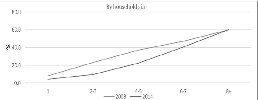
Mauritanian households are generally organized according to a traditional patriarchal model. Sixty-eight percent of households are headed by men, and 32 percent are headed by women. Household size is clearly correlated with poverty, and poverty incidence increases linearly with the number of household members. Households headed by married people tend to both include more children and are poorer than households headed by single
29 people. Polygamy is relatively common in Mauritania, and polygamous households tend to be among the largest and poorest in the country. Poverty rates declined among all household types between the 2008 and 2014 surveys, with medium-sized households showing the greatest degree of improvement (Figure 1).
Figure 1. Poverty Incidence by Household Size
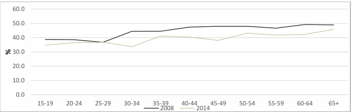
The poverty incidence does not appear to depend on the gender of the household head. Male-headed households tended to be marginally poorer both in 2008 and 2014, even when controlling for household size. The age of the head of household also appears to have no effect on poverty levels. Welfare indicators improved among all age groups in 2014, but households headed by younger people showed a more markedly positive trend (Figure 2).
30
Figure 2. Poverty Incidence by Age Group of Household Head
Households headed by public employees had the lowest poverty rates. Households headed by private employees had higher rates, followed by households headed by self-employed workers outside the agricultural sector. Households headed by self-employed workers in the agricultural sector were the poorest, and their poverty incidence was even higher than that of households headed by unemployed workers or non-participants in the labor force. Finally, households headed by unemployed individuals registered an increase in the incidence of poverty, likely reflecting a severe drought that hit the country in 2012 (Figure 3).
0.0 10.0 20.0 30.0 40.0 50.0 60.0 15-19 20-24 25-29 30-34 35-39 40-44 45-49 50-54 55-59 60-64 65+ % 2008 2014 0.0 10.0 20.0 30.0 40.0 50.0 60.0 70.0 80.0
Public employee Private employee
Self-employed agriculture
Self-employed non agriculture
Family aids Unemployed Inactive 2008 2014
31
Figure 3. Poverty Incidence by Occupation
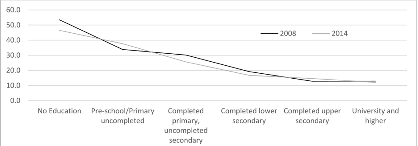
The education level of the head of household is negatively correlated with poverty incidence. Primary education is compulsory in Mauritania and lasts 6 years. Secondary school covers a period of 6 or 7 years, depending on whether the student opts for a Professional or Technical Baccalaureate, or a full Baccalaureate. Tertiary education typically lasts 3-6 years; advanced degrees are very rare and are usually obtained from the University of Nouakchott. In addition to the formal school system, traditional qur’anic schools (madrasas) are common in Mauritania. Figure 4 shows the negative correlation between education and poverty at the household level.
Figure 4. Poverty Incidence by Education Level of Household Head
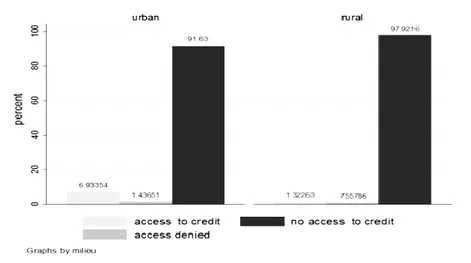
Most importantly for the aim of this research, very few Mauritanian households have access to credit, and bank presence is almost exclusively restricted to urban areas. The EPCV includes questions designed to gauge household demand for credit during the 5 years prior to the survey. Figure 5 shows the share of households that have applied for credit from a formal financial institution, as well as the share that had their requests approved. Households applying for credit represent a tiny fraction of the population at
0.0 10.0 20.0 30.0 40.0 50.0 60.0 No Education Pre-school/Primary uncompleted Completed primary, uncompleted secondary Completed lower secondary Completed upper secondary University and higher 2008 2014
32 just 5.6 percent, down from 8.8 percent in 2008. However, the likelihood of a successful credit application increased between the two surveys, rising from 3.23 percent in 2008 to 4.45 percent in 2014. Credit applications are far more common, and credit approval is far more likely, among urban households as opposed to their rural counterparts (Figure 5). Physical access to banks is even more heavily skewed in favor of urban households, about a quarter of which have access to a bank, compared to just over 1 percent of rural households (Figure 6).
Figure 5. Credit Demand by Area
33
6. Analytical Framework
A comprehensive understanding of household welfare requires an analysis of both income and consumption patterns. Income shocks do not always directly translate into decreased consumption or diminished welfare, and the mitigating factor may be thought of as household resilience. The ability to draw on past savings, to fall back on public assistance or to access credit to address temporary income shocks are all dimensions of resilience. Reflecting a long strand of literature (Note 12) on the importance of consumption rather than income as a primary indicator of household welfare, and taking into account the role of resilience, the analysis considers the following welfare indicators: (i) consumption (Note 13) of household production, particularly agricultural produce; (ii) total spending on nondurable goods, excluding food and education; (iii) food spending; (iv) education spending; and (v) a dummy variable representing household poverty status.
The following equation defines the parameters of interest:
Υi = α∁i + ∑Vv=1δvΧv,i + μi + εi. (1)
Where Υ𝑖 is a dependent variable indexed to i (household) and ∁𝑖 is the dummy variable indicating whether the household has accessed credit from a formal financial institution in the five years preceding the interview. In addition, Χ𝑣,𝑖 represents a set of 𝑉 = 14 households characteristics, including
the number of male adults in the household, number of children, total household size, amount of land owned, and dummy variables for urban or rural location, gender, age and education level of the household head. Area-level fixed effects by province (moughata) are represented by 𝜇𝑖, and 𝜀𝑖 is an
error term - which is allowed to be heteroskedastic in the analysis. Standard errors are clustered on moughata. (Note 14)
34 6.1 Endogeneity of Access to Credit
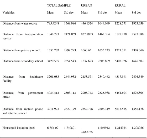
The estimation of (1) is most likely affected by the endogeneity of access to credit. This may be due to a number of factors, including: (i) unobserved area-level fixed effects that influence both demand for credit and household income and consumption, such as local prices, infrastructure quality, cultural norms, environmental conditions and natural-disaster risks; and (ii) unmeasured household characteristics that affect both demand for credit and household income and consumption, such as the health, ability, and fecundity of household members, as well as preference heterogeneity. (Note 15) An instrumental variable strategy (IV) based on the concept of the household isolation level (HIL) is used to address the endogeneity problem. The HIL (denoted by Ζ𝑖 in what follows) is computed by considering the average value of a household’s distance from vital infrastructure and facilities. These include the nearest water source, primary and secondary school, government offices, transportation services, healthcare facilities, mobile phone and internet services. Results are robust to alternative sets of variables considered to compute the HIL index. (Note 16)
Table 1 shows the descriptive statistics for this indicator, along with the various components which contribute to its definition. The first two columns report the mean (in meters) and the standard deviation from the full sample. The two central columns report these same statistics for households in urban areas, while households living in rural areas are considered in the last two columns of the table.
The results show that the age, the education level of the household head as well as the household’s location (whether in an urban area or not) appear to be significant determinants of credit access. Moreover, households that
35 successfully obtain credit tend to be less dependent on the consumption of household internal production and are more likely to invest in education.
Table 1. Descriptive Statistics for the proxies Household Isolation Level (HIL)
TOTAL SAMPLE URBAN RURAL
Variables Mean Std dev Mean Std dev Mean Std dev
Distance from water source 795.4248 1569.986 446.1524 1049.099 1228.571 1953.639
Distance from transportation service
1848.723 2421.069 827.8833 1462.304 3128.778 2573.088
Distance from primary school 1353.707 1999.793 1060.65 1655.723 1721.311 2308.066
Distance from secondary school 3420.595 2654.543 1837.693 2206.809 5403.926 1646.502
Distance from healthcare facility
3201.083 2644.932 2153.571 2340.462 4517.591 2404.349
Distance from government office
4034.412 2503.113 2905.743 2525.988 5454.604 1576.805
Distance from mobile phone and internet service
3911.923 2629.179 2552.726 2606.349 5615.555 1356.178
Household isolation level 6.75e-09 1.740801 -.9687785
1.469942 1.214924 1.208036
6.2 Validity of the exclusion restriction
The HIL index is regarded as a determinant for access to banks and other financial institutions. (Note 17) The location of household in rural and urban areas may follow from sorting along unobservable dimensions. Because of this, household isolation can be itself endogenous in our model, thus invalidating the exclusion restriction needed for identification. The instrumental variation employed here is the residual variability in HIL after
36 netting off area unobservables and characteristics of the households living in those areas.
To see this, the first stage equation is:
∁i = βΖi+∑Vv=1γvΧv,i + μi+ εi, (2)
Which relates the dummy for access to credit to HIL controlling for the same variables already included in equation (1). The parameter 𝛽 is estimated from the residual variability of the instrument, 𝑍𝑖, after controlling for household
characteristics and the area fixed effects. The extent of this variability in the data can be investigated by taking into account the residuals from the following equation:
𝑍𝑖 = ∑𝑉𝑣=1𝜕𝑣𝛸𝑣,𝑖 + 𝜇𝑖+ 𝜀𝑖, (3) Residuals are plotted in Figure 7. The HIL index presents variability that is not fully explained by the control variables included in equation (2). Most importantly, it appears that also in rural areas households can be marginally worse off and, presumably, less likely to have access to formal credit.
a) b)
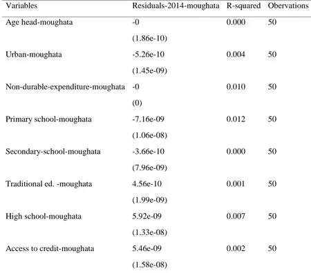
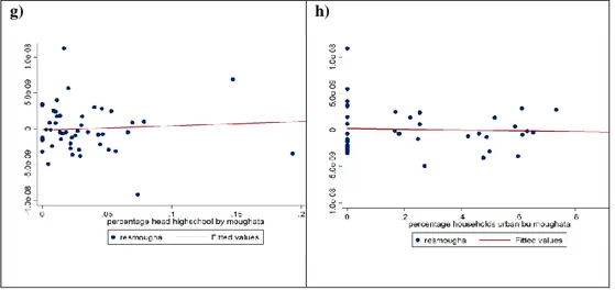
37 The variability of residuals in equation (3) is a necessary condition for the identification, but does not make the exclusion restriction bulletproof. In an effort to address this problem, we turn to data from the 2008 EPCV and show that residuals in Figure 7 are not predicted by past area and household characteristics. This is shown in Figure 8, where access to credit is considered, along with a set of other variables, over the period 2003-2008. The lack of panel data on household across the two waves (2008 and 2014) forces the analysis at the area (moughata) level. We probe empirically the validity of instrument computing the estimation (Note 18) of the average value of residuals 𝐸𝑎2014-in area-(Note 19) on the average value of the variables measured in 2008, 𝐸𝑎2008. More in details, we consider the relationship
between the residuals and a number of indicators, such as: educational indicators at different levels, the percentage of households located in urban areas, the average age of the household head, the percentage of households that had access to credit in 2008 and the average value of expenditure on non-durable goods.
The following equation is then estimated: 𝐸𝑎2014= 𝛼 +𝜌𝐸
𝑎2008+ 𝜀𝑎 (4)
Table 2 reports the results related to the estimation of equation (4) and shows that the residuals in 2014 are orthogonal to the outcomes measured in 2008. The coefficients are equal to zero or not significant. In addition, Figure 8 reports the scatterplot of these two variables, with a superimposed linear fit from the same regression. The figure offers little evidence of correlation with past characteristics, thus corroborating the exogeneity of the instrument used in the main equation.
38
Table 2. Residuals in 2014 on Outcomes in 2008- OLS Estimate
Variables Residuals-2014-moughata R-squared Obervations
Age head-moughata -0 0.000 50 (1.86e-10) Urban-moughata -5.26e-10 0.004 50 (1.45e-09) Non-durable-expenditure-moughata -0 0.010 50 (0)
Primary school-moughata -7.16e-09 0.012 50 (1.06e-08)
Secondary-school-moughata -3.66e-10 0.000 50 (7.96e-09)
Traditional ed. -moughata 4.56e-10 0.001 50 (1.99e-09)
High school-moughata 5.92e-09 0.007 50 (1.33e-08)
Access to credit-moughata 5.46e-09 0.002 50 (1.58e-08)
Note. The treatment variables are the average value of the head age, the percentage
households located in urban area; the percentage of household head educated at primay school, secondary school, traditional level and high school; the average value of non-durable expenditure; the percentage of households that have access to credit. All the variables are at moughataa level. Standard errors in parentheses.
39
a) b)
c) d)
40
g) h)
Figure 8. Residuals (2014) Compared with Outcomes (2008), Average Values by Moughata
7. Results
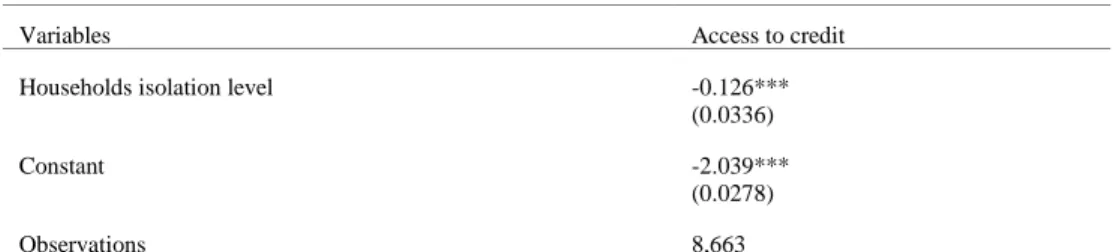
Table 3 and Table 4 provide a probit estimation of Equation 2. The analysis is clustered by moughata, and robust standard errors are reported throughout. The results show that HIL is negatively correlated with access to credit (Table 3). The coefficients are statistically significant and economically meaningful, and the results are robust to the inclusion of the household characteristics (Table 4). The age and education level of the head of household and the household’s location in an urban area have especially positive and significant effects on the probability of accessing credit. Estimates of 𝛽 are presented along with standard errors, and statistical significance at the 1, 5 and 10 percent levels is noted.
41
Table 3. Probit Estimate of HIL and Access to Credit
Variables Access to credit
Households isolation level -0.126*** (0.0336)
Constant -2.039***
(0.0278)
Observations 8,663
Note. The treatment variable is the household isolation level (HIL).Standard errors are
clustered by moughata
*** Significant at the 1 percent level. ** Significant at the 5 percent level. * Significant at the 10 percent level.
Table 4. Probit Estimate of HIL and Access to Credit
Variables Access to credit Household isolation level -0.0871***
(0.0334) Land ownership -0.0671 (0.534) Age head 0.0405*** (0.0140) Urban 0.321** (0.127) Number of males 0.0269 (0.0242) Age household -0.00169 (0.00336) Age head square -0.000359***
(0.000135) Number of kids 0.00547 (0.0382) Head female -0.0164 (0.0757) Traditional ed. -0.00707 (0.114) Primary school 0.351** (0.168) Secondary school 0.682*** (0.139) Secondary tec-prof 0.877** (0.381) High school 1.078*** (0.148) Size -0.00642 (0.0165) Constant -3.304*** (0.353) Observations 8,663
Note. The treatment variable is the household isolation level (HIL). The independent
variables are a dummy for urban location and for education level, household size, a dummy for female head of household, land ownership, number of adult males, number of children, age of household head, age of household head squared, average age of household members, and area-level fixed effects. Standard errors are clustered by moughata.
*** Significant at the 1 percent level. ** Significant at the 5 percent level. * Significant at the 10 percent level
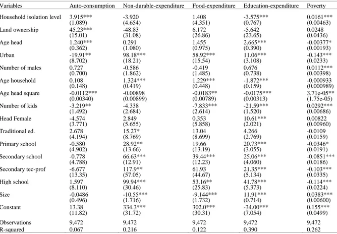
42 Table 5 and Table 6 present the reduced form (RF) estimates. They show that the HIL is positively correlated with the consumption of household production and poverty incidence and negatively correlated with education spending. These results are robust to the inclusion of all other household characteristics defined in the analysis.
Table 5. Impact of HIL on Welfare-RF Estimates
Variables Auto-consumption Non-durable-expenditure Food-expenditure Education-expenditure Poverty Household isolation level 5.799*** -14.87*** -5.181 -6.512*** 0.0308** * (0.938) (4.699) (4.067) (1,149) (0.00614) Constant 36.40*** 373.2*** 347.3*** 76.63*** 0.213*** (0.00710) (0.0356) (0.0308) (0.00870) (4.65e-05) Observations 9,472 9,472 9,472 9,472 9,472 R-squared 0.063 0.161 0.085 0.067 0.112
Note. The treatment variable is the household isolation level (HIL). Standard errors are clustered by moughata
*** Significant at the 1 percent level. ** Significant at the 5 percent level. * Significant at the 10 percent level.
Table 6. Impact of HIL on Welfare-RF Estimates
Variables Auto-consumption Non-durable-expenditure Food-expenditure Education-expenditure Poverty Household isolation level 3.915*** -3.920 1.408 -3.575*** 0.0161***
(1.089) (4.654) (4.351) (0.767) (0.00463) Land ownership 45.23*** -48.83 6.172 -5.642 0.0248 (15.01) (31.08) (26.86) (23.65) (0.0436) Age head 1.240*** 0.291 1.455 2.665*** -0.00377* (0.362) (1.080) (0.975) (0.390) (0.00193) Urban -19.91** 98.18*** 58.92*** 11.06*** -0.143*** (8.702) (18.21) (15.54) (3.108) (0.0233) Number of males 0.727 -0.586 -0.419 0.676 0.0112*** (0.700) (1.862) (1.485) (0.738) (0.00398) Age household 0.108 1.324*** 1.229*** -1.872*** -0.000933 (0.148) (0.419) (0.448) (0.159) (0.000989) Age head square -0.0112*** -0.00898 -0.0183** -0.0175*** 3.71e-05** (0.00340) (0.00899) (0.00789) (0.00313) (1.75e-05) Number of kids -3.219** -4.338 -7.833*** -21.59*** 0.0292*** (1.492) (2.684) (2.614) (1.520) (0.00686) Head Female -4.574 2.849 0.353 10.61*** 0.00822 (3.771) (5.655) (5.858) (2.021) (0.00960) Traditional ed. 2.678 15.27* 13.04 4.266 -0.0109 (4.194) (8.769) (8.699) (2.769) (0.0159) Primary school -0.580 28.92** 19.66 20.73*** -0.0346* (4.902) (13.66) (13.19) (3.055) (0.0191) Secondary school -0.778 66.63*** 39.44*** 25.06*** -0.0851*** (4.788) (12.91) (12.23) (4.060) (0.0186) Secondary tec-prof -6.677 117.9** 61.93 21.35*** -0.103*** (13.35) (57.05) (44.67) (5.134) (0.0335) High school 1.597 99.94*** 53.16** 41.78*** -0.114*** (8.110) (30.46) (25.83) (5.373) (0.0224) Size -0.0486 -10.55*** -9.144*** 11.91*** 0.0383*** (0.496) (1.716) (1.732) (0.714) (0.00600) Constant 13.38 334.3*** 302.0*** -34.00*** 0.155*** (11.82) (31.72) (30.31) (7.054) (0.0499) Observations 9,472 9,472 9,472 9,472 9,472 R-squared 0.067 0.216 0.122 0.390 0.262
43 Note. (refers to Table 6, previous page). The treatment variable is the household isolation level (HIL).
The independent variables are a dummy for urban location and for education level, household size, a dummy for female head of household, land ownership, number of adult males, number of children, age of household head, age of household head squared, average age of household members, and area-level fixed effects. Standard errors are clustered by moughata.
*** Significant at the 1 percent level. ** Significant at the 5 percent level. * Significant at the 10 percent level.
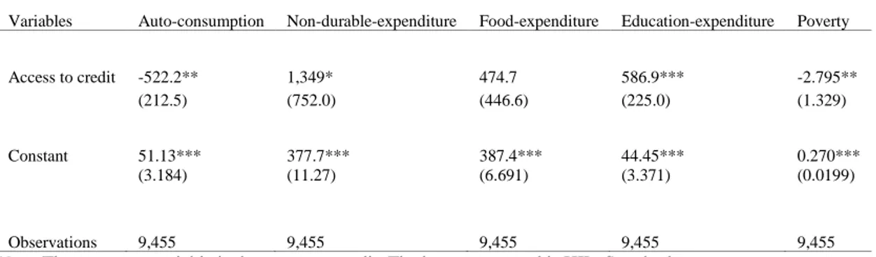
Table 7 and Table 8 present Instrumental Variable (IV) estimates of the relationship between access to credit and the key variables used in the analysis. Estimates of 𝛼 are reported along with standard errors, and statistical significance at the 5 and 10 percent levels is noted.
Table 7. Impact of Access to Credit on Welfare - Instrumental Variable (IV) Estimates
Variables Auto-consumption Non-durable-expenditure Food-expenditure Education-expenditure Poverty
Access to credit -522.2** 1,349* 474.7 586.9*** -2.795**
(212.5) (752.0) (446.6) (225.0) (1.329)
Constant 51.13*** 377.7*** 387.4*** 44.45*** 0.270***
(3.184) (11.27) (6.691) (3.371) (0.0199)
Observations 9,455 9,455 9,455 9,455 9,455
Note. The treatment variable is the access to credit. The instrument used is HIL. Standard errors are
clustered by moughata.
*** Significant at the 1 percent level. ** Significant at the 5 percent level. * Significant at the 10 percent level.
44
Table 8. Impact of Access to Credit on Welfare - IV Estimates
Variables Auto-consumption Non-durable-expenditure Food-expenditure Education-expenditure Poverty Access to credit -506.4* 524.4 -168.2 464.0** -2.116 (264.3) (725.2) (540.5) (230.7) (1.421) Land ownership 51.40** -55.12 8.301 -11.31 0.0506 (20.87) (35.15) (26.26) (29.10) (0.0500) Age head 2.608*** -1.186 1.856 1.419 0.00206 (1.011) (2.337) (1.807) (0.998) (0.00496) Urban -12.72 90.44*** 61.06*** 4.458 -0.112*** (11.16) (24.79) (20.13) (4.652) (0.0336) Number of males 1.756 -1.715 -0.121 -0.276 0.0155** (1.555) (3.177) (1.967) (1.322) (0.00710) Age household 0.0387 1.381*** 1.197*** -1.809*** -0.00121 (0.191) (0.446) (0.461) (0.182) (0.00118) Age head square -0.0228** 0.00364 -0.0217 -0.00694 -1.26e-05 (0.00901) (0.0192) (0.0150) (0.00874) (4.27e-05) Number of kids -2.514 -5.113* -7.661*** -22.28*** 0.0319*** (2.050) (2.891) (2.868) (1.975) (0.00881) Head female -6.306 4.525 -0.329 12.05*** 0.00117 (5.264) (6.982) (5.831) (3.978) (0.0178) Traditional ed. -0.826 19.00* 11.94 7.399 -0.0258 (6.471) (10.36) (8.975) (5.114) (0.0238) Primary school 9.074 19.36 23.18 11.74 0.00554 (9.644) (20.88) (18.31) (7.987) (0.0432) Secondary school 34.19* 30.52 51.15 -7.154 0.0613 (20.11) (54.55) (41.67) (18.79) (0.108) Secondary tec-prof 48.00 61.21 80.14 -28.89 0.125 (54.49) (110.8) (85.59) (46.78) (0.248) High school 87.59** 10.85 82.01 -36.62 0.244 (44.39) (123.2) (95.78) (37.26) (0.238) Size -0.437 -10.14*** -9.256*** 12.28*** 0.0367*** (0.806) (2.169) (1.721) (0.864) (0.00766) Constant -13.80 443.7*** 376.4*** -22.14 -0.0386 (24.45) (53.02) (45.73) (22.29) (0.103) Observations 9,455 9,455 9,455 9,455 9,455
Note. The treatment variable is the access to credit. The instrument used is HIL. The independent
variables are a dummy for urban location and for education level, household size, a dummy for female head of household, land ownership, number of adult males, number of children, age of household head, age of household head squared, average age of household members, and area-level fixed effects. Standard errors are clustered by moughata.
*** Significant at the 1 percent level. ** Significant at the 5 percent level. * Significant at the 10 percent level.