U
NIVERSITÀ
D
ELLA
C
ALABRIA
Dipartimento di Meccanica
D
OTTORATOD
IR
ICERCA INI
NGEGNERIAM
ECCANICACICLO XXV (2009-2012)
SCUOLA DI DOTTORATO “PITAGORA” IN SCIENZE INGEGNERISTICHE
SSD:
ING-IND/15
-
D
ISEGNO EM
ETODI DELL’I
NGEGNERIAI
NDUSTRIALEInnovative methodologies
for multi-view 3D reconstruction
of Cultural Heritage
A DISSERTATION SUBMITTED IN PARTIAL FULFILMENT OF THE REQUIREMENTS FOR THE
DOCTORAL RESEARCH DEGREE IN MECHANICAL ENGINEERING
Doctoral Research Director
Supervisor
Prof. Sergio Rizzuti
Prof. Fabio Bruno
Candidate
Ing. Alessandro Gallo
ii
Abstract
This dissertation focuses on the use of multi-view 3D reconstruction techniques in the field of cultural heritage. To name just a few applications, a digital 3D acquisition can be used for documentation purposes in the event of destruction or damage of an artefact, or for the creation of museums and virtual tourism, education, structural studies, restoration, etc... All these applications require high precision and accuracy to reproduce the details, but there are other important characteristics such as low cost, ease of use, the level of knowledge needed to operate the systems, which have also to be taken into account. At the present time, the interest is growing around the use of images for the digital documentation of cultural heritage, because it is possible to obtain a 3D model by the means of common photographic equipment. In this work, we have investigated multi-view 3D reconstruction techniques in two specific fields that have not been treated in literature: the 3D reconstruction of small objects (from few mm to few cm) and the survey of submerged archaeological finds.
As for the 3D reconstruction of small objects, a new methodology based on multi-view and image fusion techniques has been developed. The used approach solves the problems related to the use of macro lenses in photogrammetry, such as the very small depth of field and the loss of quality due to diffraction. Since image matching algorithms cannot work on blurred areas, each image of the sequence is obtained by merging pictures acquired at different focus planes. The methodology has been applied on different case studies, and the results have shown that it is possible to reconstruct small complex objects with a resolution of 20 microns and an accuracy of 10 microns. For which concerns the underwater imaging, a preliminary comparative study between active and passive techniques in turbid water has been conducted. The experimental setup consists in a 3D scanner designed for underwater survey, composed by two cameras and a projector. An analysis on the influence of the colour channel has been conducted, showing how it is possible to obtain a cleaner reconstruction by using the green channel only. The results have shown a denser point cloud when using the passive technique, characterized by missing areas since the technique is more sensible to
iii turbidity. By contrast, the reconstruction conducted with the active technique have shown more stable results as the turbidity increases, but a greater noise.
A multi-view passive technique has been experimented for the survey of a submerged structure located at a depth of 5 meters, on a seabed characterized by poor visibility conditions and the presence of marine flora and fauna.
We performed an analysis of the performances of a multi-view technique commonly used in air in the first instance, highlighting the limits of the current techniques in underwater environment. In such conditions, in fact, it has not been possible to obtain a complete reconstruction of the scene. The second stage of the process was the testing of image enhancement algorithms in order to improve matching performances in poor visibility conditions. In particular, a variational analysis of the factors that influence the quality of the 3D reconstruction, such as the image resolution and the colour channel, has been performed. For this purpose, the data related to the parameters of interest, such as the number of features extracted or the number of oriented cameras, have been evaluated. The statistical analysis has allowed to find the best combination of factors for a complete and accurate 3D reconstruction of the submerged scenario.
iv
Sommario
La presente tesi tratta l’impiego di tecniche di ricostruzione 3D multi-vista nell’ambito dei beni culturali. Un’acquisizione digitale 3D trova impiego nella documentazione in caso di distruzione o danneggiamenti di un manufatto, nella creazione di musei e turismo virtuale, educazione, analisi strutturale, pianificazione di interventi di restauro, ecc... Queste applicazioni richiedono un’alta precisione e accuratezza per riprodurre tutti i dettagli dell’oggetto, ma altri importanti requisiti di cui si deve tenere conto sono rappresentati dal costo, semplicità di utilizzo e dal grado di specializzazione richiesto Attualmente, vi è un crescente interesse per l’utilizzo di immagini digitali per la documentazione del patrimonio culturale, in quanto rendono possibile la generazione di contenuti 3D mediante l’utilizzo di comuni apparecchiature fotografiche. Nel presente lavoro sono state studiate tecniche di ricostruzione 3D multi-vista in due ambiti specifici che attualmente non sono stati sufficientemente trattati in letteratura: la ricostruzione 3D mediante tecniche passive di piccoli oggetti (da pochi mm a pochi cm) ed il rilievo di reperti archeologici sommersi.
Nell’ambito della ricostruzione di piccoli oggetti, è stata sviluppata una nuova metodologia basata su tecniche multi-vista e di image fusion. L’approccio utilizzato risolve i problemi che si riscontrano nell’utilizzo di ottiche macro in fotogrammetria, quali la ridotta profondità di campo e la perdita di nitidezza dovuta alla diffrazione. Dal momento che gli algoritmi di image matching non lavorano al meglio se sono presenti aree sfocate, ogni immagine della sequenza è il risultato della fusione di più immagini riprese a diverse profondità di campo. La metodologia è stata applicata su differenti casi studio, e i risultati ottenuti hanno dimostrato che è possibile ricostruire oggetti complessi con una risoluzione di 20 micron e un’accuratezza di circa 10 micron.
Nell’ambito dell’imaging subacqueo, è stato condotto un confronto preliminare tra tecniche attive e passive in condizioni di acqua torbida. Il setup sperimentale si basa su di uno scanner 3D progettato per il rilievo subacqueo composto da due fotocamere ed un proiettore. È stata condotta un’analisi sull’influenza del canale colore, che ha mostrato come sia possibile ottenere ricostruzioni più pulite utilizzando il solo canale verde. I risultati mostrano una maggior densità della nuvola di punti ricostruita mediante
v la tecnica passiva, che è caratterizzata però da aree mancanti data la maggior sensibilità alla torbidità. Di contro, le ricostruzioni effettuate con la tecnica attiva presentano una maggior stabilità all’aumentare della torbidità ma un rumore maggiore.
Una tecnica passiva multi-vista è stata sperimentata per il rilievo di una struttura sommersa rinvenuta ad una profondità di 5 metri su un fondale caratterizzato da condizioni di scarsa visibilità e presenza di flora e fauna acquatica. Una prima fase ha previsto l’analisi delle prestazioni di una tecnica multi-vista largamente utilizzata in aria, evidenziando i limiti delle attuali tecniche in ambito subacqueo. In tali condizioni, infatti, non è stato possibile ottenere una ricostruzione completa della scena. Una seconda fase ha previsto la sperimentazione di algoritmi di image enhancement al fine di migliorare le prestazioni degli algoritmi di matching in condizioni di scarsa visibilità. In particolare è stata utilizzata un’analisi variazionale dei fattori che hanno una certa influenza sulla qualità della ricostruzione 3D, quali ad esempio la risoluzione delle immagini ed il canale colore. A tal fine sono stati valutati i dati relativi ad opportuni parametri di interesse, quali il numero di features estratte o il numero di camere orientate. L’analisi statistica ha consentito di trovare la combinazione di fattori ottimale per una completa ed accurata ricostruzione 3D dello scenario sommerso.
vi
Acknowledgments
The research presented in this work would not have been possible without the invaluable guide and support of the following people:
my supervisor Prof. Fabio Bruno for the constant assistance and encouragement during my work;
the Prof. Maurizio Muzzupappa and the other members of my research team; the Prof. Sergio Rizzuti, Doctoral Research Director;
my colleagues with whom I constantly shared knowledge and experience;
the head of the Centre of Machine Perception (CMP) in Prague, Prof. Vaclav Hlavac and the Prof. Radim Šára for the interesting study experience during the doctoral stage; the technicians of Laboratory of the Department of Mechanics at the University of Calabria;
vii
List of Figures
Figure 1.1. Image formation pipeline: representation of various sources of noise and the typical digital
post-processing steps. ... 7
Figure 1.2. Bayer pattern (a) and demosaicing procedure (b). ... 11
Figure 1.3. The Foveon sensor. ... 12
Figure 1.4. Pinhole camera model. ... 13
Figure 1.5. For every pixel m, the corresponding pixel in the second image m’ must lie somewhere along a line l’. This property is referred to as the epipolar constraint. See the text for details. ... 15
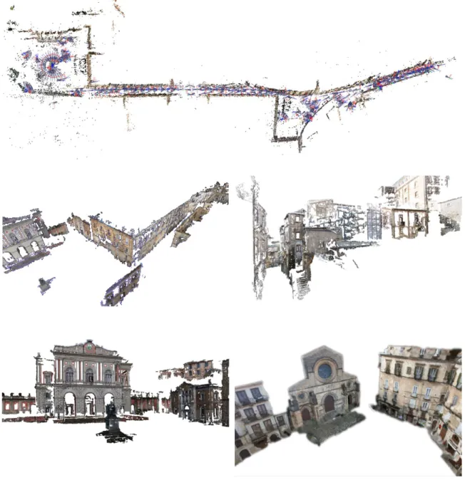
Figure 1.6. Survey of the historical centre of Cosenza (Italy): aerial view of the reconstructed area including camera positions (top) and 3D pointy clouds related to relevant points of interest... 22
Figure 1.7. 3D point cloud of the Certosa of Serra San Bruno (Italy), destroyed in 1783 by a terrible earthquake. ... 23
Figure 1.8. Triangulated surface (a) and textured 3D model (b) of the B. Telesio Statue located in Cosenza (Italy). ... 23
Figure 1.9. Triangulated surface (a) and textured 3D model (b) of a wooden statue of Virgin Mary. ... 24
Figure 1.10. Triangulated surface (a) and textured 3D model (b) of a bronze archaeological find. ... 25
Figure 1.11. Triangulated surface (a) and textured 3D model (b) of a bas-relief with dimensions of 50 x 50 cm. ... 25
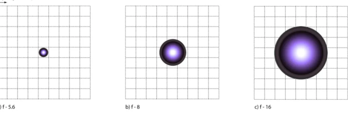
Figure 2.1. Size of the Airy disk at increasing f-numbers relative to the pixel dimension of a Nikon D5000 digital reflex camera. ... 33
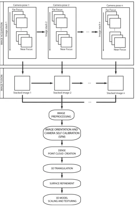
Figure 2.2. Pipeline of the implemented methodology for the acquisition and 3D reconstruction of small sized objects. ... 35
Figure 2.3. Example of three images acquired at different focus distances and the staked image resulting from the fusion of 22 slices. ... 37
Figure 2.4. Effect of diffraction due to the use of a very small aperture. The image resulting from the fusion of 22 slices taken at different focus distance with the aperture set to f-11, is compared to the one taken at f-64, highlighting the loss of sharpness. ... 38
Figure 2.5. Experimental setup. A Nikon D5000 reflex camera equipped with a Tamron 90 mm macro lens and the rotational stage, fixed on an optical table. Some led lamps ensure proper lighting... 40
Figure 2.6. White support plate used to scale the final model and to help the image pre-processing (masking and white balance). ... 41
Figure 2.7. Two certified gauge blocks are placed on a rectified surface and mounted on the rotational stage in order to verify the accuracy. ... 42
Figure 2.8. Sample image enhanced by using the Wallis filter (right) compared to the original uncorrected image (left). ... 42
viii
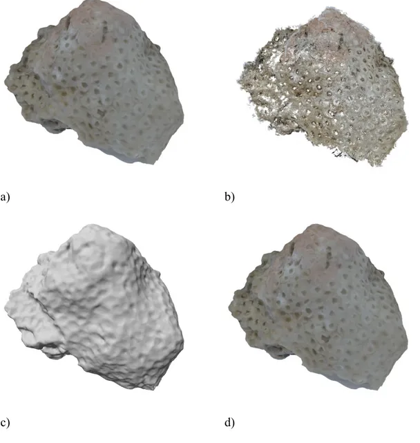
Figure 2.9. System resolution and accuracy evaluation: the reconstructed 3D model (a) has been compared to the relative CAD model (b). ... 43 Figure 2.10. Fist case study, a bronze zoomorphic fibula with dimensions (LxWxH) of 37x18x16 mm. . 45 Figure 2.11. Second case study. Four specimens of encrustations, (a) T2, (b) T9 (c) T10 and (d) T16, extracted from a marble statue of a bearded Triton. The support plate is a square of 25 x 25 mm. 46 Figure 2.12. Third case study. A calcareous sample (left) and a marble sample (right). The support plate is a square of 25x25mm... 47 Figure 2.13. First case study: one of the input image (a), the 3D point cloud (b), the reconstructed
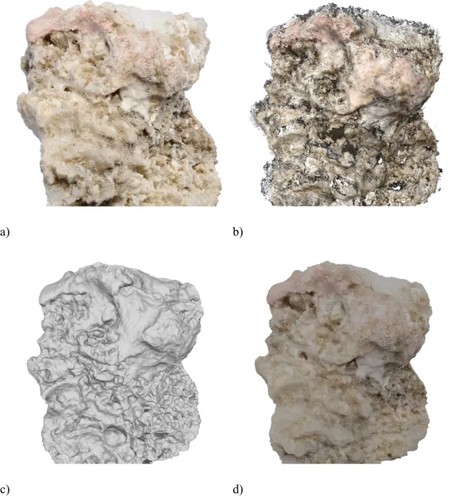
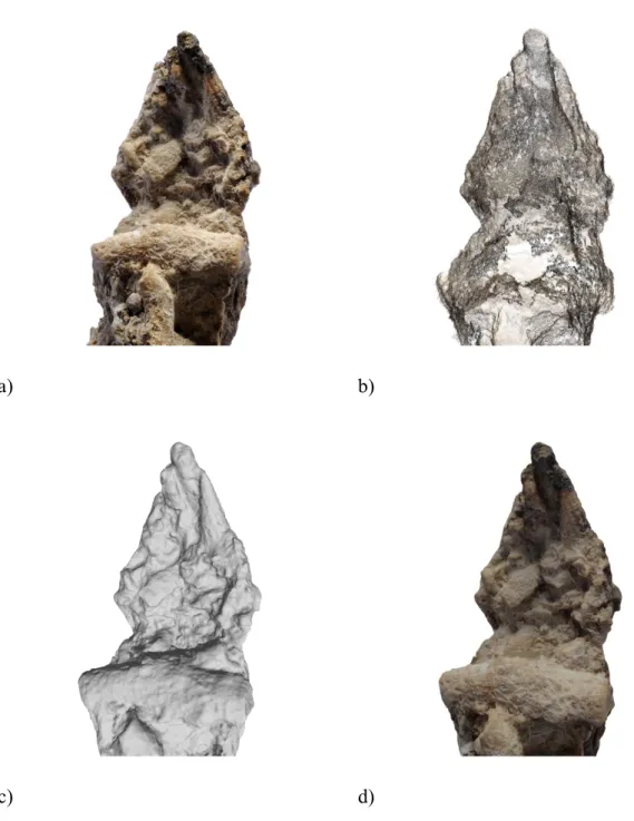
polygonal mesh (c) and the final textured 3D model (d). ... 49 Figure 2.14. First case study. Detail of the tail and wings. ... 49 Figure 2.15. Second case study, T2 specimen: one of the input image (a), the 3D point cloud (b), the reconstructed polygonal mesh (c) and the final textured 3D model (d). ... 50 Figure 2.16. Second case study, T9 specimen: one of the input image (a), the 3D point cloud (b), the reconstructed polygonal mesh (c) and the final textured 3D model (d). ... 51 Figure 2.17. Second case study, T10 specimen: one of the input image (a), the 3D point cloud (b), the
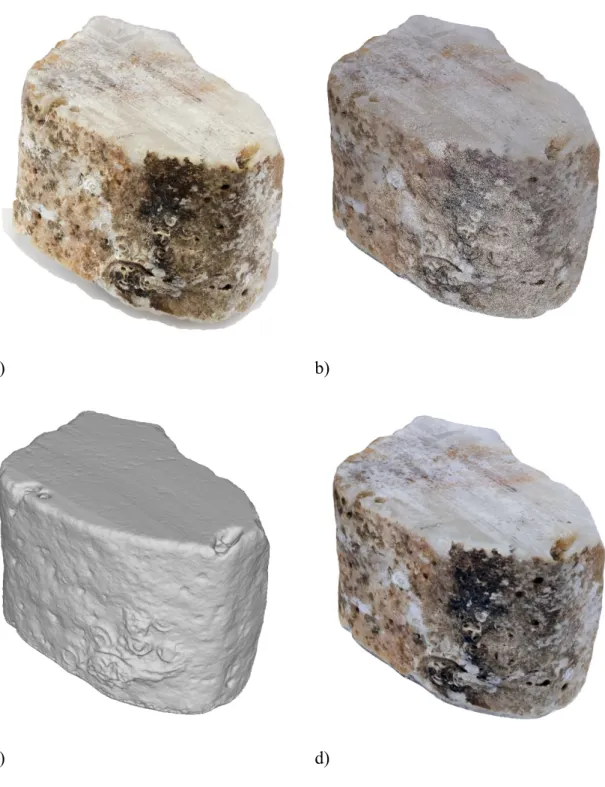
reconstructed polygonal mesh (c) and the final textured 3D model (d). ... 52 Figure 2.18. Second case study, T16 specimen: one of the input image (a), the 3D point cloud (b), the reconstructed polygonal mesh (c) and the final textured 3D model (d). ... 53 Figure 2.19. Detail of pitting on the T9 specimen (a) and gastropod in the T16 specimen. The holes due to pitting measure about 0.4 mm while the gastropod is about 4 mm long. ... 54 Figure 2.20. Third case study, M1 specimen: one of the input image (a), the 3D point cloud (b), the
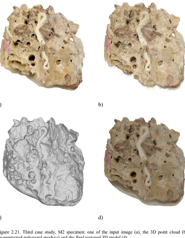
reconstructed polygonal mesh (c) and the final textured 3D model (d). ... 55 Figure 2.21. Third case study, M2 specimen: one of the input image (a), the 3D point cloud (b), the
reconstructed polygonal mesh (c) and the final textured 3D model (d). ... 56 Figure 2.22. Third case study, details of serpulids on M1 (a) and M2 (b) specimen. The mean diameter of the serpulidae on specimen M2 measures about 1 mm, while from the traces on specimen M1 the diameter of the serpulids range from 0.1 to 0.5 mm. ... 57 Figure 2.23. Comparison between the 3D reconstructions obtained by our approach for the specimens T2 (a), T9 (c) and T16 (d) and the one obtained using the multi-view stereo technique on a sequence of images taken at an aperture value of f-64 (b), (d) and (f). The diffraction effect causes a loss of detail that result in a smoother surface. ... 59 Figure 2.24. Comparison between the 3D reconstruction obtained by our approach for the specimen M1 (a) and M2 (c) and the one obtained using a sequence of images taken at the maximum f-number (b) and (d). The diffraction effect causes a loss of detail that result in a smoother surface. ... 59 Figure 2.25. Comparison between the 3D reconstruction obtained by our approach for the specimens T2 (a) and T16 (d) and the one obtained using a depth from focus algorithm on a stack of 14 images taken at f-11 (b) and (e) and on a stack of 70 images taken at the smallest aperture of f-5.6 (c) and
ix
(f). The depth resolution relative to the depth from focus algorithm is equal to half DoF, 0.5 mm
and 0.25 mm respectively, against a resolution of 20 micrometer of our approach. ... 61
Figure 2.26. Comparison between the 3D reconstruction obtained by our approach for the specimens M1 (a) and the one obtained using a depth from focus algorithm on a stack of 86 images taken at f-4.5 (b). The depth resolution relative to the depth from focus algorithm is equal 0.25 mm, against a resolution of 20 micrometer of our approach. ... 61
Figure 3.1. On the left, triangulation of a stereo configuration composed by two cameras and a projector. The points mL and mR in left and right images respectively, are the projection on the image planes IL and IR of the same 3D point w of the object. On the right, examples of binary patterns and code shifting. ... 69
Figure 3.2. Optical setup of the underwater 3D acquisition system: underwater calibration (left) and acquisition (right). ... 71
Figure 3.3. Optical setup of the underwater 3D system. ... 72
Figure 3.4. Images of the two objects with a projected gray-code pattern, acquired at different turbidity levels. ... 73
Figure 3.5. Complete distortion model (radial plus tangential distortions) in air and clear water. The cross and the circle indicate the image centre and the principal point respectively. The contours represent the optical distortions values (in pixel). ... 75
Figure 3.6. Distribution of the re-projection error (in pixel) in air and clear water (RGB images). ... 75
Figure 3.7. Point cloud cleaning procedure. Outlier point manual selection a), selected outlier points (b), cleaned point cloud after outlier deletion (c) and final point cloud after noise filtering (d). ... 79
Figure 3.8. Point clouds obtained in different environment condition for both active and passive technique. ... 81
Figure 3.9. Acquired images and unclean point clouds at a light turbidity level (T1) in each colour channel: the blue points are due to scattering effect, highly reduced in green channel. ... 81
Figure 4.1. Geographical localization of underwater archaeological site of Baia (Italy). ... 89
Figure 4.2. Calibration panel used to manually correct the white balance. ... 91
Figure 4.3. Image acquisition using a standard aerial photography layout (a) and using oblique photographs (b)... 92
Figure 4.4 Results of the camera orientation process on original uncorrected pictures: due to the presence of a low contrasted sandy seabed, the whole scene has been reconstructed in two separated blocks relative to the North part (up, 384 pictures) and to the South part (down, 116 pictures). ... 94
Figure 4.5. Reconstructed point cloud of the North area. ... 95
Figure 4.6. Reconstructed point cloud of the South area. ... 95
Figure 4.7. Reconstructed surface and textured model of the North area. ... 96
Figure 4.8. Reconstructed surface and textured model of the South area. ... 97
Figure 5.1. A sample image enhanced with the ACE method (b), HIST method (c) and PCA method (d) compared to the original image (a). ... 103
x
Figure 5.2. Pipeline of the implemented methodology for the reconstruction of submerged scenes. ... 104 Figure 5.3. Sample images related to image set 1 (a), image set 2 (b), image set 3 (c), image set 4 (d), image set 5 (e), image set 6 (f) and image set 7 (g)... 108 Figure 5.4. Example of an anova table related to the parameter “mean extracted features”. ... 112 Figure 5.5. Graphs obtained with the multicompare function of the factors image enhancement method (a) and image pyramid level (b) related to the parameter “Mean number of extracted features”. ... 113 Figure 5.6. Example of the histogram representing the data related to the mean number of extracted
features. ... 115 Figure 5.7. Anova table relative to the parameter “mean extracted features”. ... 116 Figure 5.8. Mean number of extracted features: detailed comparison related to all the configurations. .. 117 Figure 5.9. Mean values and confidence intervals related to the parameter mean number of extracted
features... 118
Figure 5.10. Anova table related to the parameter “mean extracted features” measured on images belonging to the second image set. ... 119 Figure 5.11. Mean values and confidence intervals related to the parameter mean number of extracted
features of the second image set... 119
Figure 5.12. Anova table relative to the parameter “percentage of matched features”. ... 120 Figure 5.13. Mean values and confidence intervals related to the parameter percentage of matched
features. ... 121 Figure 5.14. Percentage of matched features: detailed comparison related to all the configurations. ... 122 Figure 5.15. Anova table related to the parameter “percentage of oriented cameras”... 123 Figure 5.16. Mean values and confidence intervals related to the parameter percentage of oriented
cameras. ... 124 Figure 5.17. Anova table related to the parameter “percentage of oriented cameras” computed from the data related to the RGB images only, which include the single component extracted by PCA correction. ... 125 Figure 5.18. Mean values and confidence intervals related to the parameter percentage of oriented
cameras, computed from the data related to only the RGB images which include the single
component from PCA correction. ... 125 Figure 5.19. Percentage of oriented cameras: detailed comparison related to all the configurations. ... 126 Figure 5.20. Anova table related to the parameter “bundle adjustment mean reprojection error”. ... 127 Figure 5.21. Mean values and confidence intervals related to the parameter bundle adjustment mean
reprojection error. ... 128
Figure 5.22. Bundle adjustment mean reprojection error: detailed comparison related to all the configurations. ... 129 Figure 5.23. Mean values and confidence intervals related to the parameter mean number of extracted
features: the analysis has been performed on images acquired using custom white balance
xi
Figure 5.24. Performances comparison of the image enhancement methods for each measured parameter. The performances of the HIST, ACE and PCA image enhancement algorithms, are compared to a
reference value related to the original images (OR). ... 132
Figure 5.25. Performances comparison of the image resolution (image pyramid) for each measured parameter. The performances of the first pyramid (High res – images resized to 50%), the second pyramid (Med res – images resized to 25%) and the third pyramid (Low res – images resized to 6.25%), are compared taking as reference the value related to the low resolution images. ... 132
Figure 5.26. Performances comparison of the colour channels for each measured parameter. The performances of the R, G and B components, are compared taking as reference the value related to the RGB images... 133
Figure 5.27. Results of the camera orientation process (enhanced pictures with HIST method): sparse point cloud and 533 oriented pictures. ... 133
Figure 5.28. Reconstructed dense point cloud. ... 134
Figure 5.29. Reconstructed surface. ... 134
Figure 5.30. Final textured 3D model - a. ... 137
xii
List of Tables
Table 2.1. The three samples prepared arranging in pair three certified gauge blocks. ... 41 Table 2.2. mean values of the extracted SIFT features for the datasets relative to the tree specimens,
reconstructed using the original images and the one enhanced by using the Wallis filter. ... 43 Table 2.3. System accuracy evaluation. The experimental results show that the system is capable to resolve up to a 20 µm step with an accuracy of about 10 microns. ... 44 Table 2.4. Results of the 3D reconstruction relative to the three case studies ... 57 Table 2.5. Time required to complete the whole 3D reconstruction pipeline. Most of the time is needed for the image acquisition phase. ... 58 Table 3.1.Measurements of the turbidity conditions. ... 70 Table 3.2. Intrinsic parameters (mean values for left and right camera) in air and water (RGB images)... 74 Table 3.3. Accuracy evaluation on a planar and cylindrical sample in air and water. ... 78 Table 3.4. Acquired 3D points per 100 pixel (Np for passive and Na for active stereo) and percentage
values of deleted 3D points (Npc% for passive Nac% for active stereo) for Amphora and Aeolus. .. 79 Table 3.5. Percentage values of deleted 3D points for active stereo technique in each colour channel, red
(Nac%-R), green (Nac%-G) and blue (Nac%-B), compared respect the values computed from RGB images (Nac%-RGB). The table is related to the object Amphora... 82 Table 3.6. Geometrical error (mean µ and standard deviation σ) calculated for active technique in the green channel: the point clouds are compared respect to a reference (Ref.). ... 82 Table 3.7. Geometrical error (mean µ and standard deviation σ) calculated for passive technique in the green channel: the point clouds are compared respect to a reference (Ref.). ... 83 Table 5.1. Influence factors and related levels used to perform the analysis of variance. ... 106
Contents
Abstract ... ii
Sommario... iv
Acknowledgments ... vi
List of Figures ... vii
List of Tables ... xii
Introduction ... 1
Thesis objectives... 4
Structure of the thesis ... 5
1. Image formation and 3D reconstruction from multiple views ... 6
1.1. Image formation ... 6
1.1.1. The digital camera ... 6
1.1.2. Colour filter arrays and demosaicing... 10
1.2. Geometry of image formation and multi-view Geometry... 12
1.2.1. Pinhole Camera Model ... 12
1.2.2. Epipolar Geometry ... 15
1.2.3. Projective Reconstruction and Self-Calibration ... 16
1.3. Multi-view 3D Reconstruction ... 16
1.3.1. Camera calibration ... 17
1.3.2. Structure from motion ... 18
1.3.3. Multi view stereo ... 19
1.4. Experimentation of a multi-view stereo algorithm in real case studies ... 21
1.4.1. Large scale scenes ... 21
1.4.2. Monuments and statues ... 23
2. Multi-view 3D reconstruction of small sized objects ... 26
2.1. Introduction ... 26
2.2. Related works... 28
2.3.1. Macro photography... 29
2.3.2. Image fusion techniques for extended Depth of Field ... 30
2.3.3. Depth from focus ... 31
2.3.4. Multi-view photogrammetric reconstruction ... 31
2.3.5. Problems in macro photogrammetry ... 32
2.4. The proposed methodology for small object reconstruction... 34
2.4.1. Image acquisition ... 34
2.4.2. Determination of shooting parameters ... 34
2.4.3. Image stack acquisition ... 36
2.4.4. Image fusion and pre-processing ... 36
2.4.5. Multi-view 3D reconstruction ... 37
2.4.6. Triangulation ... 39
2.4.7. Surface refinement ... 39
2.4.8. Scaling and texturing ... 39
2.5. Experimental setup... 40
2.6. Accuracy evaluation... 41
2.7. Experimentation ... 44
2.7.1. Description of the case studies ... 44
2.7.2. Image acquisition ... 47
2.7.3. 3D reconstruction ... 48
2.7.4. Experimental results ... 48
2.8. Comparison with depth from focus technique ... 60
2.9. Summary and discussion... 62
3. Comparative analysis between active and passive stereo techniques for underwater 3d modelling of close-range objects ... 64
3.1. Introduction ... 64
3.2. Related works... 65
3.2.1. Optical imaging systems ... 65
3.2.2. Camera calibration in underwater environment ... 66
3.3. Active and passive stereo techniques ... 67
3.3.1. 3D stereo reconstruction ... 67
3.4. Experimentation ... 69
3.4.1. Underwater setup ... 71
3.4.2. Calibration ... 74
3.4.3. 3D reconstruction - Passive stereo... 76
3.4.4. 3D reconstruction - Active stereo ... 77
3.4.5. Accuracy evaluation ... 77
3.5. Results analysis ... 77
3.5.1. Point cloud editing ... 78
3.5.2. 3D points density ... 78
3.5.3. Multi-channel analysis ... 80
3.5.4. Geometrical error ... 82
3.6. Discussion ... 83
3.7. Concluding Remarks ... 84
4. Experimentation of multi-view 3D reconstruction techniques in underwater environment ... 85 4.1. Introduction ... 85 4.2. Related works... 86 4.3. Archaeological context ... 88 4.4. Experimentation ... 89 4.4.1. Experimental setup ... 90 4.4.2. Image acquisition ... 90 4.4.3. Multi-view 3D reconstruction ... 93 4.5. Conclusions ... 98
5. Underwater image pre-processing algorithms for the improvement of multi-view 3D reconstruction ... 99
5.1. Introduction ... 99
5.2. State of the art of underwater image pre-processing algorithms ... 101
5.3. Colour enhancement of underwater images ... 102
5.4. Description of the adopted methodology ... 104
5.4.1. Design of the experimental campaign ... 104
5.4.2. Datasets generation ... 110
5.5.1. Anova analysis ... 111
5.5.2. Mean extracted features ... 114
5.5.3. Percentage of matched features ... 119
5.5.4. Percentage of oriented cameras ... 123
5.5.5. Bundle adjustment mean reprojection error ... 127
5.5.6. Effects of white balance correction ... 128
5.5.7. Discussion ... 130
5.6. Results ... 133
5.7. Conclusions ... 136
Conclusions ... 139
1
Introduction
3D modelling is defined as the process that starts with the acquisition of metric data and ends with the creation of a 3D virtual model with which is possible to interact on a computer. Usually the term is used to denote the transition from a point cloud to a continuous surface, which is actually only one of the steps of a more complex process. The modelling of 3D objects and scenes is nowadays a topic of great interest not only in industry, robotics, navigation and body scanning, but also in the field of Cultural Heritage. A digital 3D acquisition can be used for documentation in the event of destruction or damage of an artifact, the creation of museums and virtual tourism, education, structural studies, restoration, etc... All these applications require high precision and accuracy to reproduce the details, but there are other important characteristics such as low cost, ease of handling, the level of automation in the process, which have also to be taken into account.
Digital models are nowadays employed everywhere, widely diffused through the Internet and handled on low-cost computers and smartphones. Even if the creation of a simple 3D model seems an easy task, a considerable effort is still required to get a precise model of a complex object, painted with a high resolution texture.
Generally speaking, the three-dimensional object measurement techniques can be classified into contact methods, such as CMM (coordinate measuring machines), and
non-contact methods, such as laser scanning and photogrammetry.
There are different approaches that can be used for the generation of a 3D model using non-contact systems, which can be grouped in active and passive techniques in relation to the type of sensor employed.
Regarding both active and passive techniques, the methods used to build a 3D model from digital images can be classified in:
1) Image-based rendering. This method creates new views of a 3D scene directly from the images (Shum & Kang 2000), and for this purpose it is necessary to know the camera positions. Alternatively it is possible to compute the camera motion from a sequence of very small baseline images.
2 2) Image-based modelling. The image based methods use passive sensors (still or video cameras) to acquire images from which 3D information can be extracted. This method is widely used for city modelling (Grün 2000) and architectural object reconstruction (El-Hakim 2002), and may be implemented with simple and low-cost hardware. Although the best results can be obtained when user interaction is involved, the image-based modelling methods retrieve the 3D coordinates of a pixel by solving the correspondence problem or using shape-form-x approaches, such as shape from stereo, shape from shading and shape from silhouette methods.
3) Range-based modelling. This method requires specialized and expensive hardware, commonly known as 3D scanners, but directly provides the 3D data of the object in the form of a point cloud. Usually this system does not provide colour information, but recent laser scanners integrate a colour camera mounted in a fixed and known position relative to the scanner reference system. However, in order to obtain the best results in terms of surface texture, it is necessary to use separated still cameras (Beraldin et al. 2002; Guidi et al. 2003). 3D scanners can be used on different scales, from tens of meters (e.g.: buildings, monuments, etc.) to few centimetres (e.g.: coins, pottery, etc.), and often require multiple scans that will be aligned to cover the whole object surface.
4) Combination of both image-based and range-based modelling. In some cases, such as the reconstruction of large architectural places, the use of just one of the two methods is not sufficient to describe the geometrical information of the object, so the use of a technique integrating range-based and image-based methods is necessary (El-Hakim & Beraldin 1995).
After the measurements, a polygonal surface has been created in order to build a realistic representation of the object. Then, the model can be mapped with a high quality texture to allow a photo-realistic visualization, necessary for immersive visualization and interaction.
This thesis will focus on image-based modelling, with special attention on passive imaging methods used to acquire 3D information from multiple views in the context of Cultural Heritage.
3 At the present time, there is an increasing interest in the use of images for the digital documentation of cultural heritage (Zubrow 2006). Their high flexibility, reduced cost and low level of knowledge required to inexperienced users, make the use of images the best choice for the 3D survey of individual artefacts or complex archaeological sites, although the usability of the raw data produced is non-straightforward and some post-processing becomes necessary.
Several new tools that can be used to obtain three-dimensional information from unorganized image collections are now available for the public and used for survey. Both COTS and open source solutions based on dense stereo matching are available, giving the possibility to generate 3D content without the need of high-cost hardware, just by using a simple still camera.
The commercial software PhotoScan (Agisoft LCC. 2010) has demonstrated to be an effective tool for 3D content development from overlapping images (Verhoeven 2011), making the reconstruction very straightforward, since the process is almost automatic and consist in a simple three-step procedure (image alignment, 3D model creation, texturing).
The use of open source 3D modelling solutions is becoming increasingly popular in the documentation of Cultural Heritage. The workflow based on Bundler (Snavely et al. 2007) for camera network orientation and PMVS2 (Furukawa & Ponce 2007) for dense reconstruction is one of the most widely used. These tools do not require taking care during acquisition, since the process can be successfully applied on unordered image collections or on pictures taken from the Internet (Agarwal et al. 2009). Moreover, the image orientation stage is carried out without user interaction and there is no need to use markers, which were usually employed in the standard photogrammetric survey. However, the “freedom” of these tools may affect the quality and reliability of the survey by reducing the possibility to use their output as a metric model, making them fit for visualization purposes only. With a more careful planning of the acquisition phase and with a little effort in the post-processing stage, these methods can be used for accurate 3D survey.
In the field of Cultural Heritage these 3D modelling solutions have been successfully applied in different works. In (Dellepiane et al. 2012) a methodology based on the use
4 of open source dense stereo matching systems has been presented. It has been applied on the monitoring of the archaeological excavation at the archaeological site of Uppàkra. In (Barazzetti et al. 2011) low cost software has been used to reconstruct the “G1” temple in MySon, Vietnam, which was listed as a UNESCO World Cultural Heritage site, demonstrating the effectiveness and accuracy of the methodology.
Image-based 3D modelling techniques represent a valid alterative to more specialized and expensive equipment and many research areas and applications still have to be explored in depth.
The research presented in this thesis focuses on two specific areas that, at the present, have not yet been adequately addressed: the 3D reconstruction of small objects and the survey of submerged structures in turbid underwater environment. Specific methodologies and tools have been developed to increase the performances of multi-view 3D reconstruction algorithms in these two challenging fields.
Thesis objectives
The main objective of this thesis is the study and the application of passive multi-view stereo techniques for Cultural Heritage purposes, aiming to satisfy the following needs:
• Developing a methodology and an experimental setup for the acquisitions of small sized objects;
• Testing the performances of the combination of a passive multi-view stereo technique and an image fusion method for the 3D reconstruction of small sized objects;
• Comparing two whole-field (active and passive) techniques for 3D underwater acquisition;
• Understanding the performances of image enhancement algorithms for acquisitions in underwater environment;
• Experimentation of a multi-view stereo technique for the 3D reconstruction of submerged structures in high turbidity conditions.
5
Structure of the thesis
Chapter 1 presents the background about the image formation in digital cameras and 3D reconstruction from multiple views.
Chapter 2 presents a new methodology for the 3D reconstruction of small sized objects (from few millimetres to few centimetres) using a multi-view stereo algorithm on a sequence of images acquired with a macro lens. Each image of the sequence is obtained with an image fusion technique that merges a stack of pictures acquired at different focus planes to extend the small depth of field at high magnification.
A comparison between an active stereo technique and a passive stereo technique in underwater environment is discussed in Chapter 3. The experimental tests on medium-sized objects have been conducted in a water tank to control the turbidity.
Chapter 4 describes the survey conducted at the underwater archaeological site of Baiae (Naples, Italy), characterized by a poor visibility due to turbidity. This condition negatively affects the 3D reconstruction, preventing to create a complete model of the site.
Chapter 5 presents the methodology developed for the 3D reconstructions in underwater environment. This is based on the use of image enhancement methods to improve the performance of a multi-view stereo technique. The statistical approach used to test the effects of different colour enhancement methods on the performance of image matching algorithms has been described. In particular the DOE (Design of Experiments) has been used to find the best combination of factors for a complete and accurate reconstruction of the submerged structure described in Chapter 4, demonstrating the effectiveness of image pre-processing.
The final Conclusions chapter summarizes the considerations about the results of multi-view imaging techniques applied in unfavourable conditions.
6
C
HAPTER
1
1.
Image formation and
3D reconstruction from multiple views
The real world three-dimensional geometries are projected in two-dimensional information in an image, which express this data by discrete colour or intensity values. 3D reconstruction algorithms can recover 3D information from a sequence of 2D overlapping images.
1.1. Image formation
A digital image is a matrix of elements, the pixels (picture element), which contain the radiometric information that can be expressed by a continuous function. The radiometric content can be represented by black and white values, gray levels or RGB (Red, Green and Blue) values.
Regardless of the method of acquisition of a digital image, must be considered that an image of a natural scene is not an entity expressible with a closed analytical expression and therefore it is necessary to search for a discrete function representing it.
The digitization process converts the continuous representation in a discrete representation, by sampling the pixels and quantizing the radiometric values. This is the process that occurs directly in a digital camera.
The imaging sensor collects the information carried by electromagnetic waves and measures the amount of incident light, which is subsequently converted in a proportional tension transformed by an Analog to Digital converter (A/D) in a digital number.
1.1.1. The digital camera
The light starting from one or more light sources which reflects off one or more surfaces and passes through the camera’s lenses, reaches finally the imaging sensor. The photons arriving at this sensor are converted into the digital (R, G, B) values forming a digital
7 image. The processing stages that occur in modern digital cameras are depicted in fig. 1.1 which is based on camera models developed by (Healey & Kondepudy 1994; Tsin et
al. 2001; Liu et al. 2008).
Figure 1.1. Image formation pipeline: representation of various sources of noise and the typical digital post-processing steps.
Light arriving on an imaging sensor is usually collected by an active sensing area, integrated for the exposure time (expressed as the shutter speed in a fraction of a second, e.g., 1/60, 1/200, etc.), and then passed to a set of amplifiers.
The two main types of sensor used in digital still and video cameras are charge-coupled
device (CCD) and complementary metal oxide on silicon (CMOS). Each of them is
composed by an array of elements, photodiodes, which are able to convert the light intensity in electric charge. What differentiates the two types is the mode with which the electric charge is converted into voltage values and its transfer from the chip to the camera
In a CCD, photons are accumulated during the exposure time in each active well. Then, the charges are transferred from well to well until they are deposited at the amplifiers, which amplify the signal transferring it to an ADC (analog-to-digital converter). In older CCD sensors the blooming effect may occurs when charges are transferred from one over-exposed pixel into adjacent ones, but anti-blooming technology in the most newer CCDs avoid this problem.
In CMOS, the photons falling on the sensor directly affect the conductivity (or gain) of a photodetector, which can be selectively managed to control exposure duration, and locally amplified before being transferred using a multiplexing scheme.
8 The main factors affecting the performance of a digital image sensor are represented by:
• shutter speed • sampling pitch, • fill factor • sensor size • analog gain • sensor noise • resolution • ADC quality Shutter speed
The shutter speed (namely the exposure time) controls the amount of light falling on the sensor and, hence, determines the correct exposure of the image. Given the focal length there is a minimum value of the shutter speed that have to be used to avoid blur due to the photographer vibrations. A practice rule indicates a safety time equal to 1/ (focal length) but newer vibration reduction system allow increasing this value.
This rule is only valid for movement due to the operator. For a dynamic object, the shutter speed also determines the amount of motion blur in the resulting picture.
Sampling pitch
The sampling pitch is the physical spacing between adjacent photodetector on the sensor. A smaller sampling pitch gives a higher sampling density providing a higher resolution (in terms of pixels) for a given active area on the imaging sensor. However, a smaller pitch implies a smaller area which makes the sensor less sensitive to light and more sensible to noise.
Fill factor
The fill factor indicates the size of the light sensitive photodiode relative to the surface of the pixel. Because of the extra electronics required around each pixel the fill factor
9 must be balanced with the space required by this electronics. To overcome this limitation, often an array of microlenses is placed on top of the sensor. Higher fill factors are usually preferable, as they result in more light capture and less aliasing.
Sensor size
Digital SLR (Single-lens reflex) cameras make use of sensor with dimensions closer to the traditional size of a 35mm film frame, while video and point-and-shoot cameras traditionally use small chip areas. Common sensors used in reflex cameras are the full frame sensors (36 x 24 mm) and APS-C sensors (23.6 x 15.7 mm for Nikon cameras). If the sensor does not fill the 35mm full frame format, a multiplier effect has to be considered on the lens focal length. For example, an APS-C sensor gives a multiplier factor of 1.6. A larger sensor size is preferable, since each cell can be more photo-sensitive but are more expensive to produce.
Analog gain
Usually the signal is boosted by an amplifier before the transfer to the ADC. In video cameras, the gain was controlled by an automatic gain control (AGC) logic, which would adjust these values to obtain a good overall exposure. Digital still cameras allow additional control over this gain through the ISO sensitivity setting, expressed in ISO standard units (ISO 100, ISO 200, etc ...). The ISO setting is the third degrees of freedom after exposure and shutter control when the camera is used in manual control mode. In theory, a higher gain allows the camera to perform better under low light conditions but higher ISO settings amplify the sensor thermal noise.
Sensor noise
The noise added to the images comes from various sources: fixed pattern noise, dark current noise, shot noise, amplifier noise and quantization noise (Healey & Kondepudy, 1994; Tsin et al. 2001). The final amount of noise in the image depends on all of these quantities, as well as the incoming light, the exposure time, and the sensor gain.
10
ADC resolution
The final step in the analog processing chain is the analog to digital conversion (ADC). The two quantities of interest are the resolution of this process (how many bits it yields) and its noise level (how many of these bits are useful in practice). The radiometric resolution determines how finely a system can represent or distinguish differences of intensity, so with higher values better fine differences of intensity or reflectivity can be represented. In practice, the effective radiometric resolution is typically limited by the noise level, rather than by the number of bits of representation
Digital post-processing
After the conversion of the light falling on the imaging sensor into digital bits, a series of digital signal processing (DSP) operations has been performed to enhance the image before compression and storage. These include colour filter array (CFA) demosaicing, white balance setting, and gamma correction to increase the perceived dynamic range of the signal.
1.1.2. Colour filter arrays and demosaicing
The sensible elements of an image sensor are monochrome photosensors. In order to acquire a RGB colour image it is necessary to place in front of the sensor a Colour Filter Array (CFA) which decompose the incident light into the three channels Red, Green and Blue. The Bayer CFA is the most common filter used in digital cameras (fig. 1.2-a); the Bayer pattern (Bayer, 1976) arrange the RGB colour filter on a square grid of photosensors, and is composed by a 50% of green pixels, 25% of red pixel and 25% of blue pixels (RGBG or RGGB pattern).
The principle of operation of the filter is based on the fact that only a specific band of wavelengths of light let through the sensor, which corresponds to a well-determined colour. Thus only one colour is measured for each pixel of the sensor and the camera has to estimate the two missing colours at each pixel by performing an operation that is called demosaicing (fig 1.2-b). The estimate of the missing colours in each pixel takes
11 place on the basis of neighbouring pixels, using an interpolation that can be of type nearest neighbour, linear or bilinear.
The demosaicing reduces the contrast of the resulting image and causes a misregistration of the colour channel (colour aliasing) which must be taken into account when using the images for metric purpose.
Colour aliasing is caused by spatial phase differences among the colour channels (Guttosh 2002) because the photosensors relative to each RGB component are placed close. To reduce colour aliasing (at the expense of image sharpness), an optical filter (Anti-Aliasing filter) or an optical low-pass filter (OLPF), is usually employed. Two of these filters (one in the horizontal direction, the other in the vertical) are typically placed in the optical path.
a)
b)
Figure 1.2. Bayer pattern (a) and demosaicing procedure (b).
Another technology is based on a different type of sensor, the Foveon (fig. 1.3), that is a CMOS sensor in which a stack of photodiodes is present at each pixel location. Each photodiodes in the stack filters different wavelength of light, so the final image results
12 from the combination of this kind of filtering, which does not require a demosaicing stage.
Figure 1.3. The Foveon sensor.
1.2. Geometry of image formation and multi-view Geometry
This section provides a brief review which covers the theory of camera models, multi-view geometry, and image similarity metrics.
1.2.1. Pinhole Camera Model
The pin-hole or perspective camera model (shown in Figure 1.4) is commonly used to explain the geometry of image formation. Given a fixed centre of projection C (the pin-hole or the camera centre) and an image plane, every 3D point M (X ,Y ,Z ) other than the camera centre itself, maps to a 2D point m(x,y) on the image plane, which is assumed to be at a distance f from C .
13
Figure 1.4. Pinhole camera model.
Using homogeneous coordinates for 2D and 3D points, this can be written in matrix form:
(1.1)
The line through C, perpendicular to the image plane is called optical axis and it meets the image plane at the principal point. Often, 3D points are represented in a different world coordinate system. The coordinates of the 3D point in the camera coordinate system Mc, can be obtained from the world coordinates Mw, as follows:
Here R represents a 3 × 3 rotation matrix and t represents a translation vector for 3D points. This can be written in matrix form.
(1.2) The image coordinate system is typically not centred at the principal point and the scaling along each image axes can vary. So the coordinates of the 2D image point undergoes a similarity transformation, represented by Tc . Substituting these into the perspective projection equation, we obtain:
(1.3) Or simply,
14
where P is a 3 × 4 non-singular matrix called the camera projection matrix. This matrix P can be decomposed as shown in Eq. 1.4, where K is the matrix containing the camera
intrinsics parameters, while R and t together represents the camera extrinsics parameters, namely the relative pose of the camera in the 3D world.
(1.4)
The intrinsics K can be parameterized by fx,fy , s, px and py (Eq. 1.4), where fx and fy
are the focal length f measured in pixels in the x and y directions respectively, s is the skew and (px,py ) is the principal point in the image.
Thus, in the general case, a Euclidean perspective camera can modelled in matrix form with five intrinsic and six extrinsic parameters (three for the rotation and three for the translation) which defines the transformation from the world coordinate system, to the coordinate system in the image.
Real cameras deviate from the pin-hole model due to various optical effects, amongst which, the most pronounced is the effect of radial distortion that affect above all wide-angle lenses, which manifests itself as a visible curvature in the projection of straight lines. Unless this distortion is taken into account, it becomes impossible to create highly accurate reconstructions. For example, panoramas created through image stitching constructed without taking radial distortion into account will often show evidence of blurring due to the misregistration of corresponding features before blending.
Radial distortion is often corrected by warping the image with a non-linear transformation. Thus, the undistorted image coordinates (x˜, y ˜) can be obtained from the distorted image coordinates (x, y) as follows:
Here k1 , k2 etc. are the coefficients of radial distortion, (xc, yc) is the centre of radial distortion in the image and r is the radial distance from the centre of distortion.
15
1.2.2. Epipolar Geometry
Figure 1.5. For every pixel m, the corresponding pixel in the second image m’ must lie somewhere along a line l’. This property is referred to as the epipolar constraint. See the text for details.
The epipolar geometry captures the geometric relation between two images of the same scene. When a 3D point M projects to pixels m and m’ on the two images m and m’ are said to be in correspondence. For every point in the first image, the corresponding point in the second image is constrained to lie along a specific line called the epipolar line. Every plane such as π that contains the baseline (the line joining the two camera centres), must intersect the two image planes in corresponding epipolar lines, such as l and l’, respectively. All epipolar lines within an image intersect at a special point called the epipole. Algebraically,
(1.8)
where F is called the fundamental matrix and has rank two. Points m and m’ can be transferred to the corresponding epipolar lines in the other image, using the following relations.
The epipoles are also the left and right null-vector of the fundamental matrix:
16 Since F is a 3 × 3 matrix unique up to scale, it can be linearly computed from 8 pair of corresponding points in the two views using Equation 1.8, which is often called the epipolar constraint. This is known as the 8-point algorithm. However, when the rank constraint is enforced, F can be computed from 7 pairs of correspondences using the non-linear 7-point algorithm. Refer to (Hartley& Zisserman 2005) for the details. Any pair of cameras denoted by camera matrices P and P’, results in a unique fundamental matrix. Given a fundamental matrix F, the camera pairs are determined up to a projective ambiguity.
1.2.3. Projective Reconstruction and Self-Calibration
Without special knowledge about the contents of the scene, it is impossible to recover the position, orientation, and scale of a 3D scene reconstructed from images. When the camera intrinsics are unknown, there is a higher degree of ambiguity in the reconstruction – it can only be determined up to a projective transformation of 3 space. By recovering the whole projective structure starting from only point correspondences in multiple views, one is able to compute a projective reconstruction of the cameras and the scene. Note that this can be done without any knowledge of the camera intrinsics, and makes it possible to reconstruct 3D scenes from uncalibrated sequences.
This projective cameras and scene differs from the actual cameras and scene (often referred to as a Euclidean or metric reconstruction) by a projective transformation. There exists classical techniques to transform a projective reconstruction to a metric one by computing this unknown homography – this is called
auto-calibration or self- calibration (Fraser 1997). Please refer to (Hartley & Zisserman 2005) and (Pollefeys et al. 2004) for more details.
1.3. Multi-view 3D Reconstruction
The techniques that use images to reconstruct the 3D shape of an object can be divided into two categories: active and passive techniques. While in active methods come kind of lighting is employed to recover 3D information, passive methods recover all the information only from the object’s texture.
17 Active techniques such as laser scanning (Levoy et al. 2000), structured or unstructured projected light methods (Zhang et al. 2003), and active depth from defocus (Ghita et al 2005) typically require expensive hardware or custom equipment. These techniques produce good results in controlled scenes, but there are some issues when using them in real environment.
The passive techniques are based on different shape-from-x approaches: shape from texture (Kender 1981), shape from silhouettes (Hirano et al. 2009), shape from shading (Horn & Brooks 1989), shape from focus (Nayar & Nakagawa 1990), shape from stereo, etc. These are signals that the human vision uses to perceive the 3D shape of an object. When some information about the scene is known, it is possible to recover coarse shape and fairly inaccurate 3D information from a single image relative to an unknown scene (Criminisi et al. 2000; Hoiem et al. 2005; Saxena et al. 2008).
It is possible to recover the 3D structure using geometric techniques such as multi-view triangulation by computing dense pixel to pixel correspondences between multiple calibrated images. The 3D reconstruction problem is quite challenging due to image noise, specular surfaces, bad illumination, moving objects, texture-less areas and occlusion. Often the reconstruction conduct to a computational expensive optimization problem, involving different mathematical formulations based on different criteria (Faugeras & Keriven 1998; Boykov & Kolmogorov 2003 and 2004).
These methods can be classified into local and global methods. While global methods usually ensure higher accuracy their computational complexity is usually much higher than the local methods (Scharstein & Szeliski 2002), and cannot be used for real time applications.
1.3.1. Camera calibration
In traditional camera calibration procedures, images of a calibration target represented by an object with a known geometry, are first acquired. Then, the correspondences between 3D points on the target and their imaged pixels found in the images are recovered. The next step is represented by the solving of the camera-resectioning problem which involves the estimation of the intrinsic and extrinsic parameters of the camera by minimizing the reprojection error of the 3D points on the calibration object.
18 The camera calibration technique proposed by Tsai (Tsai 1992) requires a three dimensional calibration object with known 3D coordinates, such as two or three orthogonal planes. This type of object was difficult to build complicating the overall. A more flexible method has been proposed by (Zhang 2000) and implemented in a toolbox by (Bouguet 2012). It is based on a planar calibration grid that can be freely moved jointly with the camera. The calibration object is represented by a simple checkerboard pattern that can be fixed on a planar board.
This method can be very tedious when accurate calibration of for large multi-camera systems have to be performed; in fact with the checkerboard can only be seen by a small group of cameras at one time, so only a small number of cameras can be calibrated at the same time. Then it is necessary to merge the results for all calibration session in order to calibrate the full camera network.
A new method for multi-camera calibration, based on the use of a single-point calibration object represented by a bright led that is moved around the scene, has been proposed by (Svoboda et al 2005). This led is viewed by all the cameras and can be used to calibrate a large volume.
Although all these methods can produce accurate results, they require an offline pre-calibration stage that is often impractical in some application. Furthermore in the last decade significant progress has been made in automatic feature detection and feature matching across images. Robust structure from motion methods, that allow the recovery of 3D structure from uncalibrated image sequences, have been developed. Such structure from motion algorithms can be used with videos (Pollefeys et al. 2004), or with large unordered image collections (Brown & Lowe 2005; Snavely et al. 2006).
1.3.2. Structure from motion
Most of the structure from motion techniques used for sequence of unknowns cameras start by estimating the fundamental matrix if the correspondence is performed in two views or the trifocal tensor in the case of three view correspondences. The trifocal tensor and the fundamental matrix present the same role in the three-view and two views case respectively (Hartley & Zisserman 2005).
19 Most of the approaches used for large-scale structure from motion computes in an incremental way the reconstruction of the cameras and the scene, though in the state of the art are present various approaches that perform the reconstruction simultaneously (Sturm & Triggs 1996; Triggs 1996).
The SFM process developed by (Pollefeys et al. 2004) start from an initial reconstruction recovered from two views, then other cameras are added making possible to reconstruct the scene incrementally. A projective bundle adjustment (Triggs et al. 1999) refine all the camera parameters and the 3D point previously computed, by minimizing the reprojection error.
The obtained reconstruction is determined up to an arbitrary projective transformation. So it is necessary a method that can lead to a metric reconstruction determined up to an arbitrary Euclidean transformation and a scale factor. This can be done though the imposition of some constraints on the intrinsic camera parameters (self-calibration) followed by a Euclidean bundle adjustment to determine the optimal camera parameters.
1.3.3. Multi view stereo
In multi-view stereo algorithms (Seitz et al. 2006) the object’s colour or texture is used to compute dense correspondence between pixels in different calibrated views, then the depth of a 3D point in the scene can be recovered by triangulating corresponding pixels. Image matching algorithms often fail to find robust correspondences because of ambiguities due to texture-less regions, problems due to occlusions or non-Lambertian properties of the surface.
Stereo matching algorithms represent the object’s shape using a disparity maps, which represent the distance d (disparity) between a pixel p1(i, j) and its correspondent
p2(i+d, j) along an epipolar line. This is a 2D search problem because the images are
previously rectified in order to ensure that corresponding pixels lie on the same scanline (epipolar line).
In the multi-view case, the correspondence between matched pixels is represented by a depth-map that is the depth from a particular viewpoint. The disparity map computation can be viewed as a pixel labelling problem, which can be solved by
20
energy minimization methods such as graph cuts (Boykov & Kolmogorov 2004) and loopy belief propagation (Yedidia et al. 2000).
Similarity Measures
The (dense) correspondence problem in computer vision involves finding, for every pixel in one image, the corresponding pixel in the other image. As individual pixel values are subject to the presence of noise and alone are not distinctive enough the similarity is often computed using a support window around a pixel. Typically is a n × n square window centred in the current pixel, but some methods make use of adaptive windows (Tombari et al. 2008; Kanade & Okutomi 1994). Different windows-based similarity functions based on difference and correlation measures are used for this task. One of the most common pixel-based matching method, is the Sum of Absolute Differences (SAD) (Kanade 1994) given by the expression:
(1.11)
Another common metric is the Sum of Squared Differences (SSD) (Hannah 1974) given by the expression:
(1.12)
The Normalized Cross Correlation (NCC) (Hannah 1974; Bolles et al. 1993; Evangelidis & Psarakis 2008) is given by the expression:
(1.13)
The Zero-mean Normalized Cross Correlation (ZNCC) (Faugeras et al 1993) is given by the expression:
21
SAD and SSD produce a value of zero for identical support windows, but are not normalized because the similarity measure depends on the window extension.
Although it is the most expensive in terms of computational time, contrary to SAD, SSD and NCC, the ZNCC tolerates linear intensity changes providing better robustness and should be used when brightness differences are present in the images. When a relevant noise is present in the images, similar texture-less areas provide high similarity scores using SAD and SSD, when the ZNCC instead produce a low similarity score because it tries to correlate two random signals. For more details about similarity measures in the context of stereo matching, please refer to (Hirschmuller & Scharstein 2007).
1.4. Experimentation of a multi-view stereo algorithm in real case studies
A multi-view stereo technique makes use of a simple camera to reconstruct the desired object, and can be applied at different scales by simply changing the optical setup. In this section some examples of 3D reconstruction performed on different objects (monuments, buildings, statues) will be presented. A procedure based on open source solution consisting in Bundler (Snavely et al. 2007) for structure from motion and PMVS2 (Furukawa & Ponce 2007) for dense reconstruction has been adpted.
1.4.1. Large scale scenes
Using a careful planning of the photographic session, and through the analysis of lighting conditions and environmental factors it is possible to reconstruct very complex scenes such as, for example, entire towns.
In fig. 1.6 the 3D reconstruction of the historical centre of Cosenza (Italy) is shown. About 1000 pictures have been acquired for a total number of about 20 million points belonging to the facades of the buildings across the main street and around the three main squares.
The example in fig. 1.7 represents the survey conducted on the Certosa of Serra San Bruno (Calabria - Italy). From a dataset containing about 150 pictures, it has been possible to reconstruct about 3 million points which are sufficient for the analysis of the degradation. In these applications the most important issues are related to occlusions
22 and inaccessible areas (particularly in old historical centres), changes of lighting conditions and moving objects (pedestrians, cars, etc...).
Figure 1.6. Survey of the historical centre of Cosenza (Italy): aerial view of the reconstructed area including camera positions (top) and 3D pointy clouds related to relevant points of interest.
23
Figure 1.7. 3D point cloud of the Certosa of Serra San Bruno (Italy), destroyed in 1783 by a terrible earthquake.
1.4.2. Monuments and statues
In fig. 1.8 there is an example of the reconstruction conducted in the B. Telesio statue in Cosenza (Italy). From a dataset of about 300 pictures, acquired using different lenses (wide angle and telephoto lenses), has been possible to reconstruct about 1.5 million points and about 3 million triangles. From these data a textured model usable for interactive visualization has been created.
a) b)
Figure 1.8. Triangulated surface (a) and textured 3D model (b) of the B. Telesio Statue located in Cosenza (Italy).
24 The example in fig. 1.9 represent a wooden statue of the Virgin Mary conserved in Marsico Nuovo (PZ - Italy) reconstructed from 130 images acquired inside a church in very bad lighting conditions. In order to ensure a high quality pictures, some artificial lights and diffusive panels has been used. The reconstructed model consists in 1.3 million points and about 2.5 million triangles.
a) b)
Figure 1.9. Triangulated surface (a) and textured 3D model (b) of a wooden statue of Virgin Mary.
1.4.3. Small archaeological finds
Using a proper optical setup (controlled lighting, proper lenses, etc...) it is possible to reconstruct small objects, with dimension starting from 10-15 cm. The 3D reconstruction of very small objects (dimensions less than 5 cm) involves the use of an higher magnification ratio which causes the problems that will described in chapter 2.
25 Fig. 1.10 shows the reconstruction of a bronze archaeological find at the National Museum of Alta Val D’Agri (PZ - Italy), characterized by a very dark texture and a complex surface. About 2 million points have been measured from 50 images.
a) b)
Figure 1.10. Triangulated surface (a) and textured 3D model (b) of a bronze archaeological find.
In fig. 1.11 the reconstruction of a bas relief of the XIV century made of alabaster is presented. Despite the challenging surface characteristics (no texture, reflections, etc...) it has been possible to reconstruct about 3 million points for a frame of 50 x 50 cm from 36 pictures.
a) b)
Figure 1.11. Triangulated surface (a) and textured 3D model (b) of a bas-relief with dimensions of 50 x 50 cm.
26
C
HAPTER
2
2.
Multi-view 3D reconstruction
of small sized objects
A new methodology for the 3D reconstruction of small sized objects based on a multi-view passive stereo technique applied on a sequence of macro images is described. In order to overcome the problems related to the use of macro lenses, such as the very small depth of field and the loss of sharpness due to diffraction, each image of the sequence is obtained by merging a stack of images acquired at different focus planes by the means of an image fusion algorithm. The results related to objects with dimensions ranging from few millimetres to few centimetres are shown.
2.1. Introduction
In the field of Cultural Heritage there are many applications of the 3D reconstruction techniques for both diagnostic and fruition purposes. Many interesting case studies are related to small sized objects such as jewellery, coins and miniatures, which in most cases have been treated just to allow their virtual presentation.
Recently, there is also an increasing number of applications related to material analysis and non-destructive investigations. This approach is very important for the diagnostic studies carried out for the preliminary restoration stages. In the last few decades the diagnostic analysis of decay processes on small sized objects is increasingly important in the restoration and maintenance of ancient archaeological artefacts. It requires the examination of the materials used and a careful characterization of decay products, in order to evaluate degenerative processes.
In a previous work scanning electron microscopy (SEM) has been used for the analysis of morphological features and degradation forms present on the archaeological artefacts (Crisci et al. 2010). In this case the samples were analysed in conditions of low vacuum (10–5 mbar pressure) and were coated with a thin, highly conductive film (graphite) to obtain a good image. For this purpose the 3D reconstruction is useful for different