A fuzzy-random extension of the Lee-Carter
mortality prediction model
Jorge de Andrés-Sáncheza,* and Laura González-Vila Puchadesb a
Social and Business Research Laboratory. Business Management Department. Rovira i Virgili University. Av. Universitat 1, 43204 Reus (Spain).
b
Department of Mathematics for Economics, Finance and Actuarial Science. University of Barcelona, Av. Diagonal 690, 08034 Barcelona (Spain).
*Corresponding author. Tel. 0034 977759832. Fax. 0034 977759810 Email: [email protected].
Abstract. The Lee-Carter model is a useful dynamic stochastic model to represent the evolution of central mortality rates
throughout time. This model only considers the uncertainty about the coefficient related to the mortality trend over time but not to the age-dependent coefficients. This paper proposes a fuzzy-random extension of the Lee-Carter model that allows quantify-ing the uncertainty of both kinds of parameters. As it is commonplace in actuarial literature, the variability of the time-dependent index is modelled as an ARIMA time series. Likewise, the uncertainty of the age-dependent coefficients is also quantified, but by using triangular fuzzy numbers. The consideration of this last hypothesis requires developing and solving a fuzzy regression model. Once the fuzzy-random extension has been introduced, it is also shown how to obtain some variables linked with central mortality rates such as death probabilities or life expectancies by using fuzzy numbers arithmetic. It is simultaneously shown the applicability of our developments with data of Spanish male population in the period 1970-2012. Finally, we make a com-parative assessment of our method with alternative Lee-Carter model estimates on 16 Western Europe populations.
Keywords: Lee-Carter model, Fuzzy Numbers, Fuzzy Regression, Fuzzy-random modelling.
1. Introduction
Classical actuarial methods graduate mortality by only taking into account the age of persons without calendar year considerations. Due to the progressive increase of life expectancy in all developed countries, this kind of methods systematically overestimate the mortality rates and, as a consequence, may increase the longevity risk when pricing life annuities.
In the last decades of the 20th century, several pa-pers developed dynamic stochastic approaches for the evolution of mortality rates throughout calendar time and, so, projecting mortality to the future with these models became more accurate. In this way, the method in [26], that we will name LC, is one of the most ex-tended methodologies. The LC model proposed ad-justing a linear function to the logarithm of central
mortality rates of each year and age, 𝑚 ,. The
coeffi-cients of the linear function depend on the age 𝑥 whereas the independent variable is a non-observed intensity index 𝑘 associated to the time calendar 𝑡. Once the parameters of the model have been adjusted, to make predictions on mortality dynamics it is neces-sary projecting 𝑘 to the future. It is commonly made with an ARIMA model.
There are two main reasons why the LC model boasts great acceptance. On the one hand, it has been applied in many countries with good results [7,8,10,13,21,23,25,30,37]. Likewise, the LC method is relatively easy to compute in its seminal version, ei-ther by using the singular value decomposition (SVD) method or with the approximation to the SVD solution suggested in [26].
Several papers proposed technical extensions to the original LC model as [8,12,13,21,23,31,36]. All these extensions have two common features. Firstly, more
completeness and sophistication of the model suppose more computational effort. Secondly, all of them con-sider that the age-specific historical influences not captured by the model are due to a stochastic error-term, as the LC model does. However, stochastic var-iability may not be the unique source of uncertainty since it can also come from fuzziness (e.g. due to in-complete or imprecise information) and, consequently, it can be modelled with Fuzzy Sets Theory tools. In this way, [22] developed two alternative fuzzy formu-lations of the LC model. The first model considers that all the parameters are fuzzy numbers (FNs) and arith-metical operations are carried out by means of the weakest t-norm. This first approach was object of sev-eral refinements in [14,24]. In the second approach, the centres and spreads of the FNs that estimate the parameters of the LC model are supposed to be ran-dom variables and are estimated with Bayesian meth-ods. The comparison between the fuzzy and the fuzzy-stochastic models seems to show very similar results, but the second model requires much more computa-tional effort.
Mixing fuzziness and randomness in actuarial mod-elling is not new. [33] described fuzzy random varia-bles with actuarial applications in view and [19] de-veloped a non-life individual risk model where the number of claims follows a Poisson process and their amount is estimated with a triangular FN (TFN). In a life insurance context, [5,6] used fuzzy random varia-bles for the valuation of life contingencies.
This paper also blends fuzziness and randomness and proposes a fuzzy-random approach of the LC model which is conceptually different to those devel-oped in [22]. We consider that the behaviour of the in-dependent variable 𝑘 follows an ARIMA stochastic process. Likewise, we assume that the variability of the age-specific coefficients is due to fuzziness and it is captured by means of FNs. Under these hypotheses, for a given outcome of the random variable 𝑘 , we will have a concrete result of the central mortality rate, 𝑚 , , which will be given by a FN.
In order to adjust the fuzzy coefficients of the loga-rithm of 𝑚 , , we use the model of fuzzy regression
(FR) developed by [20], that mixes Ordinary Least Squares (OLS) regression and the FR method by [35], but also allows a non-symmetrical shape for the coef-ficients.
The rest of the paper is organized as follows. We firstly make a brief review of the LC model. Then, we describe some concepts of FNs and FR that will be necessary to develop our work. Section 4 features our fuzzy-random extension to the LC model, exposes
how to project future mortality from this formulation and shows an empirical application for Spanish male population, evaluating both the capability of the model to adjust central mortality rates to sample data and to predict out-of-sample data. In the fifth section, we show how some mortality tables variables can be ob-tained from the results of previous sections. Subse-quently, focused on life expectancies of Spanish male population, we test the capability of our model to pre-dict future values. Section 6 includes a complete com-parison of the predictive performance of the proposed method with both the basic LC method in [26] and the fuzzy extension by Koissi and Shapiro in [22]. This comparison shows the advantages of our fuzzy-ran-dom extension of the LC model. We finish the work by pointing out the main conclusions and suggesting possible extensions.
2. Overview of the Lee-Carter model
Lee and Carter in [26] proposed modelling the log-arithm of the central death rate for each specific age and each year with a linear function. In such a way, if 𝑚 , is the central death rate of a person aged 𝑥 in the
calendar year 𝑡, the Lee-Carter (LC) model considers:
ln 𝑚 , 𝑎 𝑏 𝑘 , (1)
or, equivalently:
𝑚 , exp 𝑎 𝑏 𝑘 , (2)
where:
exp 𝑎 is the specific value of the central mortal-ity rate at age x regardless of the time calendar t, 𝑏 quantifies the sensitivity of the central death log-arithm rate for age 𝑥 in year 𝑡 respect to changes in
𝑘 , 𝑏 ,
𝑘 is a specific mortality index for each year 𝑡 that represents the trend of the mortality across time, , is a random error term, with mean 0 and
stand-ard deviation 𝜎 , which reflects particular age-spe-cific historical influences not captured by the model. Notice that whereas the parameters 𝑎 and 𝑏 are age-dependent, the parameter 𝑘 is time-dependent. To estimate the model for a given matrix of rates 𝑚 ,,
the authors seek the least squares solution to the equa-tion (1). This model is undetermined since, given a so-lution 𝑎 , 𝑏 , 𝑘 , any transformation of the type
𝑎 , 𝑏 𝑐⁄ , 𝑐𝑘 or 𝑎 𝑐𝑏 , 𝑏 , 𝑘 𝑐 , ∀𝑐 ∈ ℜ, is also a solution. In order to avoid this issue [26] intro-duced the constraints ∑ 𝑏 1 and ∑ 𝑘 0. So,
the estimations of 𝑎 are simply the averages over time of 𝑙𝑛 𝑚 , , i.e.:
𝑎∗ ∑ , (3a)
being the considered calendar years 𝑡 0,1, … , 𝑇 and 𝑥 0,1, … , 𝜔 the different ages with 𝜔 the maximum attainable age.
The model (1) cannot be fitted by ordinary regres-sion techniques because on its right side there are two parameters to be estimated but 𝑘 is unobservable. However, [26] showed that a least squares solution can be obtained by applying singular value decomposition (SVD) to the matrix 𝑍 , ln 𝑚 , 𝑎∗.
Alterna-tively, in their paper (appendix A) it is also proposed an approximation to the SVD solution. As the param-eters 𝑏 are assumed to follow the constraint ∑ 𝑏 1, the parameter 𝑘 , for each 𝑡 0,1, … , 𝑇, can be fit-ted as:
𝑘∗ ∑ ln 𝑚
, ∑ 𝑎∗ (3b)
And finally, each 𝑏 can be found by regressing through Ordinary Least Squares (OLS) the linear model 𝑍 , 𝑏 𝑘 , . So:
𝑏∗ ∑ , ∗
∑ ∗
∑ , ∗ ∗
∑ ∗ (3c)
Once the parameters of the model have been fitted, for 𝑡 0,1, … , 𝑇 and 𝑥 0,1, … , 𝜔, the trend of the mortality across time, 𝒌𝒕, for 𝑡 𝑇 1, … can be
forecasted with an ARIMA model and related varia-bles, as confidence intervals for 𝒌𝒕 , life and mortality
probabilities or life expectancies, can be obtained.
3. Fuzzy numbers and fuzzy regression 3.1. Fuzzy numbers and their arithmetic
This paper quantifies uncertain quantities as a com-mon type of Fuzzy Number (FN), Triangular Fuzzy Numbers (TFNs), that will be symbolized as 𝐴
𝐴, 𝑙 , 𝑟 being 𝐴 the core of the TFN (𝜇 𝐴 1) and 𝑙 and 𝑟 its left and right spreads, respectively. The -cuts of this kind of FNs are closed and bounded intervals ∀ ∈ 0,1 :
𝐴 𝐴 𝛼 , 𝐴 𝛼 𝐴 𝑙 1 𝛼 , 𝐴 𝑟 1 𝛼 (4a) The expected interval of a FN 𝐴 ,𝑒 𝐴 , is a crisp interval that in the case of TFNs is:
𝑒 𝐴 𝐴 𝛼 𝑑𝛼, 𝐴 𝛼 𝑑𝛼 𝐴 , 𝐴 (4b)
Let 𝑓 be a continuous real-valued function of 𝑛-real variables 𝑥 , 𝑗 1,2, … , 𝑛,. If 𝑥 are not crisp num-bers, but the FNs 𝐴 , j=1,2,..,n, 𝑓 induces the FN 𝐵 in such a way that 𝐵 𝑓 𝐴 , 𝐴 , … , 𝐴 . In order to ob-tain the -cuts of 𝐵, 𝐵 , the results of [9] can be used. If the function 𝑓 is increasing respect to the first 𝑚 variables, 𝑚 𝑛, and decreasing respect to the last 𝑛 𝑚 variables:
𝐵 𝐵 𝛼 , 𝐵 𝛼
𝑓 𝐴 𝛼 , 𝐴 𝛼 , … , 𝐴 𝛼 , 𝐴 𝛼 , 𝐴 𝛼 , … 𝐴 𝛼 , 𝑓 𝐴 𝛼 , 𝐴 𝛼 , … 𝐴 𝛼 , 𝐴 𝛼 , 𝐴 𝛼 , … , 𝐴 𝛼 (5) The result of evaluating non-linear functions with TFNs is not a TFN. In this way, [16] proposed a TFN approximation for any real-valued function, derivable and increasing (decreasing) respect to the first (last) 𝑚 (𝑛 𝑚) variables, built up from the first-order Taylor polynomial expansion from the 1-cut to any -cut. It can be demonstrated that in (5) 𝐵 𝐵, 𝑙 , 𝑟 where, naming the vector that comprises the centres of 𝐴 , 𝑗 1,2, … , 𝑛, 𝐴 𝐴 , 𝐴 , … , 𝐴 :
𝐵 𝑓 𝐴
𝑙 ∑ 𝑙 ∑ 𝑟
𝑟 ∑ 𝑟 ∑ 𝑙 (6)
Arithmetic operations between real numbers can be extended to FNs by using the appropriate real-valued function. Since this work uses TFNs, when this func-tion is linear the result of the arithmetic operafunc-tion will also be a TFN. Otherwise, the result will be approxi-mated by using (6). So, it is obtained:
- Addition:
𝐵 𝐴 𝐴 , 𝑙 , 𝑟
- Scalar multiplication:
𝐵 𝑘𝐴 𝑘𝐴, 𝑘𝑙 , 𝑘𝑟 𝑘 0 𝑘𝐴, |𝑘|𝑟 , |𝑘|𝑙 𝑘 0
- Product of two positive TFNs (i.e. their supports are contained within ):
𝐵 𝐴 ∙ 𝐴 𝐴 𝐴 , 𝐴 𝑙 𝐴 𝑙 , 𝐴 𝑟 𝐴 𝑟 - Division of two positive TFNs:
𝐵 𝐴 𝐴 𝐴 𝐴 , 𝑙 𝐴 𝐴 𝑟 𝐴 , 𝑟 𝐴 𝐴 𝑙 𝐴 - Exponential function:
𝐵 exp 𝐴 exp 𝐴 , exp 𝐴 𝑙 , exp 𝐴 𝑟 - Logarithmic function:
𝐵 ln 𝐴 ln 𝐴 ,𝑙 𝐴,
𝑟 𝐴
3.2. Fuzzy regression model with asymmetric coefficients
This paper uses the fuzzy regression (FR) model of [20] that combines the least squares method with the minimum fuzziness principle in [35]. This type of FR method has been used in financial and actuarial appli-cations like fitting options volatility smile [3,28] or calculating claim reserves [1]. In the actuarial field, a wide survey of FR models can be found in [2].
Let us suppose that for the 𝑗-th observation of the sample, 𝑗 0,1, … , 𝑛, the pair of the dependent varia-ble (that may be a FN) and the independent variavaria-bles (that we suppose crisp) is 𝑦,𝑥 , ,…, where 𝑥
𝑥 , , 𝑥, , … , 𝑥 , , 𝑦 𝑦 , 𝑙 , 𝑟 , 𝑥, .
Like-wise, we suppose a linear relationship and also that the coefficients of the linear function are TFNs 𝑎
𝑎 , 𝑙 , 𝑟 , 𝑖 0,1, … , 𝑚. So: 𝑦 𝑎 𝑎 𝑥, and then: 𝑦 , 𝑙 , 𝑟 𝑎 , 𝑙 , 𝑟 𝑎 , 𝑙 , 𝑟 𝑥, where: 𝑦 𝑎 𝑎 𝑥, 𝑙 𝑙 𝑥, 𝑙 , 𝑥, 𝑟 , 𝑟 𝑟 𝑥, 𝑟 , 𝑥, 𝑙 ,
The final objective is obtaining the estimates of 𝑎 𝑎 , 𝑙 , 𝑟 , 𝑖 0,1, … 𝑚, that will be denoted by 𝑎∗ 𝑎∗, 𝑙 ∗, 𝑟 ∗ . Following [20], we implement
the following steps:
Step 1. By taking the centres of the dependent
var-iable, 𝑦 , 𝑗 0,1, … , 𝑛, we fit the centres of the fuzzy coefficients 𝑎∗, 𝑎 , 𝑖 0,1, … 𝑚, by using OLS on the
expression 𝑦 𝑎 ∑ 𝑎 𝑥, . In such a way, we
obtain the estimates 𝑎∗, 𝑎 ,…,
∗ 𝑎∗ . To solve this step
we can use (3a)-(3c).
Step 2. We fit the spreads of parameters applying
the minimum fuzziness criterion in [35]. So, spread es-timates must minimize the uncertainty of the estimated outputs and simultaneously these estimated outputs have to contain the real observations, with a member-ship level of at least 𝛼. If we symbolize the estimates
of the spreads as 𝑙∗ and 𝑟∗ 𝑖 0,1, … 𝑚, the
esti-mated output for 𝑦 will be 𝑦∗ 𝑦 , ∗, 𝑙∗ , 𝑟∗ , where 𝑦∗ 𝑎∗ ∑ 𝑎∗𝑥 , . Considering, as in [35], that 𝑦 𝑦∗𝑦 𝑦∗,
the spreads 𝑙 ∗ and 𝑟 ∗, 𝑖 0,1, … 𝑚, minimise for a
prefixed level 𝛼: min
, 𝑧 𝑙 𝑟
And accomplish the constraints: 𝑦𝑦∗, 𝑗 1,2, … , 𝑛
𝑙∗, 𝑟∗0, 𝑖 0,1, … , 𝑚 (7)
[11] proposed a rule to choose 𝛼 when the observa-tions on inputs are crisp. 𝛼 must reach a compromise between containing observed outputs in 𝑦∗ reasonably
well but, likewise, 𝑦∗ must be narrow enough in order
to be a useful prediction.
If we name as 𝑦∗ 𝑦∗, 𝑙∗, 𝑟∗ the estimate of the jth observation of the dependent variable at a given , we can define the credibility level 𝑐 as:
𝑐 𝜇∗𝑦 𝑙∗ 𝑟∗
Thus, the credibility for the entire sample 𝑐 is 𝑐 ∑ ∗∗∗. [11] showed that maximizing 𝑐 is equivalent to solve the following quadratic linear programming problem: max 𝑐 𝑝 𝛼 𝑝 𝑐 𝛼, 𝛼 0,1 where: 𝑝 1 𝜇∗𝑦 𝑙∗ 𝑟∗ 𝑐 𝜇∗𝑦 𝑙∗ 𝑟∗
being the solution of this problem:
1 𝑐 𝑝
0 otherwise (8) Therefore, the process that we follow to fit the fuzzy coefficients consists in implementing Step 2 for 𝛼 0. Once the spreads 𝑙∗ and 𝑟∗ , 𝑖 0,1, … , 𝑚, have
been obtained, the optimal value of 𝛼, 𝛼 , will be cal-culated by using the expression (8). Following [27], the final value of 𝑙∗ and 𝑟∗, 𝑖 0,1, … 𝑚 is, simply:
4. Fuzzy-random approach of the Lee-Carter model
4.1. Fuzzy-random fitting of the Lee-Carter model
Our fuzzy-random approach of the LC model con-siders two different sources of uncertainty:
1. It is supposed that historical influences of each specific age are due to fuzziness in the model structure. As a consequence, both, the coefficient that describes the average age-specific pattern of mortality and the coefficient which reflects the variation in the central death across time, turn into FNs and so 𝑎
𝑎 , 𝑙 , 𝑟 and 𝑏 𝑏 , 𝑙 , 𝑟 .
2. The mortality index 𝑘 follows an ARIMA sto-chastic process, i.e., 𝑘 is an outcome of a random var-iable (RV) 𝒌𝒕.
Under these assumptions, once the average pattern of mortality, 𝑎 , and the decline in mortality, 𝑏 , have been estimated we can obtain for an outcome of the RV 𝒌𝒕, 𝑘 , the central rate of mortality (and its
loga-rithm) as: ln 𝑚 , 𝑎 𝑏 𝑘 (9a) where: ln 𝑚 , ln 𝑚 , , 𝑙 , , 𝑟 , (9b) being: ln 𝑚, 𝑎 𝑏 𝑘 (9c) 𝑙 , 𝑙𝑙 𝑘 𝑙 for 𝑘𝑘 𝑟 for 𝑘 0 0 (9d) 𝑟 , 𝑟𝑟 𝑘 𝑟 for 𝑘𝑘 𝑙 for 𝑘 0 0 (9e) In order to fit the estimates 𝑎∗ 𝑎∗, 𝑙∗ , 𝑟∗ ,
𝑏∗ 𝑏∗, 𝑙∗ , 𝑟∗ and 𝑘∗, 𝑡𝑇, we follow the process
described in section 3.2 as follows:
Step 1. By taking the centres of ln 𝑚 , , 𝑡
0,1, … , 𝑇 and 𝑥 0,1, … , 𝜔, we fit the centres of 𝑎∗
and 𝑏∗ and the outcomes of the RVs 𝒌
𝒕, 𝑘∗, as we
de-scribed in section 2. In this step, it is necessary to point out that the observed values of the central rate of mor-tality (and its logarithms) in which we will base our work are crisp. So, ln 𝑚 , ln 𝑚 , .
Step 2. We have to calculate the values 𝑙∗ , 𝑙∗ ,
𝑟∗ and 𝑟∗ by solving the linear problem (7) for
0, i.e.: min , , , 𝑇 1 𝑙 𝑟 |𝑘 | 𝑙 𝑟 subject to: 𝑎∗+ 𝑏∗ 𝑘∗ 𝑟 𝑘 𝑟 ln 𝑚 , for 𝑘 0 𝑎∗+ 𝑏∗ 𝑘∗ 𝑟 𝑘 𝑙 ln 𝑚 , for 𝑘 0 𝑎∗+ 𝑏∗ 𝑘∗ 𝑙 𝑘 𝑙 ln 𝑚 , for 𝑘 0 𝑎∗+ 𝑏∗ 𝑘∗ 𝑙 𝑘 𝑟 ln 𝑚 , for 𝑘 0 𝑏∗ 𝑙 0 if 𝑏∗0 𝑏∗ 𝑟 <0 if 𝑏∗<0 𝑙 , 𝑙 , 𝑟 , 𝑟 0, 𝑥 0,1,2, … , 𝜔
Let us remark that the constraints 𝑏∗ 𝑙 0 and
𝑏∗ 𝑟 <0, ensure that the estimate of the centre of 𝑏 ,
𝑏∗, will have clearly defined its sign. It will make
eas-ier to fit fuzzy-probabilistic confidence intervals for out-of-sample predictions.
Step 3. We obtain the optimal value 𝛼 from (8).
Fi-nally, the spreads 𝑙∗ , 𝑙∗ , 𝑟∗ and 𝑟∗ are obtained,
simply, dividing 𝑙∗ , 𝑙∗ , 𝑟∗ and 𝑟∗ by 1 𝛼 .
By using 𝑎∗, 𝑏∗ and 𝑘∗, it is possible to have a
fuzzy estimate for the observed central mortality rates. In fact, from (9a)-(9e) we obtain:
ln 𝑚∗, ln 𝑚∗, , 𝑙 ∗, , 𝑟 ∗, = 𝑎∗, 𝑙∗ , 𝑟∗ 𝑘∗ 𝑏∗, 𝑙∗ , 𝑟∗ (10a) where: ln 𝑚∗, 𝑎∗ 𝑏∗𝑘∗ (10b) 𝑙 ∗, 𝑙∗ 𝑘∗𝑙∗ for 𝑘∗ 0 𝑙∗ 𝑘∗𝑟∗ for 𝑘 0 (10c) 𝑟 ∗, 𝑟 ∗ 𝑘∗𝑟∗ for 𝑘∗ 0 𝑟∗ 𝑘∗𝑙∗ for 𝑘∗0 (10d)
and, consequently, 𝑚∗, exp 𝑎∗ 𝑏∗𝑘∗ . Using
the results in section 3.1., 𝑚∗, can be approximated
by a TFN: 𝑚∗, 𝑚∗,, 𝑙 ∗,, 𝑟 ∗, exp 𝑎∗ 𝑏∗ 𝑘∗ , exp 𝑎∗ 𝑏∗ 𝑘∗𝑙 , ∗ , exp 𝑎∗ 𝑏∗ 𝑘∗ 𝑟 , ∗ (11)
4.2. Forecasting with the fuzzy-random Lee-Carter model
To forecast future central mortality rates and related variables, it is necessary projecting the values of the index 𝑘 . In our approach, these values are the out-comes of the RVs 𝒌𝒕 for each year 𝑡 𝑇 that actuarial
literature commonly fits by an ARIMA(p,1,q) on the data set 𝑘∗ , 𝑡𝑇 . Subsequently, these projections
must be combined with (10a)-(10d) and (11).
[39] developed a framework for predictions that mixes conventional regression and fuzzy parameters. Following those developments, the predicted values of 𝒌𝒕, 𝑡 𝑇, that may be point values or statistical
con-fidence intervals with a linked significance level, will allow obtaining predictions for the central rate of mor-tality. The values for the central rates of mortality that
we obtain from a point prediction of 𝒌𝒕 are FNs given
the fuzziness of 𝑎 and 𝑏 . If we use a probabilistic confidence interval of 𝒌𝒕, the prediction of the central
rate of mortality is a fuzzy-probabilistic confidence in-terval, i.e. a probabilistic interval whose lower and up-per bounds are FNs.
We can use three different estimates for 𝒌𝒕, 𝑡 𝑇,
and so, forecasted central rates of mortality change:
If we use the mathematical expectation, 𝐸∗ 𝒌 𝒕 ,
the mathematical expectation of the logarithm of the central rate of mortality, ln 𝑚 , , is denoted by
𝐸∗ ln 𝑚 , , and: 𝐸∗ ln 𝑚 , 𝐸∗ ln 𝑚 , , 𝑙 ∗ , , 𝑟 ∗ , 𝑎∗, 𝑙∗ , 𝑟∗ 𝐸∗𝒌 𝒕 𝑏∗, 𝑙∗ , 𝑟∗ (12a)
that can be calculated with (10a)-(10d). So, the central rate of mortality obtained from 𝐸∗ 𝒌
𝒕 , 𝐸∗ 𝑚 , , is:
𝐸∗ 𝑚
, exp 𝐸∗ ln 𝑚 , (12b)
which can be approximated by a TFN using (11). If we estimate 𝒌𝒕 by its 𝜀 -percentile, 𝑘∗, , the fuzzy forecast of the logarithm of the central rate of mortality, ln 𝑚 , , is denoted by ln 𝑚∗, , being:
- If 𝑏∗ 𝑙∗ 0: ln 𝑚∗, ln 𝑚∗, , 𝑙 ∗, , 𝑟 , ∗ 𝑎∗, 𝑙∗ , 𝑟∗ 𝑘∗, 𝑏∗, 𝑙∗ , 𝑟∗ (13a) - If 𝑏∗ 𝑟∗<0: ln 𝑚∗, ln 𝑚∗, , 𝑙 ∗, , 𝑟 , ∗ 𝑎∗, 𝑙∗ , 𝑟∗ 𝑘∗, 𝑏∗, 𝑙∗ , 𝑟∗ (13b)
And it can be implemented with (10a)-(10d). The central rate of mortality obtained from 𝑘∗, , 𝑚∗,,, is:
𝑚∗,, exp ln 𝑚∗, 𝑚∗,,, 𝑙 ∗,,, 𝑟 ∗,, (13c)
and this FN can also be approximated with (11). Of course, with this procedure, we maintain the fuzzy uncertainty of 𝑎∗ and 𝑏∗ but the probabilistic
uncertainty of 𝒌𝒕 is reduced to a point estimation.
If we take for 𝒌𝒕 its probabilistic 1 𝜀 confidence interval, 𝑘∗, 𝑘∗, , 𝑘∗, , following [39], the 1- confidence interval prediction for ln 𝑚 , –or 𝑚 , –,
that we denote ln 𝑚∗, - or 𝑚∗,,- is a
fuzzy-proba-bilistic confidence interval.
- If 𝑏∗ 𝑙∗ 0, the lower bound of ln 𝑚 ,
∗ is the
FN ln 𝑚∗, 𝑎∗, 𝑙∗ , 𝑟∗ 𝑘 ∗,
𝑏∗, 𝑙∗ , 𝑟∗
whereas the upper bound of ln 𝑚∗, is
ln 𝑚∗, 𝑎∗, 𝑙∗ , 𝑟∗ 𝑘 ∗,
𝑏∗, 𝑙∗ , 𝑟∗ .
- If 𝑏∗ 𝑟∗ <0, the lower bound of ln 𝑚 , ∗ is
ln 𝑚∗, 𝑎∗, 𝑙∗ , 𝑟∗ 𝑘 ∗,
𝑏∗, 𝑙∗ , 𝑟∗ and
the upper bound of ln 𝑚∗, is ln 𝑚∗,
𝑎∗, 𝑙∗ , 𝑟∗ 𝑘∗, 𝑏∗, 𝑙∗ , 𝑟∗
In both cases, we have to apply (13a)-(13b). To calculate the bounds of the fuzzy-probabilistic confidence interval 𝑚∗,, we implement:
𝑚∗,,=exp ln 𝑚∗, and 𝑚,
∗,
=exp ln 𝑚∗,
as we do in (13c).
Let us remark that [26] did not take into account the uncertainty of 𝑎 and 𝑏 but only that from 𝒌𝒕. In our
model, it is the particular case where 𝑎 and 𝑏 have null spreads and the expressions of the fuzzy-proba-bilistic 1 𝜀 confidence intervals of the logarithm of the central rate of mortality turn into conventional confidence intervals: ln 𝑚∗, = 𝑎∗ 𝑘 ∗, 𝑏∗, 𝑎∗ 𝑘∗, 𝑏∗ if 𝑏∗ 0 (14a) ln 𝑚∗, = 𝑎∗, 𝑘 ∗, 𝑏∗, 𝑎∗ 𝑘∗, 𝑏∗ if 𝑏∗ 0 (14b)
4.3. An empirical application of the fuzzy-random Lee-Carter model: the case of Spanish male population
We apply our extension of the LC model to Spanish male population within the period 1970-2000 and we test its out-of-sample performance during 2001-2012. Central mortality rates have been collected from the “Human Mortality Database”, [38]
(http://www.mortality.org). Ages are grouped in 5
year intervals, except for ages less than one year, for ages from 1 to 5 years and for ages greater or equal to 110 years. The values of the estimates 𝑎∗ and 𝑏∗ are
in Table 1, whereas the estimates of the behaviour of 𝒌𝒕 are in Figure 1.
The unit root test [15] on 𝑘∗
, ,…, ,
suggests that it is 𝐼 1 . We cannot reject the null hy-pothesis of one unit root on the level (the Students’ 𝑡
is -0.202) but we reject that null hypothesis on the first difference because the Students’ 𝑡 is -7.563.
Table 1. Parameters 𝑎∗ and 𝑏∗ for Spanish male population for the period 1970-2000.
𝑎∗ 𝑏∗
Age Centre Left spread Right spread Centre Left spread Right spread [0, 1) -4.49273 0.30688 0.25300 0.17351 0.00000 0.00000 [1, 5) -7.48194 0.20455 0.18860 0.12731 0.00000 0.00000 [5,10) -8.10376 0.21022 0.22686 0.11147 0.00000 0.00000 [10,15) -8.11329 0.12371 0.11770 0.08472 0.00000 0.01665 [15,19) -7.17041 0.12666 0.21927 0.03932 0.00000 0.02229 [20,24) -6.77416 0.12234 0.33523 0.02428 0.00000 0.02060 [25,29) -6.64539 0.19804 0.43116 0.00113 0.00000 0.00113 [30,34) -6.47171 0.30079 0.29775 -0.01338 0.01338 0.00000 [35,39) -6.25015 0.17167 0.12575 0.00356 0.00356 0.00000 [40,44) -5.89617 0.07598 0.04676 0.02483 0.00243 0.00000 [45,49) -5.45921 0.06226 0.02487 0.03075 0.00000 0.00520 [50,54) -5.00591 0.05166 0.05161 0.03864 0.00000 0.00000 [55,59) -4.55867 0.06395 0.05231 0.04121 0.00000 0.00087 [60,64) -4.10372 0.08045 0.05451 0.04445 0.00000 0.00000 [65,69) -3.64283 0.07091 0.04687 0.04724 0.00000 0.00523 [70,74) -3.15519 0.07888 0.05236 0.05065 0.00030 0.00000 [75,79) -2.66456 0.09569 0.05943 0.04685 0.00210 0.00000 [80,84) -2.18259 0.07938 0.05492 0.04257 0.00203 0.00001 [85,89) -1.72857 0.06846 0.04214 0.03342 0.00580 0.00000 [90,94) -1.32104 0.06281 0.04782 0.02257 0.00465 0.00028 [95,99) -0.97328 0.04833 0.02706 0.01436 0.00810 0.00692 [100,104) -0.68435 0.05068 0.02508 0.00759 0.00636 0.00759 [105,109) -0.46013 0.04953 0.03142 0.00277 0.00000 0.00277 [110,) -0.31708 0.04852 0.03221 0.00017 0.00000 0.00017
Fig. 1. Evolution of 𝒌𝒕 for Spanish male population in the period 1970-2000.
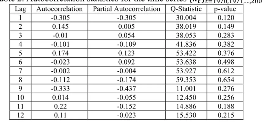
Table 2. Autocorrelation statistics for the time series 𝑘∗
, ,…, .
Lag Autocorrelation Partial Autocorrelation Q-Statistic p-value
1 -0.305 -0.305 30.004 0.120 2 0.145 0.005 38.019 0.149 3 -0.01 0.054 38.053 0.283 4 -0.101 -0.109 41.836 0.382 5 0.174 0.123 53.422 0.376 6 -0.023 0.092 53.638 0.498 7 -0.002 -0.004 53.927 0.612 8 -0.112 -0.174 59.353 0.654 9 -0.333 -0.437 11.001 0.276 10 0.014 -0.055 12.450 0.256 11 0.22 -0.152 14.886 0.188 12 0.11 -0.023 15.530 0.215 ‐6,25 ‐4,25 ‐2,25 ‐0,25 1,75 3,75 5,75 1970 1975 1980 1985 1990 1995 2000
In Table 2, Ljung and Box Q-statistic suggests that a pure random walk for the first difference is accepta-ble. So, we model 𝒌𝒕 as 𝒌𝒕∗ 0. 375 𝒕∗, where
the estimate for the standard deviation of 𝒕∗ is 0.68.
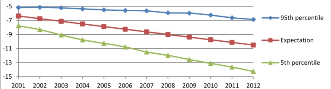
Figure 2 represents the evolution that we predict for 𝒌𝒕 for years 2001-2012 which has been elaborated by
using the bootstrapping procedure for ARIMA time series described in [29].
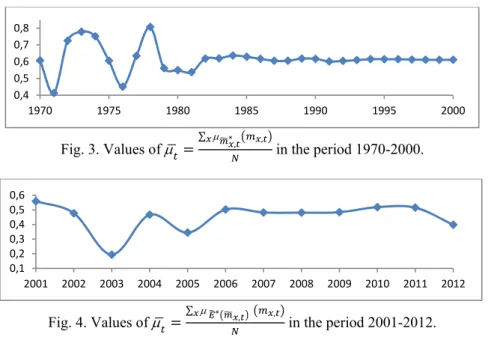
We now check the capability of our extension of the LC model to fit the central rate of mortality, 𝑚 , , into
the sample used to adjust the coefficients, 𝑡 1970,1971, … ,2000 but also its performance in out-of-sample predictions at t= 2001,2002,…,2012. We measure this capability with the membership level that the actual central mortality rate 𝑚 , has in its fuzzy
estimate 𝑚∗, , ∗, 𝑚 , . Figure 3 shows the
aver-age of grades of membership, for all aver-age groups, for the period 1970-2000, i.e., ∑ ∗, , , with 𝑁 the number of age groups that have been considered (𝑁 24 ). Likewise, Figure 4 represents, for 𝑡 2001, … ,2012 , the values of ∑ ∗ , , , where the central rate of mortality has been forecasted by using 𝐸∗ 𝒌
𝒕 , and so, with (12a)-(12b).
Figure 3 shows that the mean grade of membership until the middle of the 80s oscillates, depending on the year, between 0.4 and 0.8. Subsequently, remains always around 0.6. In Figure 4, where we also predict central mortality rates with (12a)-(12b), we can check that with the exception of 2003 and 2005, the average
grade of membership of the real observed central rates of mortality in 𝐸∗ 𝑚
, is at least 0.4. Therefore, it
can be said that the capability of the model to fit the central mortality rates in the sample as well as to ex-trapolate them for a period of more than 10 years is reasonably good.
Table 3 shows the TFN predictions for the central mortality rates of year 2010 that come from 𝐸∗ 𝒌
𝒕
and from the bounds of 𝑘∗, % 𝑘∗, %, 𝑘∗, %, i.e.
we forecast the mathematical expectation and the 10% fuzzy-probabilistic confidence interval of 𝑚 , . For
example, if we consider the age group 30,34 : 𝐸∗ 𝑚
, , 0.00176, 0.00053, 0.00087
which means that the forecasted mean of the cen-tral rate of mortality in the year 2010 is approxi-mately 0.00176, although it can vary between 0.00123 and 0.00263. Likewise, 𝑚∗, %, , has as lower and upper bounds, 𝑚∗, %, , and 𝑚∗, %, , , the TFNs (0.00168, 0.00051, 0.00075) and (0.00184, 0.00055, 0.00100), respectively, i.e. the real central mortality rate in the year 2010 is contained, with a probability of 90%, between approximately 0.00168, in the most optimistic scenario, and approxi-mately 0.00184, in the most pessimistic scenario. If we were using the basic LC model, which only takes into account the uncertainty related to the index 𝒌𝒕, the
re-sults would not be FNs but the real numbers: 0.00176 for the mathematical expectation and [0.00168, 0.00184], for its 90% confidence interval.
Fig. 2. Estimation of the evolution of 𝒌𝒕 for Spanish male population in the period 2001-2012.
‐15 ‐13 ‐11 ‐9 ‐7 ‐5 2001 2002 2003 2004 2005 2006 2007 2008 2009 2010 2011 2012 95th percentile Expectation 5th percentile
Fig. 3. Values of ∑ ∗, , in the period 1970-2000.
Fig. 4. Values of ∑ ∗ , ,
in the period 2001-2012.
Table 3. TFN approximations of the estimates of 𝐸∗ 𝑚
, and the bounds of 𝑚∗, %, (𝑚∗, %, and 𝑚∗, %, ) for
year 2010.
𝐸∗ 𝑚
, 𝑚∗, %, 𝑚∗, %,
Age Centre Left spread Right spread Centre Left spread Right spread Centre Left spread Right spread [0, 1) 0.00206 0.00063 0.00052 0.00115 0.00035 0.00029 0.00379 0.00116 0.00096 [1, 5) 0.00016 0.00003 0.00003 0.00011 0.00002 0.00002 0.00025 0.00005 0.00005 [5,10) 0.00010 0.00002 0.00002 0.00007 0.00001 0.00002 0.00015 0.00003 0.00003 [10,15) 0.00013 0.00004 0.00002 0.00010 0.00003 0.00001 0.00018 0.00004 0.00002 [15,19) 0.00052 0.00018 0.00011 0.00046 0.00019 0.00010 0.00060 0.00016 0.00013 [20,24) 0.00090 0.00029 0.00030 0.00083 0.00033 0.00028 0.00098 0.00025 0.00033 [25,29) 0.00129 0.00037 0.00055 0.00128 0.00038 0.00055 0.00129 0.00037 0.00056 [30,34) 0.00176 0.00053 0.00087 0.00168 0.00051 0.00075 0.00184 0.00055 0.00100 [35,39) 0.00186 0.00032 0.00047 0.00184 0.00032 0.00049 0.00189 0.00032 0.00045 [40,44) 0.00216 0.00016 0.00015 0.00199 0.00015 0.00016 0.00235 0.00018 0.00015 [45,49) 0.00315 0.00036 0.00008 0.00284 0.00037 0.00007 0.00351 0.00033 0.00009 [50,54) 0.00460 0.00024 0.00024 0.00403 0.00021 0.00021 0.00526 0.00027 0.00027 [55,59) 0.00701 0.00051 0.00037 0.00610 0.00046 0.00032 0.00810 0.00056 0.00042 [60,64) 0.01070 0.00086 0.00058 0.00922 0.00074 0.00050 0.01251 0.00101 0.00068 [65,69) 0.01651 0.00201 0.00077 0.01409 0.00197 0.00066 0.01949 0.00202 0.00091 [70,74) 0.02602 0.00205 0.00144 0.02194 0.00173 0.00124 0.03107 0.00245 0.00169 [75,79) 0.04410 0.00422 0.00352 0.03766 0.00360 0.00327 0.05196 0.00497 0.00377 [80,84) 0.07445 0.00592 0.00556 0.06450 0.00513 0.00526 0.08642 0.00687 0.00584 [85,89) 0.12816 0.00877 0.01264 0.11452 0.00784 0.01353 0.14409 0.00986 0.01129 [90,94) 0.21414 0.01404 0.01994 0.19846 0.01321 0.02159 0.23176 0.01497 0.01781 [95,99) 0.32848 0.03803 0.03485 0.31297 0.04353 0.04175 0.34543 0.03162 0.02684 [100,104) 0.46845 0.05871 0.04225 0.45663 0.06889 0.05097 0.48107 0.04750 0.03266 [105,109) 0.61439 0.05071 0.03279 0.60868 0.05592 0.03249 0.62038 0.04519 0.03311 [110,) 0.72704 0.03900 0.04508 0.72661 0.03941 0.04506 0.72748 0.03858 0.04511 0,4 0,5 0,6 0,7 0,8 1970 1975 1980 1985 1990 1995 2000 0,1 0,2 0,3 0,4 0,5 0,6 2001 2002 2003 2004 2005 2006 2007 2008 2009 2010 2011 2012
Note: (a) stands for ∗
, , 𝑚 , and (b) stands for ∗,, ,% 𝑚, .
Fig. 5. Membership levels ∗ , , 𝑚 , and , ,
∗, % 𝑚 , in 2001-2012.
Figure 5 depicts the membership level of true ob-served values of 𝑚 , , for the period 2001-2012 in
the TFNs 𝐸∗ 𝑚
, , and 𝑚∗, %, , . Such important
age group is not well predicted when the mathematical expectation of the parameter 𝒌𝒕 is used because from
the year 2002 on the forecasted rates never contain the real values, i.e. their grade of membership is always 0. Nevertheless, it does not happen when considering the upper bound of the fuzzy-probabilistic 90% confi-dence interval of 𝑚∗, , %. In this case, membership
levels are never lower than 0.4. We statistically test the capability of 𝐸∗ 𝑚
, to predict actual central
mortality rates for each year t = 2001, 2002,…,2012.
Table 4 shows the results. Following [4], it is desirable that the observed rates 𝑚 , attain membership levels
of at least 0.5, in the fuzzy prediction 𝐸∗ 𝑚 , i.e,
∗ , 𝑚 , 0.5. So, for each year t = 2001,
2002,…,2012 we implement a Wilcoxon rank test for the null hypothesis that the median value of ∗ , 𝑚 , is 0.5. It can be seen in Table 4 that
only in years 2003 and 2012 the median of ∗ , 𝑚 , is under 0.5 and the null hypothesis
is rejected at standard significant levels.
Table 4. Assessment of the capability prediction of 𝐸∗ 𝑚
, with a Wilcoxon rank test in 2001-2012.
Year 𝑊 Median Mean Year 𝑊 Median Mean 2001 92* 0.602 0.656 2007 93 0.414 0.381 2002 141 0.488 0.643 2008 141 0.438 0.256 2003 77** 0.181 0.439 2009 59** 0.534 0.246 2004 140 0.454 0.431 2010 122 0.462 0.233 2005 117 0.165 0.337 2011 67*** 0.521 0.255 2006 61*** 0.528 0.320 2012 62*** 0.202 0.182
Notes: (1) 𝑊 stands for the value of Wilcoxon rank test statistic. (2) “*”, “**” and “***” stand for the rejection of the null hypothesis that the median value of ∗
, 𝑚, is 0.5 with a significance level of 10%, 5% and 1% respectively.
5. Forecasting life expectancy with the fuzzy-random Lee-Carter model
5.1. Calculating life expectancy from fuzzy estimates
of central mortality rates
We now compute probabilities of death or survival and life expectancies after calculating estimates of central mortality rates. Let us denote the width of the age group as 𝑛 years.
To obtain the probability that a person in the age group 𝑥, at calendar year 𝑡, does not reach the follow-ing age group, 𝑞 ,,we have to take into account that
it is a function of 𝑚 , .
𝑞 , ,
, , (15)
where , ∈ 0,1 is the average fraction of the 𝑛 -year period lived by those who died in that period and we will suppose that this coefficient is fixed before-hand. Given that:
𝜕 𝑞, 𝜕𝑚, 𝑛 1 𝑛 1 , 𝑚 , 0 0 0,2 0,4 0,6 0,8 1 2001 2002 2003 2004 2005 2006 2007 2008 2009 2010 2011 2012 (a) (b)
by considering (15) and bearing in mind that 𝑞∗,
is a prediction of a probability, i.e. 𝑞∗, ⊆ 0,1 , we
can obtain the 𝛼-cuts of 𝑞∗, , 𝑞∗, :
𝑞∗, 𝑞∗, 𝛼 , 𝑞∗, 𝛼 max 0, 𝑛 𝑚, ∗ 𝑙 , ∗ 1 𝛼 1 𝑛 1 , 𝑚∗, 𝑙 ∗, 1 𝛼 , min 1, 𝑛 𝑚, ∗ 𝑟 , ∗ 1 𝛼 1 𝑛 1 , 𝑚∗, 𝑟 ∗, 1 𝛼
It may be useful to obtain a triangular approxima-tion for 𝑞∗, , 𝑞∗, 𝑞∗,, 𝑙 ∗,, 𝑟 , ∗ , with: 𝑞∗, , ∗ , ∗, (16a)
In order to obtain the support of 𝑞∗, , we have to
take into account that it is a probability and so, its sup-port must be within the interval [0, 1]. Then:
𝑙 ∗, min 𝑞∗,, , ∗ , , (16b) and: 𝑟 , ∗ min 1 𝑞∗,, , ∗ , , (16c) To determine the probability that a person in the age group 𝑥, at calendar year 𝑡, reaches the following age group, 𝑝 , , from the crisp relationship
𝑝 , 1 𝑞 , , under fuzziness we state
𝑝 , 1 𝑞 , where: 𝑝∗, 𝑝∗, 𝛼 , 𝑝∗, 𝛼 1 𝑞∗, 𝛼 , 1 𝑞∗, 𝛼 From (15a)-(15c), 𝑝∗, 𝑝∗,, 𝑙 ∗,, 𝑟 , ∗ : 𝑝∗, 1 𝑞∗,; 𝑙 ∗, 𝑙 , ∗ ; 𝑟 , ∗ 𝑟 , ∗
The life expectancy of a person in the age group 𝑥, at calendar year 𝑡, 𝑒 , can be calculated with the
expres-sion: 𝑒, ∑ ∏ 1 𝑞, 𝑛 𝑛 , 𝑞, (17) As: 𝜕𝑒, 𝜕 𝑞, 1 𝑞, 𝑛 𝑛 , 1 𝑞, 𝑛 𝑛 , 𝑞,
it turns out that 𝑒 , is a decreasing function of 𝑞,
(and so, of its linked central mortality rate).
By evaluating (17) with 𝑞∗, , we will obtain a
fuzzy estimate for 𝑒 , , 𝑒̃∗, . Moreover, it is
straight-forward to see that its 𝛼 –cuts, 𝑒∗, , are:
𝑒∗, 𝑒∗, 𝛼 , 𝑒∗, 𝛼
1 𝑞, 𝛼 𝑛 𝑛 , 𝑞, 𝛼 , 1 𝑞, 𝛼 𝑛 𝑛 , 𝑞, 𝛼
A TFN approximation of 𝑒̃∗, , 𝑒̃∗,
𝑒∗,, 𝑙∗,, 𝑟∗, , can be obtained by using (6):
𝑒∗, ∑ ∏ 1 𝑞∗, 𝑛 𝑛 , 𝑞∗, (18a) 𝑙∗, 1 𝑞∗, 𝑛 , 1 𝑞∗, 𝑛 𝑛 , 𝑞∗, 𝑟 ∗, (18b) 𝑟∗, 1 𝑞∗, 𝑛 , ∑ ∏ 1 𝑞∗, 𝑛 𝑛 , 𝑞∗, 𝑙 ∗, (18c) Of course, if in (18a)-(18c) we take as a prediction of the index 𝒌𝒕 its mathematical expectation, 𝑘∗
𝐸∗ 𝒌
𝒕 , we will obtain a fuzzy estimate of life
expec-tation that we symbolize as 𝐸∗ 𝑒̃ , ∗ .
If the prediction of the mortality trend comes from its probabilistic confidence interval, 𝑘∗,
𝑘∗, , 𝑘∗, , we can built up a fuzzy-probabilistic confidence interval of the life expectancy 𝑒∗,,
𝑒∗,, , 𝑒∗,, . In the common case where the sensitivity of the central rate of mortality respect to changes in the index 𝒌𝒕 is strictly positive, i.e. 𝑏∗>0 (𝑏∗ 𝑙 ∗0),
𝑘∗, will determinate 𝑒∗,, , whereas 𝑘∗, will de-fine the lower life expectancy 𝑒∗,, .
5.2. Predicting life expectancies of Spanish male
pop-ulation in 2001-2012
Tables 5 and 6 show the estimates for the mean value and the 90% confidence fuzzy-probabilistic in-terval of the life expectancy for the age groups 0, 1 and 65, 69 during the period 2001-2012. These ages are significantly important because they are con-sidered in order to quantify life expectancy at birth and at retirement, respectively. If only the centres of the fuzzy life expectancies are considered, predictions that come from the basic LC method are found. So, for ex-ample, the point estimate for 𝑒 , , is 78.19 years
and the 90% confidence probabilistic interval is [76.56, 79.75] years. The fuzzy-random extension of the LC
model allows introducing the fuzziness into the coef-ficients 𝑎 and 𝑏 and, as a consequence, point pre-dictions and probabilistic interval prepre-dictions, as well, are fuzzified. So, the projection of 𝑒 , , is the
TFN (78.19, 1.25, 1.30) years, whereas the lower and upper bounds of the 90% confidence fuzzy probabilis-tic interval are, respectively (76.56, 1.19, 1.28) and (79.75, 1.34, 1.33).
Table 5. TFN approximation of the estimates of 𝐸∗ 𝑒̃ , , ∗ and 𝑒̃
, ,
∗, %, with lower and upper bounds 𝑒̃ , , ∗, % and 𝑒̃∗, %, ,, in 2001-2012. 𝐸∗ 𝑒̃ , , ∗ 𝑒̃ , , ∗ % 𝑒̃∗, , %
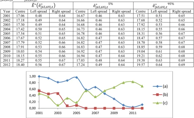
Year Centre Left spread Right spread Centre Left spread Right spread Centre Left spread Right spread 2001 76.31 1.18 1.28 75.73 1.17 1.28 76.96 1.20 1.28 2002 76.49 1.19 1.28 75.72 1.17 1.28 77.20 1.21 1.29 2003 76.66 1.19 1.28 75.75 1.17 1.28 77.54 1.22 1.29 2004 76.84 1.20 1.28 75.82 1.18 1.28 77.85 1.23 1.30 2005 77.01 1.20 1.29 75.89 1.18 1.28 78.07 1.24 1.30 2006 77.18 1.21 1.29 75.94 1.18 1.28 78.29 1.25 1.30 2007 77.35 1.21 1.29 75.94 1.18 1.28 78.60 1.27 1.31 2008 77.52 1.22 1.29 75.97 1.18 1.28 78.80 1.28 1.31 2009 77.69 1.23 1.29 76.10 1.18 1.28 79.05 1.29 1.32 2010 77.85 1.23 1.30 76.13 1.18 1.28 79.28 1.31 1.32 2011 78.02 1.24 1.30 76.26 1.18 1.28 79.50 1.32 1.33 2012 78.19 1.25 1.30 76.56 1.19 1.28 79.75 1.34 1.33 Table 6. TFN approximation of the estimates of 𝐸∗ 𝑒̃
, , ∗ and 𝑒̃
, ,
∗, % , with lower and upper bounds
𝑒̃∗, %, , and 𝑒̃∗, %, ,, in 2001-2012. 𝐸∗ 𝑒̃ , , ∗ 𝑒̃ , , ∗ % 𝑒̃ , , ∗ %
Year Centre Left spread Right spread Centre Left spread Right spread Centre Left spread Right spread 2001 17.06 0.48 0.64 16.67 0.46 0.63 17.51 0.51 0.65 2002 17.18 0.49 0.64 16.66 0.46 0.63 17.68 0.52 0.65 2003 17.30 0.49 0.64 16.68 0.46 0.63 17.92 0.53 0.66 2004 17.42 0.50 0.65 16.73 0.46 0.63 18.15 0.55 0.66 2005 17.54 0.51 0.65 16.78 0.46 0.63 18.31 0.56 0.67 2006 17.67 0.52 0.65 16.82 0.47 0.63 18.47 0.57 0.67 2007 17.79 0.52 0.66 16.82 0.47 0.63 18.70 0.58 0.67 2008 17.91 0.53 0.66 16.83 0.47 0.63 18.85 0.59 0.68 2009 18.03 0.54 0.66 16.92 0.47 0.63 19.04 0.61 0.68 2010 18.15 0.55 0.66 16.94 0.47 0.64 19.21 0.62 0.68 2011 18.27 0.55 0.67 17.03 0.48 0.64 19.38 0.63 0.69 2012 18.40 0.56 0.67 17.24 0.49 0.64 19.57 0.64 0.69
Note: (a) stands for ∗ ̃ , ,
∗ 𝑒 , , , (b) stands for 𝜇̃∗, %, , 𝑒 , , and (c) stands for 𝜇̃∗,, ,% 𝑒 , , .
Fig. 6. Membership levels ∗ ̃ , , ∗ 𝑒 , , , 𝜇̃∗, %, , 𝑒 , , and 𝜇 ̃∗,, ,% 𝑒 , , in 2001-2012. 0,00 0,20 0,40 0,60 0,80 1,00 2001 2003 2005 2007 2009 2011 (a) (b) (c)
Note: (a) stands for ∗ ̃ , ,
∗ 𝑒 , , , (b) stands for 𝜇̃ , ,
∗, % 𝑒 , , and (c) stands for 𝜇̃ , ,
∗, % 𝑒 , , .
Fig. 7. Membership levels ∗ ̃ , ,
∗ 𝑒 , , , 𝜇̃∗, %, , 𝑒 , , and 𝜇̃∗, ,%, 𝑒 , , in 2001-2012.
Table 7. Assessment of the capability prediction of 𝐸∗ 𝑒̃ ,
∗ with a Wilcoxon rank test for the period
2001-2012. Capability prediction of 𝐸∗ 𝑒̃
,
∗ per years
Year 𝑊 Median Mean Year 𝑊 Median Mean 2001 92* 0.602 0.718 2007 93 0.414 0.589 2002 141 0.488 0.656 2008 141 0.438 0.586 2003 77** 0.181 0.338 2009 59*** 0.534 0.555 2004 140 0.454 0.653 2010 122 0.462 0.445 2005 117 0.165 0.440 2011 67*** 0.521 0.443 2006 61*** 0.528 0.699 2012 62*** 0.202 0.409 Capability prediction of 𝐸∗ 𝑒̃ , , ∗ and 𝐸∗ 𝑒̃ , , ∗ on life expectancy
at birth and retirement
Median Mean 𝑊 𝐸∗ 𝑒̃ , , ∗ 0.628 0.567 37 𝐸∗ 𝑒̃ , , ∗ 0.655 0.609 19
Notes: (1) Each year has 24 predictions on life expectations, one per age group. (2) Each age group has 12 predictions available, one for each assessed year. (3) 𝑊 stands for the value of Wilcoxon rank test statistic. (4) “*”, “**” and “***” stand for the rejection of the null hypothesis that median value of ∗ ̃
,
∗ 𝑒, is 0.5 with a significance level of 10%, 5% and 1% respectively.
Figures 6 and 7 represent the membership level of true observed values for life expectancies, 𝑒 , , into
their estimates 𝐸∗ 𝑒̃ , ∗ , 𝑒̃ , ∗, % and 𝑒̃ , ∗, %. Concretely,
we take the estimates calculated in Tables 5 and 6. We can check that 𝑒 , , is fitted quite accurately by
𝐸∗ 𝑒̃ , ,
∗ from 2001 to 2005. On the other hand,
from 2006 to 2012, 𝜇 ∗ ̃ , ,
∗ 𝑒 , , decreases to
values near 0. However, we can also remark that in those years the membership level of 𝑒 , , into the
TFN 𝑒̃∗, %, , stands clearly up to 0.5. Likewise, for 65, 69 , Figure 7 shows that 𝐸∗ 𝑒̃
, , ∗ fits 𝑒
, ,,
from 2006 to 2012, with clearly satisfactory member-ship levels that are usually up 0.8. It is true that 𝜇 ∗ ̃
, ,
∗ 𝑒 , , has low values in the years
2003 and 2005 but they are compensated by the greater membership levels of 𝜇 ̃
, ,
∗, % 𝑒 , , . In a
similar way as in subsection 4.3., we statistically test
the capability of fuzzy mean life expectancies to pre-dict actual life expectations at t = 2001,2002,…, 2012. Again, for each year t =2001,2002,…,2012 we imple-ment a Wilcoxon rank test with the null hypothesis that the median value of ∗ ̃∗, 𝑚 , 0.5. Table
7 shows that, except for the year 2003, in the years where the median of ∗ , 𝑚 , is under 0.5, we
cannot reject the null hypothesis. On the other hand, in the years 2001, 2007, 2010 and 2011, there are statis-tical evidences that the median is above 0.5.
Due to the interest in actuarial analyses in life ex-pectancy both at birth and at retirement, we test the quality of the prediction by 𝐸∗ 𝑒̃
,
∗ in years [0,1) an
[65,69). The results are also collected in Table 7. We can check that the median and mean membership lev-els of observed life expectancies in the period 2001-2012 are consistently above 0.5. However, the Wil-coxon rank test does not reject in both age groups that 𝜇 ∗ ̃ , ∗ 𝑒 , 0.5. 0,00 0,20 0,40 0,60 0,80 1,00 2001 2003 2005 2007 2009 2011 (a) (b) (c)
6. Empirical assessment of the Fuzzy Random Lee-Carter model in eight Western European
countries1
6.1. Methodological considerations
In this section we make a comparative assessment on the prediction capability of our proposed fuzzy-ran-dom extension of the LC model (FRLC) with both the basic LC (BLC) in [26] and the pure fuzzy LC version in [22] (FKSLC). Let us remark that BLC only con-siders random uncertainty ofcoefficients 𝑘 . On the other hand, FKSLC introduces fuzzy uncertainty in all the coefficients of the LC model by means of symmet-rical TFNs. Likewise, FKSLC handles uncertainty with the weakest t-norm instead of the commonly used minimum operator.
To carry out the analysis, we use central mortality rates collected separately for men and women in eight Western Europe countries (i.e. we use 16 databases) from [38] (http://www.mortality.org). As we made in sections 4 and 5 for the case of Spanish male popula-tion, we fit the model parameters by using central mor-tality rates in the period 1970-2000 and we test models out-of-sample performance during 2001-2012. Ages are again grouped in 5 year intervals, except for ages lower than 1 year, for ages from 1 to 5 years and for ages greater or equal to 110 years.
We assess two aspects regarding the fitting quality of the models:
Item 1. We measure and compare models’ perfor-mance to make point predictions on central mortality rates and life expectancies. This is made by using the conventional error measures: Root Mean Squared Er-ror (RMSE), Normalised Mean Squared ErEr-ror (NMSE) and Mean Absolut Error (MAE). We con-sider these point predictions: the expectation for BLC, the core of the fuzzy expectation for FRLC and, finally, the core of the fuzzy prediction for FKSLC. Notice that point predictions by BLC and FRLC are the same by definition. So, in fact, we are making a comparison of a couple of predictive methods: BLC/FRLC versus FKSLC. Following [32], this pairwise comparison be-tween techniques is made with both a sign test (Wins/Losses) and a Wilcoxon rank test.
Item 2. We evaluate the capability of BLC, FRLC and FKSLC to predict future values of 𝑚 ,, and 𝑒 ,
by means of confidence intervals. In this second item, we measure the accuracy of a method as the rate of
1 This section is especially benefited by the helpful
sugges-tions of one anonymous referee.
right predictions on 𝑚 , or 𝑒 , through confidence
intervals estimates provided by the methods. In this regard, let us make the following remarks: - BLC only considers random uncertainty of 𝑘 . So, after establishing a significance level 𝜀, that in our nu-merical assessment will be 10%, BLC predicts life variables as a 1 𝜀 confidence interval like in (14).
- FRLC estimates the lower and upper bounds of the 1 𝜀 confidence interval by means of two TFNs. To obtain standard confidence interval predictions, we transform these estimates into a conventional confi-dence interval that comes from the convex hull, 𝐶 , of the expected intervals (4b) corresponding to and 1 percentiles of fuzzy predictions (5% and 95% in our numerical application). So, for 𝑚 , , the 1 𝜀
confidence interval prediction is 𝐶 𝑒 𝑚∗,, ∪ 𝑒 𝑚∗,,
. Analogously, the 1 𝜀 confidence in-terval prediction of 𝑒 , is 𝐶 𝑒 𝑒̃ ,
∗,
∪ 𝑒 𝑒̃∗,, . For example, the life expectancy at birth of a Spanish man born in 2004 for 𝜀 10% is built up from
𝑒̃∗, , % 75.82, 1.18,1.28 and
𝑒̃∗, , % 77.85,1.23,1.30 (see Table 5). We
easily find that 𝑒 𝑒̃∗, , % 75.23, 76.46 and
𝑒 𝑒̃∗, , % 77.23, 78,50 . Then, the 90%
confidence interval prediction for 𝑒 , , is (in
years):
𝐶 75.23, 76.46 ∪ 77.23, 78,50 75.23, 78.50
- FKSLC directly predicts mortality variables as FNs. The expected interval of the FN obtained from this method is taken as its confidence interval.
The analysis of both questions is developed in two levels:
a) In each population, we independently assess the predictive capability of each method. For a given pop-ulation we must predict 24 variables for each of the 12 years that testing period 2001-2012 comprises. In each year we find the mean value of the accuracy measures and so, for each population, we have 12 available mean values of accuracy (one per year). The results that we find in this case are exclusive to the population studied.
b) We will use the mean results of the accuracy pre-dictions within the whole period 2001-20012 of all populations to make an inter-population assessment. It may lead to extract more general conclusions about the method performance. In this case, we will work with a sample of 16 different goodness of fit measures and we will extract more general conclusions.
Following [17] and [18], an adequate non-paramet-rical test to carry out this kind of analysis is the Fried-man rank test (FriedFried-man 2 and Iman-Davenport F
statistics) that may be completed by the pairwise com-parisons that allow using Friedman ranks (Z-score). Likewise, given that FRLC and FKSLC are extensions of BLC, we will implement the multiple sign test de-scribed in [17] where the control technique is BLC.
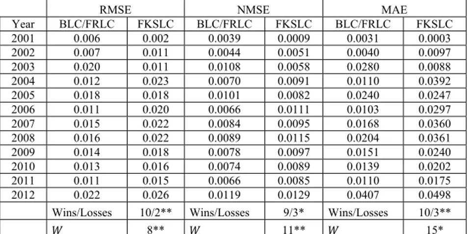
Table 8a. Mean RMSE, NMSE and MAE (per years) of central mortality rates point predictions for Spanish men by the evaluated methods (Item 1).
RMSE NMSE MAE
Year BLC/FRLC FKSLC BLC/FRLC FKSLC BLC/FRLC FKSLC 2001 0.006 0.002 0.0039 0.0009 0.0031 0.0003 2002 0.007 0.011 0.0044 0.0051 0.0040 0.0097 2003 0.020 0.011 0.0108 0.0058 0.0280 0.0088 2004 0.012 0.023 0.0070 0.0091 0.0110 0.0392 2005 0.018 0.018 0.0101 0.0082 0.0240 0.0247 2006 0.011 0.020 0.0066 0.0111 0.0103 0.0297 2007 0.015 0.022 0.0084 0.0095 0.0168 0.0360 2008 0.016 0.022 0.0089 0.0115 0.0204 0.0361 2009 0.014 0.018 0.0078 0.0097 0.0151 0.0240 2010 0.013 0.016 0.0074 0.0089 0.0139 0.0202 2011 0.011 0.015 0.0066 0.0085 0.0110 0.0175 2012 0.022 0.026 0.0119 0.0129 0.0407 0.0498 Wins/Losses 10/2** Wins/Losses 9/3* Wins/Losses 10/3**
𝑊 8** 𝑊 11** 𝑊 15*
Notes: (1) “Wins/Losses” stands for the number of cases in which BLC and FRLC point predictions are better/worse than FKSLC. (2) 𝑊 stands for the value of the Wilcoxon rank test statistic. (3) “*”, “**” and “***” stand for the rejection of the null hypothesis with a significance level of 10%, 5% and 1% respectively.
Table 8b. Mean RMSE, NMSE and MAE (per years) of life expectancy point predictions for Spanish men by the evaluated methods (Item 1).
RMSE NMSE MAE
Year BLC/FRLC FKSLC BLC/FRLC FKSLC BLC/FRLC FKSLC 2001 0.152 0.246 1.51E-04 2.45E-04 0.122 0.160 2002 0.194 0.232 1.91E-04 2.30E-04 0.149 0.155 2003 0.327 0.218 3.21E-04 2.16E-04 0.287 0.202 2004 0.190 0.400 1.83E-04 3.90E-04 0.173 0.287 2005 0.270 0.344 2.61E-04 3.35E-04 0.235 0.264 2006 0.348 0.647 3.30E-04 6.19E-04 0.235 0.484 2007 0.306 0.571 2.89E-04 5.44E-04 0.251 0.404 2008 0.443 0.754 4.14E-04 7.38E-04 0.308 0.561 2009 0.560 0.889 5.18E-04 8.30E-04 0.008 0.010 2010 0.712 1.060 6.51E-04 9.79E-04 0.007 0.009 2011 0.769 1.127 6.98E-04 1.03E-03 0.007 0.008 2012 0.703 1.056 6.36E-04 9.75E-04 0.012 0.013
Wins/Losses 11/1* Wins/Losses 11/1** Wins/Losses 11/1**
𝑊 9** 𝑊 9** 𝑊 5**
Notes: (1) “Wins/Losses” stands for the number of cases in which BLC and FRLC point predictions are better/worse than FKSLC (2) 𝑊 stands for the value of the Wilcoxon rank test statistic. (3) “*”, “**” and “***” stand for the rejection of the null hypothesis with a significance level of 10%, 5% and 1% respectively.
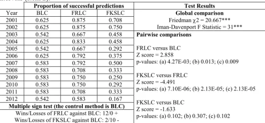
Table 8c. Mean proportion of successful predictions on central mortality rates of BLC, FRLC and FKSLC with confidence intervals (Item 2).
Proportion of successful predictions Test Results
Year BLC FRLC FKSLC Global comparison
Friedman 2 = 20.667*** Iman-Davenport F Statistic = 31*** 2001 0.625 0.875 0.708 2002 0.625 0.875 0.750 2003 0.542 0.667 0.458 Pairwise comparisons FRLC versus BLC Z score = 2.858
p-values: (a) 4.27E-03; (b) 0.013; (c) 0.009 FKSLC versus FRLC
Z score = -4.491
p-values: (a) 7.10E-06; (b) 2.13E-05; (c) 2.13E-05 FKSLC versus BLC Z score = -1.633 p-values: (a) 0.102; (b) 0.307; (c) 0.102 2004 0.625 0.833 0.458 2005 0.542 0.667 0.292 2006 0.625 0.792 0.375 2007 0.583 0.792 0.500 2008 0.583 0.708 0.333 2009 0.583 0.750 0.250 2010 0.583 0.750 0.292 2011 0.583 0.708 0.333 2012 0.542 0.583 0.167
Multiple sign test (the control method is BLC)
Wins/Losses of FRLC against BLC: 12/0 + Wins/Losses of FKSLC against BLC: 2/10 -
Notes: (1) Friedman 2 follows a Squared-Chi with 2 grades of freedom and Iman-Davenport F follows a Snedecor F with 2(24) grades of freedom. (2) “*”, “**” and “***” stand for the rejection of the null hypothesis with a significance level of 10%, 5% and 1% respectively. (3) (a) indicates standard p-value, and (b) and (c) Nemenyi and Holm p-value corrections for multiple pairwise comparisons. (4) “+” indicates that the evaluated method outperforms the control method with at least at 10% significance level whereas “-“ indicates that the evaluated method under-performs the control method with at least at 10% significance level.
Table 8d. Mean proportion of successful predictions on life expectancies of BLC, FRLC and FKSLC with confi-dence intervals (Item 2).
Proportion of successful predictions Test Results
Year BLC FRLC FKSLC Global comparison
Friedman 2 = 8.0417*** Iman-Davenport F Statistic = 5.5431** 2001 0.792 0.958 0.958 2002 0.833 0.958 0.958 2003 0.667 0.792 0.667 Pairwise comparisons FRLC versus BLC Z score = 2.756 p-values: (a) 0.006; (b) 0.018; (c) 0.012 FKSLC versus FRLC Z score = -3.878
p-values: (a) 6.88E-05; (b) 2.06E-04; (c) 1.38E-04 FKSLC versus BLC Z score = -1.123 p-values: (a) 0.262; (b) 0.785; (c) 0.262 2004 0.833 0.958 0.625 2005 0.750 0.833 0.458 2006 0.875 0.958 0.375 2007 0.833 0.917 0.583 2008 0.833 0.875 0.292 2009 0.875 0.917 0.292 2010 0.875 0.958 0.250 2011 0.833 0.958 0.250 2012 0.833 0.875 0.167
Multiple sign test (the control method is BLC)
Wins/losses of FRLC against BLC: 12/0 + Wins/losses of FKSLC against BLC: 3/9
Notes: (1) Friedman 2 follows a Squared-Chi with 2 grades of freedom and Iman-Davenport F follows a Snedecor F with 2(24) grades of freedom (2) “*”, “**” and “***” stand for the rejection of the null hypothesis with a significance level of 10%, 5% and 1% respectively. (3) (a) indicates standard p-value, and (b) and (c) Nemenyi and Holm p-value corrections for multiple pairwise comparisons. (4) “+” indicates that the evaluated method outperforms the control method with at least at 10% significance level whereas “-“ indicates that the evaluated method under-performs the control method with at least at 10% significance level.
6.2. Comparison of BLC, FRLC and FKSLC for
each population
We now show the adequacy of the three LC meth-ods evaluated in 16 populations. We present in a more detailed way the results corresponding to Spanish male population (Table 8a-8d) and a summary table for all the analysed countries (Tables (9a-9e)).
Regarding item 1, we can check in Tables 8a and 8b that for Spanish male population, BLC/FRLC point
predictions of 𝑚 , , and 𝑒 , are, generally, more
accu-rate than those by FKSLC and this best adjustment has a consistent statistical significance. Furthermore, Ta-ble 9a shows that in the studied populations, as in the case of Spanish men, point predictions of 𝑚 , from
BLC/FRLC are normally better than those from FKSLC and this fact has also statistical significance. We can appreciate three exceptions: Belgian male population, where FKSLC beats BLC/FRLC with a consistent statistical level and UK and Netherlands
fe-male populations where we do not appreciate any sig-nificant better method. Table 9c shows that in the pre-diction of 𝑒 ,, it is less clear that BLC/FRLC
predic-tions are better than those by FKSLC. BLC/FRLC beats FKSLC with a clear statistical significance in eight populations but in five populations FKSLC works clearly better. Likewise, in three populations the possible superior performance of a given method has no statistical significance.
In regards to item 2, in Spanish male population, we can check in Tables 8c and 8d that Friedman rank test rejects the homogeneity in the accuracy of the predic-tions over analysed life variables by the three assessed methods. Pairwise comparisons lead us to conclude that FRLC makes better interval predictions than BLC and FKSLC. However, despite the fact that we can de-tect that BLC beats FKSLC, this superior performance has no statistical significance. In this sense, multiple sign test shows that our method clearly beats the con-trol method and, on the other hand, the concon-trol method seems to be superior to FKSLC but without statistical significance. Tables 9c-9d show that those facts are common to all studied populations. So, Friedman 2 and Iman-Davenport statistics always reject the homo-geneity of the prediction capability by the three meth-ods. This fact applies for 𝑚 , , and for 𝑒 , . Pairwise
Friedman ranks tests show that the prediction on cen-tral mortality rates by FRLC beats significantly those obtained by BLC and FKSLC. Likewise, we can also check that BLC usually makes more accurate interval predictions than FKSLC but that better performance, except for the case of French women, has not statisti-cal significance.
In the analysis of life expectancy predictions, pair-wise Friedman ranks tests (see Table 9d) reveal that FRLC predicts confidence intervals consistently better than other methods in most populations. In any case, it is also true that in French and Italy female popula-tions and Portugal male population (Netherlands male population) the greater accuracy of FRLC over BLC (FKSLC over FRLC) is not statistically significant. We can also check that in most cases BLC includes more percentage of observed values of 𝑒 , than
FKSLC but it is only statistically relevant in five pop-ulations. However, in the case of Netherlands male population, FKSLC model predicts life expectancies better than BLC with a clear significance level. Re-sults of multiple sign tests in Table 9e show that our method improves significantly BLC (the control method) whereas this clearly does not follow with FKSLC method.
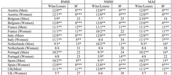
Table 9a. Results of sign and Wilcoxon tests on the difference between the accuracy of point estimates on central mortality rates by BLC/FRLC and FKSLC in the period 2001-2012 (Item 1).
RMSE NMSE MAE
Wins/Losses 𝑊 Wins/Losses 𝑊 Wins/Losses 𝑊
Austria (Men) 12/0** 0*** 12/0** 0*** 12/0** 0*** Austria (Women) 12/1** 0*** 12/0** 0*** 12/0** 0*** Belgium (Men) 3/9* 23 5/7 25 2/10** 18 Belgium (Women) 12/0** 0*** 12/0** 0*** 12/0** 0*** France (Men) 11/1** 12** 11/1** 11** 11/1** 11** France (Women) 11/1** 11** 10/2** 22 11/1** 11** Italy (Men) 12/0** 0*** 12/0** 0*** 12/0** 0*** Italy (Women) 11/1** 8** 8/4 34 11/1** 3*** Netherlands (Men) 9/3* 15* 10/2** 11** 9/3* 16* Netherlands (Women) 8/4 31 8/4 28 8/4 30 Portugal (Men) 10/2** 22 9/3* 24 10/2** 16* Portugal (Women) 4/8 23 3/9* 14** 4/8 22 Spain (Men) 10/2** 8** 9/3* 11** 10/2** 15* Spain (Women) 12/0** 0*** 12/0** 0*** 12/0** 0*** UK(Men) 11/1** 11** 12/0** 0*** 11/1** 12** UK (Women) 5/7 27 6/6 38 5/7 31
Notes: (1) “Wins/Losses” are accounted from the perspective of BLC/FRLC. (2) “*”, “**” and “***” stand for the rejection of the null hypothesis with a significance level of 10%, 5% and 1% respectively.
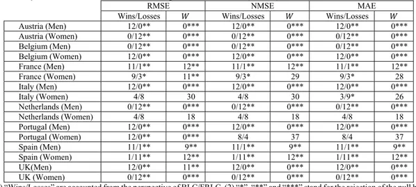
Table 9b. Results of sign and Wilcoxon tests on the difference between the accuracy of point estimates on life expectancies by BLC/FRLC and FKSLC in the period 2001-2012 (Item 1).
RMSE NMSE MAE
Wins/Losses 𝑊 Wins/Losses 𝑊 Wins/Losses 𝑊
Austria (Men) 12/0** 0*** 12/0** 0*** 12/0** 0*** Austria (Women) 0/12** 0*** 0/12** 0*** 0/12** 0*** Belgium (Men) 0/12** 0*** 0/12** 0*** 0/12** 0*** Belgium (Women) 12/0** 0*** 12/0** 0*** 12/0** 0*** France (Men) 11/1** 12** 11/1** 12** 11/1** 12** France (Women) 9/3* 11** 9/3* 29 9/3* 28 Italy (Men) 12/0** 0*** 12/0** 0*** 12/0** 0*** Italy (Women) 4/8 30 4/8 30 3/9* 26 Netherlands (Men) 0/12** 0*** 0/12** 0*** 0/12** 0*** Netherlands (Women) 4/8 18 4/8 18 4/8 18 Portugal (Men) 12/0** 0*** 12/0** 0*** 12/0** 0*** Portugal (Women) 12/0** 0*** 8/4 37 8/4 37 Spain (Men) 11/1** 9** 11/1** 9** 11/1** 9** Spain (Women) 1/11** 12** 1/11** 12** 1/11** 12** UK(Men) 12/0** 11** 12/0** 0*** 12/0** 0*** UK (Women) 0/12** 0*** 0/12** 0*** 0/12** 0***
Notes: (1) “Wins/Losses” are accounted from the perspective of BLC/FRLC. (2) “*”, “**” and “***” stand for the rejection of the null hypothesis with a significance level of 10%, 5% and 1% respectively.
Table 9c. Results of Friedman rank tests and pairwise Friedman rank tests for the accuracy of the confidence interval predictions on central mortality rates by BLC, FRLC and FKSLC in sample populations in the period 2001-2012 (Item 2).
Pairwise Z scores from Friedman ranks Friedman test
FRLC vs BLC FKSLC vs FRLC FKSLC vs BLC Friedman 2 Iman-Davenport F Austria (Men) 3.164*** -3.776*** -0.612 8.542** 6.079*** Austria (Women) 3.062*** -4.082*** -1.021 14.083*** 15.621*** Belgium (Men) 2.654** -4.491*** -1.837 18.375*** 35.933*** Belgium (Women) 2.654** -4.695*** -2.041 22.167*** 133.026*** France (Men) 2.858** -4.491*** -1.633 20.660*** 68.042*** France (Women) 2.449** -4.695*** -2.245* 20.000*** 55.000*** Italy (Men) 2.654** -4.491*** -1.837 16.420*** 23.828*** Italy (Women) 2.654** -4.695*** -2.041 22.167*** 133.026*** Netherlands (Men) 2.858** -4.491*** -1.633 20.667*** 68.208*** Netherlands (Women) 2.654** -4.287*** -1.633 10.830*** 9.046*** Portugal (Men) 2.654** -4.695*** -2.041 22.167*** 133.026*** Portugal (Women) 3.062*** -3.674*** -0.612 15.500*** 20.059*** Spain (Men) 2.858** -4.491*** -1.633 20.667*** 68.208*** Spain (Women) 3.062*** -4.082*** -1.021 14.083*** 15.621*** UK(Males) 2.654** -4.082*** -1.429 5.417* 3.207* UK (Women) 2.654** -4.491*** -1.837 16.417*** 23.815***
Notes: (1) “*”, “**” and “***” stand for the rejection of the null hypothesis with a significance level of 10%, 5% and 1% respectively. (2) Friedman 2 follows a Squared-Chi with 2 grades of freedom and Iman-Davenport F follows a Snedecor F with 2(24) grades of freedom. Table 9d. Results of Friedman rank tests and pairwise Friedman rank tests for the accuracy of the confidence interval predictions on life expectancies by BLC, FRLC and FKSLC in sample populations in the period 2001-2012 (Item 2).
Pairwise Z scores from Friedman ranks Friedman test
FRLC vs BLC FKSLC vs FRLC FKSLC vs BLC Friedman 2 Iman-Davenport F Austria (Men) 3.164*** -4.185*** -1.021 19.042*** 42.247*** Austria (Women) 2.449** -3.266*** -0.816 7.750** 5.246** Belgium (Men) 2.143* -4.287*** -2.143* 18.370*** 35.892*** Belgium (Women) 2.245* -4.491*** -2.245* 20.100*** 56.692*** France (Men) 2.347* -3.470*** -1.123 12.540*** 12.037*** France (Women) 1.123 -3.572*** -2.449** 9.375*** 7.051*** Italy (Men) 2.449** -4.899*** -2.449** 24.000*** *** Italy (Women) 2.041 -2.449** -0.408 6.500** 4.086** Netherlands (Men) 4.695*** -2.041 2.654** 22.167*** 133.026***