Scuola di Dottorato in Ingegneria “Leonardo da Vinci”
Corso di Dottorato di Ricerca in
Ingegneria dell’Informazione: Elettronica, Informatica,
Telecomunicazioni
Tesi di Dottorato di Ricerca
Computational intelligence techniques for
maritime and coastal remote sensing
Autore:
Linda Corucci ___________________
Relatori:
Prof. Beatrice Lazzerini ____________________ Prof. Francesco Marcelloni ____________________ Ing. Andrea Masini ____________________ Ing. Marco Cococcioni ____________________
Anno 2011 SSD ING-INF/05
i
The aim of this thesis is to investigate the potential of computational intelligence techniques for some applications in the analysis of remotely sensed multi-spectral images. In particular, two problems are addressed. The first one is the classification of oil spills at sea, while the second one is the estimation of sea bottom depth. In both cases, the exploitation of optical satellite data allows to develop operational tools for easily accessing and monitoring large marine areas, in an efficient and cost effective way.
Regarding the oil spill problem, today public opinion is certainly aware of the huge impact that oil tanker accidents and oil rig leaks have on marine and coastal environment. However, it is less known that most of the oil released in our seas cannot be ascribed to accidental spills, but rather to illegal ballast waters discharge, and to pollutant dumping at sea, during routine operations of oil tankers. For this reason, any effort for improving oil spill detection systems is of great importance. So far, Synthetic Aperture Radar (SAR) data have been preferred to multi-spectral data for oil spill detection applications, because of their all-weather and all-day capabilities, while optical images necessitate of clear sky conditions and day-light. On the other hand, many features make an optical approach desirable, such as lower cost and higher revisit time. Moreover, unlike SAR data, optical data are not affected by sea state, and are able to reduce false alarm rate, since they do not suffer from the main false alarm source in SAR data, that is represented by the presence of calm sea regions. In this thesis the problem of oil spill classification is tackled by applying different machine learning techniques to a significant dataset of regions of interest, collected in multi-spectral satellite images, acquired by MODIS sensor. These regions are then classified in one of two possible classes, that are oil spills and alikes, where look-alikes include any phenomena other than oil spills (e.g. algal blooms...). Results show that efficient and reliable oil spill classification systems based on optical data are feasible, and could offer a valuable support to the existing satellite-based monitoring systems.
The estimation of sea bottom depth from high resolution multi-spectral satellite images is the second major topic of this thesis. The motivations for dealing with this problem arise from the necessity of limiting expensive and time consuming measurement campaigns. Since satellite data allow to quickly analyse large areas, a solution for this issue is to employ intelligent techniques, which, by exploiting a small set of depth measurements, are able to extend bathymetry estimate to a much larger area, covered by a multi-spectral satellite image. Such techniques, once that the training phase has been completed, allow to achieve very accurate results, and, thanks to their generalization capabilities, provide reliable bathymetric maps which cover wide areas. A crucial element is represented by the training dataset, which is built by coupling a number of depth measurements, located in a limited part of the image, with corresponding radiances, acquired by the satellite sensor. A successful estimate essentially depends on how the training dataset resembles the rest of the scene. On the other hand, the result is not affected by model uncertainties and systematic errors, as results from model-based analytic approaches are. In this thesis a neuro-fuzzy technique is applied to two case studies, more precisely, two high resolution multi-spectral images related to the same area, but acquired in different years and in different meteorological conditions. Different situations of in-situ depths availability are considered in the study, and the effect of limited in-situ data availability on performance is evaluated. The effect of both meteorological conditions and training set size reduction on the overall performance is also taken into account. Results outperform previous studies on bathymetry
iii
This thesis is organized as follows: Chapter One gives an overview of satellite sensors for remote sensing of the marine environment. In particular, attention is focused on optical sensors, and on how these sensors are able to collect information regarding some properties of sea water and of its constituents. An introduction to some radiometric quantities useful to understand radiative transfer in atmosphere and in water is also given (Section 1.3.1). Then, a brief description of the apparent and inherent water optical properties follows (Section 1.3.2 and Section 1.3.3). Thus, this first chapter aims at introducing the reader to the context where this work is placed, that is the remote sensing of marine environment based on optical satellite data.
Chapter Two describes most of the methods which have been presented in the literature for retrieving information on water optical properties from remotely sensed optical images. Most contributions are about retrieving sea water constituent properties and bottom depth estimation. Two branches of techniques are described in this chapter, that are model-based analytical techniques (Section 2.1) and computational intelligence-based techniques (Section 2.2). The latter are usually employed in combination with model-based techniques, or use simulated training dataset based on theoretical models.
Chapter Three describes the approach to the use of computational intelligence techniques adopted in this thesis for remote sensing applications. It is a purely experimental approach, that abandons any model assumption, and is based solely on data. All techniques described in Chapter Three are used for the two applications presented in the following chapters. Chapter Four reports the application to oil spill classification. First an introduction to the problem of oil pollution at sea is given. Then, some physical and chemical properties of different types of hydrocarbon compounds are briefly outlined, followed by the optical properties (Section 4.2.1 and Section 4.2.2). Attention is focused on the creation of a contrast between oil and water, which is responsible for the possibility of detecting oil spills by means of optical sensors (Section 4.2.3). This helps to understand the mechanisms that allow to detect oil spills from remote sensors, which are described in Section 4.3. Since, up to now, the problem of oil spills has been tackled mainly by exploiting SAR sensors, in Section 4.3.1 a review of oil spill detection and classification techniques, developed for SAR data, is given. Section 4.4 describes the advantages and using optical data, and reports some previous works presented in the literature. The following sections describe the proposed approach (Section 4.5), the dataset (Section 4.6), the features used to characterize oil spills (Section 4.7), and different classification systems that have been employed, starting with a simple batch approach (Section 4.8), improving the batch approach (Section 4.9) and concluding with an online cost-oriented approach (Section 4.10), showing the achieved results.
Chapter Five reports the application to bathymetry estimation from high resolution multi-spectral satellite images. In particular, a review of different approaches to bathymetry estimation from satellite data is given in Section 5.2, then, in Section 5.3, two case studies are presented. Section 5.4.1 describes the results obtained in the first case study, that is characterized by optimal sea conditions, and a significant dataset of in-situ depth measurements. Different situations of limited in-situ data availability are also analysed. Section 5.4.2 reports the results obtained in the second case study, characterized by unfavourable sea conditions and limited in-situ data availability.
iv
Abstract ... i
Preface ... iii
List of Figures ... vi
List of Tables ... viii
List of Symbols, Abbreviations and Nomenclature ... ix
Chapter One: Remote sensing of the marine environment: basic concepts ... 1
1.1 Overview ... 1
1.2 Ocean colour remote sensing from optical sensors ... 3
1.3 Ocean colour ... 6
1.3.1 Radiometric quantities... 6
1.3.1.1 Geometry ... 6
1.3.1.2 Radiant flux, radiance, irradiance... 7
1.3.1.3 Average cosines ... 9
1.3.2 Apparent Optical Properties ... 10
1.3.2.1 Reflectance, remote sensing reflectance ... 10
1.3.2.2 Diffuse attenuation coefficient ... 11
1.3.3 Inherent Optical Properties ... 11
1.3.4 Relation between ocean colour and IOPs ... 12
Chapter Two: Information extraction methods for remotely sensed images ... 14
2.1 Analytical methods ... 14
2.1.1 Semi-empirical methods ... 15
2.1.2 Implicit methods... 15
2.1.3 Principal component approach ... 17
2.2 Computational intelligence based methods ... 18
2.2.1 Neural networks ... 18
2.2.2 Fuzzy systems ... 20
2.2.3 Genetic algorithms ... 20
Chapter Three: Computational intelligence techniques ... 22
3.1 Neural networks ... 22
3.1.1 Multi Layer Perceptron neural networks ... 23
3.1.2 Radial Basis Function neural networks ... 24
3.2 ANFIS ... 25
3.3 Support Vector Machines ... 26
3.3.1 Cost-oriented -SVMs formulation ... 27
3.3.2 Incremental/Decremental SVMs formulation ... 28
Chapter Four: Application to oil spill detection from optical satellite images ... 29
4.1 Motivations ... 29
4.2 Oil spills in the marine environment ... 29
4.2.1 Some properties of crude and refined oils ... 30
v
4.2.1.3 Viscosity... 31
4.2.2 Oil optical properties ... 31
4.2.2.1 Absorption ... 31
4.2.2.2 Fluorescence ... 32
4.2.2.3 Refraction ... 32
4.2.3 Oil-water contrast ... 32
4.3 Overview of oil spill detection methods using satellite sensors ... 34
4.3.1 Oil spill detection using SAR satellite images ... 36
4.4 Oil spill detection using optical satellite images ... 36
4.5 A software architecture for optical oil spill detection ... 38
4.6 The dataset ... 39
4.7 Feature description ... 41
4.8 First batch classification approach: statistical classifiers and neural networks ... 43
4.9 Second batch classification approach: ANFIS ... 44
4.9.1 ROC analysis ... 45
4.9.2 Results ... 45
4.10 Online cost-oriented classification approach ... 47
4.10.1 The model ... 47
4.10.2 Cost-oriented classification in ROC space ... 48
4.10.3 Repairing concavities in ROC curves ... 49
4.10.4 COID-SVMs for online classification ... 51
4.10.5 The ensemble of COID-SVMs in the ROC space ... 53
4.10.6 A software for online cost-oriented classification ... 54
4.10.7 Online cost-oriented classification results ... 54
4.10.7.1 Experiment without concavities repair ... 54
4.10.7.2 Experiment with concavities repair ... 56
Chapter Five: Application to bathymetry estimation from optical satellite images ... 58
5.1 Motivations ... 58
5.2 Overview of bathymetry estimation methods ... 58
5.3 Two case studies ... 60
5.4 A neuro-fuzzy approach to bathymetry estimation ... 62
5.4.1 Experimental results: Castiglione 2007 case ... 63
5.4.1.1 Experiment S-U ... 65
5.4.1.2 Experiment S-P1, S-P2, S-P3, S-P4 ... 68
5.4.2 Experimental results: Castiglione 2008 case ... 73
Chapter Six: Conclusions ... 75
vi
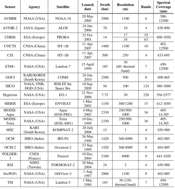
Figure 1: Measured extraterrestrial solar spectral irradiance at mean Earth-Sun distance.
Plotted from data in [3]. ... 4
Figure 2: Contributions to the remotely sensed signal. (a) Light scattered by atmosphere. (b) Specular reflection of direct sunlight at the sea surface. (c) Water leaving radiance. ... 5
Figure 3: Definition of the polar angles and of the upward (Ξu) and downward (Ξd) hemispheres.
ˆ
represents the versor identifying a direction determined by the angles θ and
. ... 6Figure 4: Surface radiance definition. ... 7
Figure 5: Measurement of the spectral radiance emitted by an extended horizontal source. . 8
Figure 6:Scheme of a MLP neural network. ... 23
Figure 7: Scheme of a RBF neural network. ... 24
Figure 8: (a) Example of Takagi-Sugeno rules. (b) Equivalent ANFIS ... 26
Figure 9: Linear separable case. ... 27
Figure 10: Non separable case. Cost-oriented formulation. ... 28
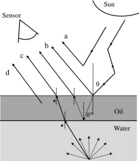
Figure 11: Contributions to radiance measured above an oil covered sea water surface. (a) Atmospheric path radiance. (b) Specular reflection of sky radiance. (c) Water leaving radiance. (d) Fluorescence and scattering contributions. ... 33
Figure 12: Scheme of the proposed oil spill detection system. ... 38
Figure 13: (a) An oil spill case from the dataset. (b) A look-alike case from the dataset. ... 41
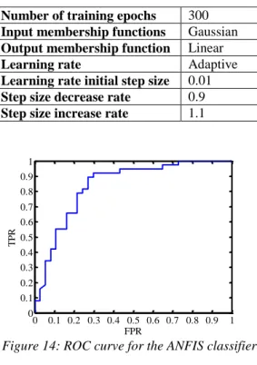
Figure 14: ROC curve for the ANFIS classifier. ... 46
Figure 15: Convex hull of three ROC curves. Lines α and β are two iso-performance lines, both tangent to the convex hull, but with different slopes, thus corresponding to different costs and class distributions. ... 49
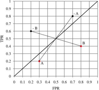
Figure 16: Classifiers A and B perform worse than the random classifier: by inverting their predictions we obtain classifiers -A and -B performing better than the random one. ... 50
Figure 17: Considering the predictions of classifiers 1 and 2, predictions of classifier 3 are swapped to obtain classifier 4. ... 51
Figure 18: Sliding window used for the online COID-SVM implementation. ... 52
Figure 19: Flowchart of the proposed approach for the classification based on an ensemble of online COID-SVMs. ... 53
Figure 20: ROC curves for the ensemble of online COID-SVMs. The violet curve represents the convex hull, whereas the black line represents the iso-performance line. The black squared mark is the optimum. ... 55
Figure 21: Time varying cost functions C(Y, n)(t) and C(N, p)(t), represented as a function of the online epoch number. ... 55
Figure 22: Effect of repairing convex hull concavities. ... 57 Figure 23: (a) Quickbird image (RGB) of the area of Castiglione della Pescaia (Grosseto, Italy), acquired on April 27th, 2007 at 10:32 UTC. The red square represents the bounding box enclosing the area covered by in-situ depth measurements, which are represented as
vii
have been acquired along two transects, represented as yellow and red dots, respectively. 61
Figure 24: Castiglione 2007 case: in-situ measured depth. ... 63
Figure 25: Castiglione 2007 case: mean STD obtained on the test sets as a function of the kernel dimension for the filter. In the plot the minimum STD, corresponding to the chosen kernel of 99 pixels, is highlighted by a black cross. ... 64
Figure 26: Experiment S-U: mean STD on training (blue dotted line) validation (red solid line) and test (green dashed line) sets for different number of clusters. The chosen number of clusters (32) corresponding to the minimum mean STD on the validation set is highlighted in the figure by a red circle. ... 66
Figure 27: Experiment S-U: scatter plot of depth estimated by ANFIS vs. in-situ measured depth for the training set (left) and for the validation set (right)... 67
Figure 28: Experiment S-U: scatter plot of depth estimated by ANFIS vs. in-situ measured depth for the test set (left). Estimated and in-situ measured depth for the validation set (respectively solid line and dashed line) along the transect dividing the considered bounding box in two (right). ... 67
Figure 29: Cumulative STD as a function of the absolute value of in-situ measured depth, obtained by ANFIS in the Castiglione 2007 case. ... 68
Figure 30: Path P1, black pixels are those belonging to the path... 69
Figure 31: Path P2, black pixels are those belonging to the path... 69
Figure 32: Path P3, black pixels are those belonging to the path... 70
Figure 33: Path P4, black pixels are those belonging to the path... 70
Figure 34: Experiment S-P3: scatter plot of depth estimated by ANFIS vs. in-situ measured depth for the training set (left) and for the validation set (right)... 72
Figure 35: Experiment S-P3: scatter plot of depth estimated by ANFIS vs. in-situ measured depth for the test set (left). Estimated and in-situ measured depth (respectively the solid line and the dashed line) along the transect dividing the considered bounding box in two and for the validation set (right). ... 72
Figure 36: Castiglione 2008 case: scatter plot of depth estimated by ANFIS vs. in-situ measured depth for the test set, that is Transect 1 (left). Estimated and in-situ measured depth (respectively the solid line and the dashed line) along Transect 1 (right). ... 74
viii
Table 1:Current Earth Observation multi-spectral and hyperspectral sensors. ... 2
Table 2:Current commercial Earth Observation satellites. ... 3
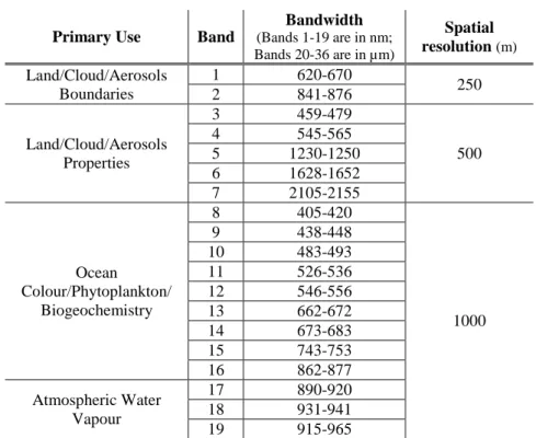
Table 3: MODIS specifications. ... 39
Table 4: MODIS bands and spatial resolution. ... 40
Table 5: Statistical parameters of the features calculated for oil spill cases in the dataset. . 43
Table 6: Statistical parameters of the features calculated for look-alike cases in the dataset. ... 43
Table 7: Classifier performances: the estimated relative error is 2%. ... 44
Table 8: Parameters for ANFIS training and architecture. ... 46
Table 9: Misclassification costs associated to each COID-SVM in the ensemble. ... 56
Table 10: Quickbird specifications. ... 60
Table 11: Quickbird multi-spectral bands ... 60
Table 12: STD obtained using the supervised method on the 2007 image where different median filters were applied ... 64
Table 13: Results of Experiments S-P1, S-P2, S-P3, S-P4. The errors obtained on each training set, on the test set and on the vertical transect are shown. The values are obtained by averaging results of multiple runs with the same configuration of ANFIS ... 71
ix
Symbol Definition
ANFIS Adaptive Network-based Fuzzy Inference System
AOPs Apparent Optical Properties
API American Petroleum Institute
AUC Area Under ROC Curve
CDOM Coloured Dissolved Organic Matter
EO Earth Observation
FPR False Positive Rate
GA Genetic Algorithm
IFOV Instantaneous Field Of View
IOPs Inherent Optical Properties
IR Infrared
LSE Least Square Estimate
MLP Multi Layer Perceptron
MODIS Moderate Resolution Imaging Spectroradiometer
MW Microwave
NIR Near Infrared
PCA Principal Component Analysis
RBF Radial Basis Function
REA Rapid Environmental Access
ROC Receiver Operating Characteristic
SAR Synthetic Aperture Radar
SG Specific Gravity
SLAR Side-Looking Airborne Radar
SVM Support Vector Machine
TOA Top Of Atmosphere
TPR True Positive Rate
UV Ultraviolet
Chapter One: Remote sensing of the marine environment: basic
concepts
1.1 Overview
Today, a wide variety of sensors, mounted on satellite platforms, is employed for Earth Observation (EO) activities, devoted to environmental monitoring. These sensors continuously acquire images of our planet, providing an extensive coverage across both space and time, and allowing the scientific remote sensing community to analyse a number of phenomena which may vary over large spatial and time scales. Since 70.9% of the Earth is covered by oceans [1], it is easy to understand that satellite images represent a powerful tool to study the marine environment. Among satellite sensors, we can distinguish between active sensors, such as radars, and passive sensors, such as spectrometers. The former are composed of an electromagnetic radiation source which emits directed energy pulses, and of a collector, which measures the backscattered signal. The returns from these radars, given by the reflection of active signals from small gravity and capillary waves, can be formed into images of the sea surface, that display a large variety of surface phenomena at a high resolution, and under nearly all weather conditions. The latter measure solar radiation reflected by the Earth surface, and the emitted blackbody radiation. Both day light and a cloudless sky are needed for these measurements. As will be explained later on, from the intensity and frequency distribution of the radiation collected by passive sensors we can study the ocean colour, which is used to retrieve information about sea water constituents, sea bottom properties, and the presence of polluting substances or anomalous algae growth. For this reason, in the present thesis only passive optical sensor data will be considered. The forerunner of ocean colour devoted satellite passive sensors was the Coastal Zone Colour Scanner (CZCS), launched by NASA in 1978. Since that date, a significant number of satellite sensors has been employed for studying the marine environment.
The importance given to EO missions can be understood by looking at Table 1 and Table 2, which list multi-spectral and hyper-spectral satellite sensors which are currently used for EO purposes by space agencies and by commercial satellite imagery providers.
Table 1:Current Earth Observation multi-spectral and hyperspectral sensors.
Sensor Agency Satellite Launch date Swath (km) Resolution (m) Bands Spectral Coverage (nm)
AVHRR NOAA (USA) NOAA-18 20 May
2005 2900 1100 6
580-12500
AVNIR-2 JAXA (Japan) ALOS 24 Jan.
2006 70 10 4 420-890
CHRIS ESA (Europe) PROBA 22 Oct.
2001 14
17 19
400-1050
34 63
COCTS CNSA (China) HY-1B 11 Apr. 2007 1400 1100 10 12500
402-CZI CNSA (China) HY-1B 11 Apr.
2007 500 250 4 433-695
ETM+ NASA (USA) Landsat-7 15 April
1999 183 30 (60- thermal band) 7 450-12500 GOCI KARI/KORDI
(South Korea) COMS
26 Jun.
2010 2500 500 8 400-865
HICO NASA, ONR, DOD (USA)
JEM-EF Int. Space Stn.
18 Sep.
2009 50 100 124 380-1000
Hyperion NASA (USA) EO-1 21 Nov.
2000 7.75 30 220 356-2577
MERIS ESA (Europe) ENVISAT 1 Mar.
2002 1150 300/1200 15 412-1050
MODIS-Aqua NASA (USA)
Aqua (EOS-PM1) 4 May 2002 2330 250/500/ 1000 36 405-14.385
MODIS-Terra NASA (USA)
Terra (EOS-AM1) 18 Dec. 1999 2330 250/500/ 1000 36 405-14.385 MSC KARI
(South Korea) KOMPSAT-2
28 July
2006 15 1 4 450-900
OCM ISRO (India) IRS-P4 26 May
1999 1420 360/4000 8 402-885
OCM-2 ISRO (India) Oceansat-2 23 Sep. 1999 1420 360/4000 8 404-885 POLDER-3 CNES (France) Parasol 18 Dec. 2004 2100 6000 9 443-1020 RSI NSPO (Taiwan) FORMOSAT-2 20 May 2004 24 2 4 450-900
SeaWiFs NASA (USA) OrbView-2 1 Aug
1997 2806 1100 8 402-885
TM NASA (USA) Landsat-5 1 Mar.
1984 183
30
(120-thermal band) 7
450-12500
Table 2:Current commercial Earth Observation satellites.
Satellite Company Launch Date Swath (km) Resolution (m) Bands Spectral Coverage (nm)
GeoEye-1 GeoEye 6 Sep. 2008 15.2 1.65 4 450-920
IKONOS GeoEye 24 Sep. 1999 11.3 3.2 4 445-853
Orbview-2 GeoEye 1 Aug 1997 2800-1500 1130-4500 8 402-888
Quickbird DigitalGlobe 18 Oct. 2001 16.5 2.4 4 450-900
SPOT-4 Spot Image 24 March 1998 60 20 4 500-1750
Worlview-2 DigitalGlobe 8 Oct. 2009 16.4 1.8 8 400-1040
1.2 Ocean colour remote sensing from optical sensors
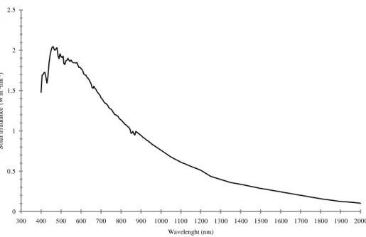
Optical sensors measure solar radiation backscattered from the sea surface at several selected wavelengths. As mentioned before, radiation sources for these sensors are the Sun and the Earth. In particular, the spectrum of the solar radiation (Figure 1) is close to that of a black body with a temperature of about 5800 K, thus, the Sun mostly emits in the visible and near-infrared part of the spectrum (0.4-0.7 μm) while the Earth, being at a mean surface temperature of about 280 K, emits mostly in the thermal infrared part of the spectrum (8-14 μm). Optical sensors for remote sensing of the ocean colour employ wavelengths in the visible and near- infrared, thus Earth emitted radiation can be considered as negligible. However, the photons from the sun can follow different pathways before they reach the sensor. In particular, we can consider the following main contributions to the remotely-sensed signal (see Figure 2):
- path radiance: light reaching the sensor after scattering of photons by the atmosphere;
- direct radiance: light reaching the sensor after specular reflection of direct sunlight at the sea surface;
- water leaving radiance: light upwelling from the sea surface after back-scattering in water.
In addition, we can note that light is also attenuated due to atmospheric absorption and scattering while going through the optical path from the source to the sensor.
It is only the upwelling water leaving radiance that carries any useful information on the water body, while atmospheric contribution and specular reflection at the sea surface represent noise sources, and must be corrected for. In particular, attenuation due to atmospheric absorption and scattering cannot be prevented during the remote measurement process, thus, the upwelling radiance from the water has to be processed by means of some atmospheric correction algorithm, in order to identify what the water leaving radiance contribution would have been if there were no atmosphere in between the sensor and the water body. Atmospheric correction represents an important issue for analytic approaches [2], since these algorithms need some initial estimate of many parameters characterizing
those atmospheric components which contribute to absorption and scattering of light. Such parameters must be determined using other sources of information, like in-situ measurements. However, for many cases these measurements could not be available.
Figure 1: Measured extraterrestrial solar spectral irradiance at mean Earth-Sun distance. Plotted from data in [3].
Looking in more detail at the water leaving radiance contribution, we can identify many factors affecting the signal. Direct sun light and diffuse sun light (that is sunlight scattered by the atmosphere) penetrating under the sea surface may be absorbed or scattered by water molecules, or by the various suspended and dissolved materials present in the water. Part of this light may reach the sea bottom (in shallow waters), and be reflected from it. At the end, part of the reflected radiation and part of the scattered radiation will reach the remote sensor. The remaining part will be scattered towards other directions, or it will be absorbed while going up.
Because of these processes, the signal collected by the remote sensor carries information on the type and concentration of substances present in water, together with bottom properties. In order to analyse the remotely sensed signal, it is important to understand how solar radiation interacts with the sea water body, and how the optical properties of sea water are modified by the presence of different types of marine constituents. In this framework, the effect of pure sea water, which is sea water in absence of any organic or inorganic matter other then water molecules and dissolved salts usually present in oceanic water, is usually distinguished from the effect of particulate, which can be classified into three main components [4] [5]: 0 0.5 1 1.5 2 2.5 300 400 500 600 700 800 900 1000 1100 1200 1300 1400 1500 1600 1700 1800 1900 2000 S o la r ir ra d ia n ce ( W m -2nm -1) Wavelenght (nm)
- Phytoplankton: the autotrophic component of plankton. They are able to carry out the photosynthetic process, thanks to the chlorophyll content within their cells. Other microscopic organisms are also included in this contribution.
- Suspended matter: suspended inorganic sediments.
- Yellow substance: coloured dissolved organic matter (CDOM). This contribution also includes detritus which have absorption characteristics similar to those of yellow substances.
In addition, we have to consider bottom contribution, which can influence the remotely sensed ocean colour in cases where the water is sufficiently clear and shallow. This contribution depends on depth, water transparency, and bottom type. The latter could be, for instance, sandy, rocky, coraline or algae covered.
Figure 2: Contributions to the remotely sensed signal. (a) Light scattered by atmosphere. (b) Specular reflection of direct sunlight at the sea surface. (c) Water leaving radiance.
Moreover, in the literature a distinction is usually made [6] [3] between Case 1 waters , which are those where phytoplankton contribution dominates and is the principal responsible for variations in water optical properties, and Case 2 waters, which are those waters where also suspended matter and yellow substance contribute.
The ocean colour is thus determined by scattering and absorption of visible light by pure water itself, as well as by the inorganic and organic, particulate and dissolved, material present in the water. The following paragraph reports a description of how these processes affect the remotely sensed signal.
Sun Sensor b a a a c Water
1.3 Ocean colour
The observed ocean colour is a direct consequence of the interaction of incident light flux with water molecules and with other organic and inorganic substances present in it. Spatial and time variations in water composition are then reflected in colour variations.
In order to interpret the ocean colour, it is useful to express the remotely detected signal as a function of concentrations of the various substances present in the water column. The following paragraphs define the link between radiometric quantities, which can be measured by remote sensors, and water constituent concentrations.
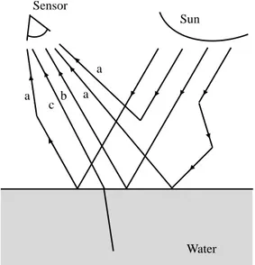
1.3.1 Radiometric quantities
1.3.1.1 GeometryFigure 3 shows the geometry of the problem. Polar spherical coordinates are used, so that a generic direction of light propagation, identified by a versor
ˆ, is expressed in terms of the zenith angle θ, between the direction of light propagation and the upward perpendicular to the horizontal reference plane, and the azimuth angle
, the angle between the vertical plane containing the light beam, and a specified vertical reference plane, usually chosen so as to simplify calculations. Here, according to the formulation used in [7] [8], the direction of zero azimuth is defined as the position of the sun.Figure 3: Definition of the polar angles and of the upward (Ξu) and downward (Ξd) hemispheres.
ˆ
represents the versor identifying a direction determined by the angles θand
.In Figure 3 the concept of solid angle is also represented: considering the area A on the surface of the sphere of radius r in figure, the solid angle, Ω, in units of steradians (sr), is the set of directions defining this area so that Ω = A/r2.
r Ξu Ξd ) , ( ˆ θ 1 ˆi 2 ˆi 3 ˆi A Ω
1.3.1.2 Radiant flux, radiance, irradiance
Radiant flux Φ can be defined as the radiant energy per unit time, Q/t, emitted by a point source (or by an infinitesimally small element of an extended source). Thus the radiant intensity is defined as:
t Q I (1)
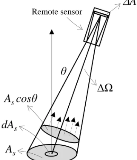
If we have an extended source it is necessary to consider the size of the area from which light is emitted or reflected. Radiance L is defined as the radiant intensity per unit area of a plane at right angles to the direction of light flow, L = dI/dA. Surface radiance is the radiant flux emitted in a given direction ξ = (θ,
) per unit solid angle, per unit projected source area. When the direction is not perpendicular to the source area As, the projected source area is Ascosθ (Figure 4). Field radiance at a point in space, in direction ξ, is the radiant flux in an element of solid angle dΩ, centred on ξ, passing through the infinitesimal area dA at right angles to ξ. The field radiance at a point in a plane surface surrounded by an infinitesimal area, dS, is the radiant flux through the projected surface area, dS cosθ. Spectral radiance, L(θ,
,λ) is radiance per unit wavelength, either passing a point in space (spectral field radiance) or emitted by an extended source (spectral surface radiance).Figure 4: Surface radiance definition.
An operational definition of spectral radiance is the following:
A t Q L , , (W m-2 sr-1 nm-1) (2)that is, the radiant energy Q measured over the integration time t, by a sensor with detector area A, angular field of view Ω, and bandwidth λ centred on λ. The measured spectral radiance is equivalent to the radiance emitted in the direction of the sensor by an extended source of area As, equal to the instantaneous field of view (IFOV), represented in grey in Figure 5. In particular, the radiant flux intercepted by the sensor is obtained by integrating the contributions of all infinitesimal area elements dAs, contained within the
r
)
,
(
ˆ
θ
A
Ω
IFOV, each contribution being proportional to the infinitesimal area times the cosine of the nadir viewing angle θ, whose variations within the area will be negligible for a sensor with a narrow angular field of view.
Figure 5: Measurement of the spectral radiance emitted by an extended horizontal source.
In order to measure L(λ) with a good resolution in all involved parameter domains, without encountering effects like diffraction, the intervals Δt, ΔA, ΔΩ and Δλ must be small enough. In practice, there is usually a tradeoff between the different parameters.
Using the definition of radiance we can also define the concept of irradiance. Plane irradiance is the total radiant flux per unit area incident on an infinitesimal element of a plane surface, divided by the area of that element and integrated with respect to solid angle:
L
d
E
,
,
cos
(W m-2 nm-1) (3)The cosθ term indicates that the contribution by radiance from different directions is weighted by the cosine of its zenith angle. When all directions are treated equally, we obtain the scalar irradiance, E0, that is the integral of the radiance distribution at a point over all directions about this point:
L
d
E
0
,
,
(W m-2 nm-1) (4)By integrating E over the upper and lower hemispheres we obtain the downwelling (plane) irradiance, Ed, and upwelling (plane) irradiance, Eu, which are the irradiances incident on a horizontal surface respectively from the upper hemisphere Ξd (where the light is travelling downward), and the lower hemisphere Ξu (where the light is travelling upward):
θ
A
sA
scosθ
A
Ω
dA
s Remote sensor
dd
L
E
d
,
,
cos
(W m-2 nm-1) (5a)
ud
L
E
u
,
,
cos
(W m-2 nm-1) (5b)Of course we can also define the upwelling and downwelling scalar irradiances:
dd
L
E
0d
,
,
(W m-2 nm-1) (6a)
ud
L
E
0u
,
,
(W m-2 nm-1) (6b)Downwelling and upwelling irradiances may be measured with a cosine collector, (angular field of view 180o) that measures the light falling on the surface of a flat diffuser, and is thus sensitive to light from different directions, in proportion to the cosine of the incidence angle. Thus, an operational definition of downward and upward spectral irradiance is the light incident on the detector area ΔA of a horizontal cosine collector, with spectral bandwidth of Δλ, over the integration time Δt, and pointing, respectively, downward or upward:
A t Q Ed d (W m -2 nm-1) (7a)
A t Q Eu u (W m-2 nm-1) (7b)Alternatively, downwelling irradiance may be measured using a Lambertian reference panel, that is. a panel with a surface which reflects radiance equally in all directions regardless of incidence angle. The radiance distribution reflected into the upper hemisphere from an ideal Lambertian panel would thus be isotropic. After correction for panel reflectivity, the downwelling irradiance may be obtained by multiplying the radiance reflected from the panel by π (this arises from the definition of irradiance in equation (5a)).
Regarding total scalar irradiance, measurements can be performed by recording the light incident on the surface of a diffusing sphere, which is equally sensitive to light from all directions, while upwelling and downwelling scalar irradiances may be recorded by shading the sphere from upper and lower hemisphere light, respectively.
1.3.1.3 Average cosines
A simpler way of specifying the angular structure of the light field is by determining its average cosines. The average cosine for the total light field is equal to the net downward plane irradiance divided by the scalar irradiance:
0E
E
E
d
u
(8)The downwelling average cosine and the upwelling average cosine, are respectively defined as
0E
E
d d
(9a)
0 E Eu u (9b)1.3.2 Apparent Optical Properties
Apparent optical properties (AOPs) are those optical properties of the water body which are influenced by the angular distribution of the light field, as well as by the types and concentrations of substances present in the water [9]. These properties are obtained from measurements of radiance or irradiance. In addition to the AOPs, inherent optical properties (IOPs) have also been defined [9]. These are independent of the angular distribution of the light field, and are determined exclusively by the properties of the water body, that are the types and concentrations of water constituents. The main AOPs used in remote sensing of the oceans will now be introduced, while IOPs will be discussed in Section 1.3.3.
1.3.2.1 Reflectance, remote sensing reflectance
For ocean remote sensing applications, reflectance is defined as the ratio between the upwelling and downwelling irradiances at a certain depth z:
, , , z E z E z R d u (10)For measurements taken above the sea surface, it is commonly used the spectral remote sensing reflectance, Rrs, defined as the ratio between upwelling, directional spectral radiance and downwelling plane irradiance:
, , , , , z E z L z R d rs (sr -1) (11)computed either immediately above the sea surface, z=0+ [10] or immediately below the surface, z=0− [7] [8]. The remote sensing reflectance is a measure of how much of the downwelling light that is incident onto the water surface is eventually returned through the surface, in direction (θ, ϕ), so that it can be detected by a radiometer pointed in the opposite direction.
1.3.2.2 Diffuse attenuation coefficient
Diffuse attenuation coefficient for downwelling irradiance (Kd) defines the rate of decrease of downwelling irradiance with depth:
K
dz z E z dE d d d
, , . (12)By integrating both sides of equation (12) we obtain the following:
K
z E z E d i d d , ln (13) whereE
E
d
z
0
,
i d , that is:
i
K
z d dz
E
e
dE
,
(14)thus, attenuation of light travelling in the water body from depth 0 to depth z follows an exponential law. This is actually true for a generic homogeneous medium, and is the basis for radiative transfer theory in atmosphere and in water.
Besides the diffuse attenuation coefficient for downwelling irradiance, the diffuse attenuation coefficient for upwelling irradiance (Ku) and for scalar irradiance (K0) can
analogously be defined. These coefficients are strongly correlated to the inherent optical properties of the water and also to other AOPs, such as reflectance.
1.3.3 Inherent Optical Properties
As anticipated in Section 1.3.2, inherent optical properties (IOPs) are determined by the types and concentrations of water constituents, and are not influenced by the angular distribution of the incident radiation field. The principal responsible for the fate of radiation entering the water body, and thus for the ocean colour, are absorption and scattering processes, that are described by means of some IOPs. Absorption removes photons from the light beam. These photons bring the absorbing molecules to higher energy levels. Scattering, on the other hand, make photons change their direction when impinging on molecules. In particular, we can distinguish between elastic scattering, which happens when the scattered photon has the same wavelength as the incident one, and inelastic scattering, which implies a change in the wavelength of the scattered photon. Among inelastic processes, we can mention Raman scattering by water molecules and induced fluorescence emission from CDOM and phytoplankton.
Considering natural sunlight in the visible part of the spectrum (roughly between 400 nm and 700 nm) as the only radiation incident on the water surface, the colour of the ocean is determined by scattering and absorption processes. In this context, the IOPs of relevance are the absorption coefficient (a, dimensions of [m-1]), which determines the exponential rate of decay of flux per unit pathlength of light in the medium, and per unit incident flux, due to absorption, and the scattering coefficient (b, dimensions of [m-1]), which defines,
analogously, the rate of decay of the flux due to scattering. In particular, scattering coefficients for elastic and inelastic processes must be defined separately.
It is important to note that both absorption and scattering coefficients are defined for a collimated, monochromatic flux, incident normally on the medium, and passing through an infinitesimally thin layer of the medium. They are not determined for natural conditions of illumination, as apparent optical properties are. Since AOPs, like reflectance, are usually measured using flat plate collectors facing downwards and upwards, with the angular distribution of the incident flux on the collectors being determined by environmental conditions, the relationships between inherent and apparent optical properties typically depend on the angular distribution of the light field under which apparent properties are measured. Hence, when linking IOPs and AOPs it is usually necessary to have a description of the angular distribution of the light field, which can be given by downwelling average cosine and upwelling average cosine, defined in (9a), (9b).
Because IOPs are not influenced by illumination conditions, they also have the advantage of being additive. More precisely, in a complex medium, composed of many different constituents, the contributions of individual constituents to an IOP can be summed together. This property is not valid for AOPs. Thus, scattering and absorption coefficients due to phytoplankton, CDOM, yellow substance and pure water are summed to obtain the absorption and scattering coefficients of Case 1 and Case 2 waters.
In Case 1 waters the dominant contribution is due to phytoplankton, so that other contributions co-vary with phytoplankton. Case 2 waters are more complex, and different contributions must be considered separately.
In particular, the contributions of each component to an IOP can be expressed in terms of the specific IOP of each component, that is, the IOPs per unit concentration of the component. Hence, the total absorption coefficient can be expressed as the product of the concentration of each substance and a corresponding specific absorption coefficient:
* * * s y p w P a Y a S a a a (m-1) (15)
where aw is pure sea water absorption coefficient, a , *p a and *y a are the specific *s
absorption coefficients for phytoplankton, yellow substances and suspended matter (in units of m2/g), and P, Y, S are the corresponding component concentrations (in units of g/m3). Backscattering coefficient can be treated analogously, assuming that yellow substances, being dissolved, do not contribute significantly to scattering:
* * bs bp bw b b P b S b b (m-1) (16)
The above relations allow to link the inherent optical properties of natural sea water to the concentrations of its constituents.
1.3.4 Relation between ocean colour and IOPs
Remote sensing measurements of the sea surface consist in a set of radiance or reflectance values which represent the apparent optical properties of the water body, and which also include the effect of light passing through the atmosphere. The number of available radiances or reflectances depends on the number of spectral bands of the sensor.
Ocean colour algorithms transform the set of radiances/reflectances into the values of constituent concentrations. In shallow waters the bottom effect must be also considered, thus water depth and bottom type represent additional unknowns.
Modelling the ocean colour means finding the relation between ocean colour and IOPs, and this implies that two issues must be faced:
- developing theoretical models which represent reflectance as a function of the specific IOPs;
- classifying the spectral behaviour of the specific IOPs of water constituents, also considering variability in water composition.
These issues make analytic modelling a difficult task. The following chapter describes possible approaches to the study of the remotely sensed ocean colour.
Chapter Two: Information extraction methods for remotely sensed
images
The study of the ocean colour can be used to retrieve concentrations of sea water constituents, water depth, bottom properties, or to detect pollutants. Many efforts have been made to develop techniques for information extraction from the remotely sensed ocean colour signal. However, without regard to the particular application, we can distinguish between two big branches of techniques: those relying on a Bayesian modelling approach, and those exploiting computational intelligence. The former try to develop a theoretical model of the water body under examination, and necessarily need to make some hypothesis on water composition, bottom effect, and atmosphere composition. Depending on the target quantity to be retrieved, also some measurements are needed. The number of these measurements depends on the water type (Case 1 or Case 2) and on the number of available bands. The latter do not make any hypothesis, but they use significant datasets of measurements of target quantities to be retrieved. When such a dataset is not available, simulated data can be used, exploiting some theoretical bio-optical models. In this case, the resulting approach will be a mixture of model-based and computational intelligence-based approaches.
2.1 Analytical methods
The simplest approach for retrieving water optical properties and/or water column depth from multi-spectral data is represented by regression methods, which derive the unknown properties from a number of measurements taken on site. These are called empirical methods, and their results are limited to specific case studies. More precisely, empirically derived relationships are valid only for data having statistical properties identical to those of the data set used for the determination of coefficients. These algorithms are thus particularly sensitive to changes in the composition of water constituents.
Model-based approaches aim to determine the relationship between the inherent and apparent optical properties of the water column. Among model-based approaches, we can distinguish between analytical modelling and radiative transfer modelling. Radiative transfer numerical models (e.g., Hydrolight [10] [11]) compute radiance distributions and related quantities (irradiances, reflectances, diffuse attenuation functions, etc.) in the water column as a function of the water absorption and scattering properties, the sky and air-water interface conditions, and the bottom boundary conditions. An analytical model is a simplification of the full radiative transfer equations, based on a set of given assumptions. Analytical models have the advantage that, due to their relative simplicity, they can be solved quickly. This is important in remote sensing applications, where a model must be evaluated at every pixel of an image.
If an analytical approach is followed, there are two ways to find the desired optical properties. The first one is represented by semi-empirical methods, which give direct or explicit estimates of target quantities. The second one is represented by implicit methods based on nonlinear optimization, which minimize the difference between calculated and
measured reflectance by varying input variables. Calculated radiance can be obtained either by means of analytical models (semi-empirical models) or radiative transfer models.
2.1.1 Semi-empirical methods
Semi-empirical methods use analytic expressions to relate apparent optical properties and water properties. In particular, two steps are followed: first an ocean colour semi-analytical model is implemented, then algebraic expressions are derived that relate ocean colour to the target quantities to be retrieved. A semi-analytical model is built using empirical data of the inherent optical properties, and of the concentrations of individual water components. Starting from these data, expressions relating optical properties and water components are derived, and a theoretical model is obtained. The model is then simplified, to reduce the number of unknowns, making use of approximations, or of the inter-dependencies between unknowns. The result is a set of algebraic equations that can be solved sequentially, starting from remotely sensed apparent optical properties, to obtain each of the unknown components of the model [5]. Examples of this approach can be found in [12] [13] [14]. If relationships are nonlinear, solutions may be found either by using look-up tables (in which results from multiple runs of the theoretical model are stored) or by means of bisection methods for reducing differences between predictions and observations.
The advantage of this approach is that it makes use of the known optical properties for specific components, and couples them with theoretical models of remote sensing reflectance. Although there are errors associated with the measurements used in the empirical relationships, the results appear quite accurate when applied to specific cases [12] [13]. Moreover, as stated before, these methods allow to quickly find the solution. On the other hand, one of the disadvantages is caused by the fact that empirical relationships, derived from measured data, tune the model to the specific regions where measurements have been taken. In other words, this approach gives accurate results when applied to specific cases, but has a limited generalization capability when the estimate is extended to different regions. Moreover, such methods can be implemented only with a limited number of unknown model parameters and variables (e.g. concentrations to be retrieved).
2.1.2 Implicit methods
A more refined approach with respect to semi-empirical methods is represented by the inversion of remotely sensed radiances, based on nonlinear optimization. In particular, a forward model for radiances at water level (which is usually a semi-analytical model) is inverted by minimizing the differences between the calculated values and the measured radiances. In particular, measured radiances undergo an atmospheric correction procedure, in order to be compared to calculated radiance at water level. The minimization can be performed using many different methods, but the basic concept which guides all these techniques is the search for the minimum difference between two spectral curves: the theoretical radiance and the remotely sensed radiance. More precisely, the χ2 of difference between modelled and measured radiances is minimized by iteratively changing the input parameters for the forward model. The χ2 is defined as:
22
Lsat Lmodel
χ (17)
where Lsat represents radiance measured from satellite sensor at water level, Lmodel represents theoretical radiance obtained by the model, and the sum is taken over all wavelengths λ. In particular, theoretical radiance can also be obtained by means of radiative transfer calculations, which, however, require a substantial computation time. A certain threshold is usually set to terminate the iterative minimization procedure. The input set of variables corresponding to the minimum represents the desired solution. Thus, water and bottom properties are simultaneously retrieved.
Nonlinear optimization techniques, together with model-based approaches have been widely used for ocean colour applications. In particular, analytical model inversions have been applied to the retrieval of water quality variables from airborne hyperspectral imagery [15] [16]. In [17] five water column and bottom properties (chlorophyll, dissolved organic matter, and suspended sediments concentrations, bottom depth, and bottom albedo) have been estimated by means of a Levenberg-Marquardt optimization method, using a remote sensing reflectance airborne hyperspectral dataset. In [18] a matrix inversion method has been used to retrieve water component concentrations.
These implicit methods are capable of reproducing the nonlinear nature of the modelled environment, and, once a forward model is adopted, they do not need any in-situ measured data. Most of implicit methods are based on a widely accepted model, proposed by Sathyendranath, Prieur, and Morel in [19], where sub-surface spectral reflectance is expressed in terms of absorption and backscattering coefficients. However, an underlying assumption of the optimisation methods is that the forward model is representative of the natural environment. This assumption, and thus the forward model choice, brings to a systematic error, which cannot be eliminated, nor it can easily be estimated. Generally speaking, all methods that are based on bio-optical models are affected by this systematic error. Other sources of errors are due to noise in satellite data, which however, unlike systematic errors due to model choice, appear in all methods.
Besides the disadvantage represented by systematic errors, several aspects of this techniques require attention during implementation. In particular, the parameterisation of the forward model should be carefully chosen, so as to ensure that the unknowns are as independent of each other as possible, otherwise ambiguities could arise in the estimation of desired quantities. An adequate selection of the initial guess is also of prime importance. This can be achieved by means of empirical algorithms, or by using the value from the adjacent pixel. Moreover, since multiple minima of the χ2 could bring multiple solutions, it is appropriate to set upper and lower limits for each quantity to be retrieved. This also contributes in reducing computation time, which however remains high.
Last, but not least, atmospheric correction represents an important issue, since estimates of many parameters, characterizing atmosphere composition, are needed in order to account for absorption and scattering of light, during the optical path between water level and sensor quote.
2.1.3 Principal component approach
All previously described approaches necessitate of an atmospheric correction to obtain water-leaving radiances. An alternative solution is represented by an integrated approach, in which the optical properties of the atmosphere are taken to be additional variables in an inversion problem [5]. Top of the atmosphere (TOA) radiances, measured by a satellite sensor, are the starting point for this inversion method. Target quantities are usually water component concentrations, bottom properties, as well as atmospheric parameters. Besides atmospheric correction, an additional issue to be considered is the high correlation between signals from different bands in Case 2 waters ocean colour data.
To address both issues, algorithms based on inverse modelling of the sea-atmosphere system through principal component multilinear regression, have been developed [20], in which the nonlinearity is managed by a piecewise-linear approximation. The main difference with respect to the previously described implicit methods is that the inverse model is not based on physical considerations: these are only used in the forward model, which is usually the one in [19]. The basic idea is to find a piecewise-linear map between a set of spectral TOA radiances and a set of geophysical quantities. In order to deal with the high correlation between signals from different wavebands, principal component analysis (PCA) can be exploited [21] [22]. Radiative transfer modelling is used to generate data sets of TOA radiances, corresponding to given variations of water constituents and atmospheric properties. Then, PCA of the simulated data is used to determine the spectral dimensionality of the data, and the weighting of each spectral channel required to retrieve the geophysical variables of interest. This approach accounts for the correlation between signals in different spectral channels, and improves reconstruction accuracy of retrieved constituents, giving better results than using subsets of the available wavebands. Principal components offer an orthogonal representation of the data, which allows the multivariate inversion, that would be hard to do with original radiances, due to high spectral correlation. A linear estimation formula is then derived to compute the geophysical variables from TOA measurements:
n j i j ij i k L A p 1 ˆ (18)where pˆ is an estimate of the target geophysical variable, j is the measurement channel i number, from 1 to n, where n is the number of spectral channels in the instrument, kij is the weighting coefficient of channel j for variable i, Lj is the measured radiance in channel j, and Ai is the offset value for variable i. By applying the method to TOA radiances, the atmospheric influence is implicitly taken into account. This approach relies on the fact that the application of an explicit atmospheric correction does not increase the information content with respect to water constituents and bottom properties. Although atmospheric scattering has a major influence on satellite data, these data also contain all signal variations caused by water constituents. Thus, signal variations that are not resolved in TOA data, cannot be resolved after atmospheric correction either.
The approach briefly described in this paragraph has the advantage of being a very simple, stable algorithm, which can be rapidly implemented even for large scenes, without
convergence problems typical of iterative inversion techniques. It also solves the problems related to high correlation and atmospheric correction. However, systematic uncertainty due to forward model choice still lasts. Moreover, the main limitation is due to the nonlinearity of the dependence between the optically significant substances and the radiances. To overcome these limitations computational intelligence techniques must be used.
2.2 Computational intelligence based methods
Computational intelligence techniques allow building a mapping from a set of input variables (e.g. TOA spectral radiance values, measured by a satellite sensor) to some output set of quantities (e.g. sea water parameter concentrations, bottom depth etc…). These techniques are able to represent nonlinear relationships between input and output quantities, and do not rely on any assumption or model choice. Not being affected by systematic errors, related to bio-optical models, computational intelligence techniques represent a valid alternative to model-based techniques. Moreover, the low computation time allow to easily process big remotely sensed images.
However, these are supervised techniques, therefore, a consistent dataset of input and target measured variables is needed to train an algorithm and build the mapping. The training dataset must be an exhaustive and representative set of the possible conditions the trained algorithm will be called to face in the application. Since in many cases such a dataset cannot be collected, simulated data, obtained by means of a forward theoretical model, are often used for training. For ocean colour applications the bio-optical model by Sathyendranath, Prieur, and Morel [19] is usually adopted.
Provided that a training dataset has been built in an appropriate way, and that overlearning has been avoided during the training phase, these techniques allow to achieve accurate results, and, more importantly, they have generalization capabilities.
The following paragraphs show some examples of computational intelligence techniques which have been used in the analysis of remotely sensed optical images, for applications in the retrieval of optically active constituents, or in the estimation of bottom properties and water depth.
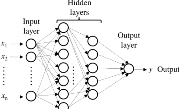
2.2.1 Neural networks
An artificial neural network is a parallel computing architecture that can be trained by supervised learning to perform nonlinear mappings. It can be regarded as a black-box model, which is able to represent the nonlinear relationships between input and output variables, any time a new input set is under examination, having learned from the examples which have been considered during the training phase. Such a network is made of a set of nodes, which are called neurons, eventually organized in layers, and connected together. Neurons represent the processing units of the neural network. The processing conducted by neurons consists in forming a weighted sum of the inputs, followed by a nonlinear transfer function to produce the output. The outputs of one layer become the inputs to the next layer in the network. Proper weights are established by supervised learning, using input data vectors with known desired outputs. Neural networks will be described in more detail in Section 3.1.