Improvement of a Genetic Algorithm for Manufacturing Optimization through Integration of Competence-based Criteria of the Working Personnel

F

I

RELAZIONE PER IL CONSEGUIMENTO DELLA LAUREA SPECIALISTICA IN INGEGNERIA MECCANICA

Improvement of a Genetic Algorithm for

Manufacturing Optimization through Integration of

Competence-based Criteria of the Working Personnel

RELATORI IL CANDIDATO

Prof. Ing. Gino Dini Daniele Marini

Dipartimento di Ingegneria Meccanica, Nucleare daniele.marini19@gmail.com

e della Produzione

Dipl.-Ing. Charlin Friederich

Institut für Fertigungstechnik und Werkzeugmaschinen Leibniz Universität Hannover

Sessione di Laurea del 10/12/2012 Anno Accademico 2011/2012

2

Abstract

Purpose: concept development and software modification to integrate worker´s

competencies into technological process chain optimization using mathematical models and a genetic algorithm.

Design/methodology/approach: A revision of GA applications found in literature is

necessary for select the right strategy to change the process models. The competences and knowledge theory for the personnel give a systematic way for collecting the workers skills and the needed competence to perform the job. The development of a new coefficient, the KOP, gives the possibility of having a parameter that connects the workers´ competencies with every process: this coefficient guides the planner to do a better worker assignment of the workers to the jobs, and obtaining process parameter influenced by the personnel. This is obtaining by the insertion of coefficients in the process models, taking in consideration the influence of the personnel on the process time (different for every kind of job). The modifications of the prototype develop a method which allows for an integrated technological and competence-based process chain planning. This method was implemented into a software prototype by programming a “competence-module”.

Findings: The changing of the process models gives as results of the GA a set of

parameters influenced by the competence of the personnel, and a set of KOPs optimally selected by the algorithm: the evaluation of the competence owned and needed bring to a production of another KOPs set. The systematic confrontation of these two sets, with the introduction of logic passages and a tolerance system, bring to an optimal selection of the personnel. The result of the validation shows an improvement of the performances, in relationship with the available pool of worker.

Originality/value: The proposed work can be considered as a first step to the

simultaneous and symbiotic optimization of the process parameters and the working personnel system. This is a first proposal to integrate the personnel in a systematic way, contemporary for the influence on time, cost, and parameters of the processes and for the assignation to the jobs themselves.

Keywords: personnel influence, competence based criteria, modified Genetic

Algorithms, personnel interacting GUI

3

Contents

1 INTRODUCTION ... 12

1.1 Thesis work procedure ... 13

2 THE GENETIC ALGORITHM ... 15

2.1 Introduction ... 15

2.2 The structure of the Algorithm ... 17

2.2.1 Chromosome representation ... 17

2.2.2 Selection mechanism ... 18

2.2.3 Evolutionary operators ... 20

2.2.4 Other Operators ... 22

2.2.5 Convergence Criteria ... 22

2.3 Single and Multi Criteria Optimization ... 23

2.3.1 Pareto Solution ... 24

2.4 Qualities and Flaws ... 25

3 THE MANUFACTURING OPTIMIZATION THROUGH THE GA ... 27

3.1 Introduction ... 27

3.2 Use of GA in Manufacturing Optimization ... 27

3.3 Forging process and forging die manufacturing... 45

3.3.1 Process chain planning ... 45

3.3.2 Process chain modeling ... 49

3.3.3 Process chain optimization ... 51

3.4 Analysis of the different GA application ... 56

4 COMPETENCE-BASED CRITERIA FOR THE WORKING PERSONNEL ... 58

4.1 Introduction ... 58

4.2 Competence of the Working Personnel. ... 58

4.2.1 Knowledge capturing ... 61

4.3 Developed Competences Assignation Method... 64

4.3.1 Personnel Skills ... 64

4.3.2 The Needed Competence ... 67

4.3.3 The assignment of jobs to the workers - Delta competence logic .. 69

4

5 DESCRIPTION OF THE PROTOTYPE ... 80

5.1 Introduction ... 80

5.2 The Database ... 81

5.3 The Genetic Algorithm ... 86

5.4 The Graphical User Interface ... 94

6 MODIFICATION OF THE PROTOTYPE ... 101

6.1 Introduction ... 101

6.2 Modification of the Database ... 102

6.3 Modification of the Genetic Algorithm ... 109

6.4 Modification of the Graphical User Interface ... 113

6.5 The new job assignment methodology ... 119

7 VALIDATION ... 125

7.1 Introduction ... 125

7.2 Description of the validation case: data settings ... 125

7.3 Validation results ... 132

8 OUTLOOK AND FURTHER DEVELOPMENTS ... 150

9 CONCLUSION ... 158

10 BIBLIOGRAPHY ... 161

11 APPENDIXES ... 163

11.1 Appendix A - Databases ... 163

11.2 Appendix B - GUI ... 165

5

List of figures

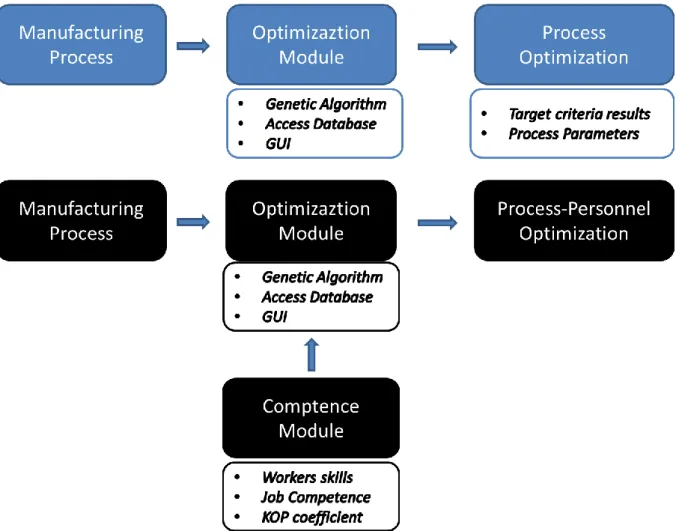
Figure 1.1: Procedures for the Prototype and the new Prototype with the competence

module 14

Figure 2.1: Procedure for a Genetic Algorithm 17

Figure 2.2: Scheme of the crossover single point 20

Figure 2.3: Scheme of a simple mutation. 21

Figure 2.4: Representation of a Pareto frontier 24

Figure 2.5: Summary of the GA optimization procedure. 26

Figure 3.1: Criteria used for the assignment of the workers to jobs 27

Figure 3.2: Scheme of the crossover single point 27

Figure 3.3: Scores of the ergonomic criteria for the job 29

Figure 3.4: Scores of the ergonomic criteria for the workers 30

Figure 3.5: Results ECRot. 30

Figure 3.6: An integrated framework of knowledge management 32

Figure 3.7: Knowledge based crossover 33

Figure 3.8: Flowchart of KBGA 34

Figure 3.9: Results of KBGA and comparison with SGA 35

Figure 3.10:The mPaGA chromosomes structure 36

Figure 3.11: Coefficient variations of mPaGA and tPaGA 36

Figure 3.12: Distribution planning for the supply chain 37

Figure 3.13: Decoding the combination and permutation states of the process route

for part I 38

Figure 3.14: A flow chart of the implemented modified genetic algorithm 39 Figure 3.15: One of the optimal manufacturing process plan for the modified genetic

algorithm 40

Figure 3.16: An overview of the proposed control-synthesis approach 40 Figure 3.17: Decision trees induced from traces of manual swing control 41 Figure 3.18: Fitness function for the genetic algorithm of the crane controller 42

6

Figure 3.20: Procedure of the reconstruct operation 44

Figure 3.21: Illustration of gasoline blending system 44

Figure 3.22: Quality and profit of products optimized with the DNA-HGA 45

Figure 3.23: Process chain model for forging processes 46

Figure 3.24: Sequence of the forging steps 47

Figure 3.25: Holistic dependency analysis of the processes and process chains 48

Figure 3.26: Relation of annealing temperature and hardness 50

Figure 3.27: Preference functions for the target criteria 52

Figure 3.28: Optimization results for different target criteria 54 Figure 3.29: Fitness values for best Pareto-efficient results 55 Figure 3.30: Distribution of the Pareto-efficient parameters 55 Figure 4.1: Competences' classification and sub-classification 60

Figure 4.2: Requirements of a knowledge base 61

Figure 4.3: Knowledge elements in the knowledge base 62

Figure 4.4: Technical skills of the worker 65

Figure 4.5: Individual skills of the worker 66

Figure 4.6: Individual skills of the worker 68

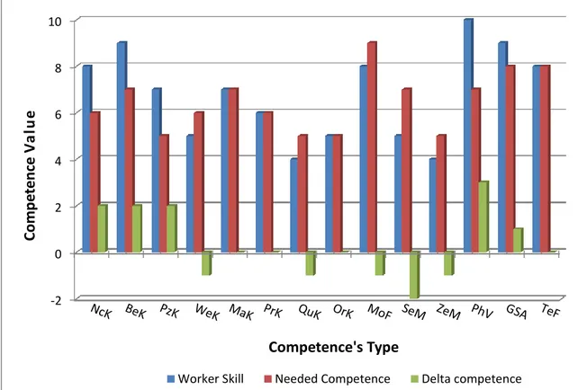
Figure 4.7: Personnel skills, needed competences and delta competences for the

combination worker nr. 2 and job nr.1 71

Figure 4.8: Procedure of the delta competences assignation 72

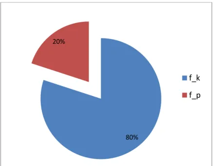
Figure 4.9: Percentage of influence of technical and physical competences for a fine

machining process 75

Figure 4.10: Percentage of influence of technical and physical competences for a

forging process 75

Figure 4.11: KOP components representation 76

Figure 4.12: KOP main elements representation 78

Figure 4.13: Visualization of the new GA optimization procedure. 79

Figure 5.1: Forging process chains 80

7

Figure 5.3: Access Database Relationships 82

Figure 5.4: Prozesskette table of the Access Database 84

Figure 5.5: Prozess table of the Access Database 85

Figure 5.6: Schematization of the connection present in the Database. 86 Figure 5.7: Direct process chain and indirect process chain alternatives'

Flowchart 87

Figure 5.8: FFs' folder of the prototype 88

Figure 5.9: Fine Turning Time FF elaboration 89

Figure 5.10: Fine Turning Cost FF elaboration 90

Figure 5.11 Fine Turning Quality FF elaboration 90

Figure 5.12: Composition of the direct and indirect chains combination 91 Figure 5.13: Total FFs of the GA for some case of direct and indirect chains 91

Figure 5.14: Schematization of the global FFs elaboration 92

Figure 5.15: Scripts of single-criteria GA optimization 93

Figure 5.16: Scripts of multi-criteria GA optimization 93

Figure 5.17: First page of the GUI 94

Figure 5.18: Popup page of the first page of the GUI for insert a new order 95

Figure 5.19: Second page of the GUI 96

Figure 5.20: Popup window of the second page of the GUI for insert a new process 97

Figure 5.21: Third page of the GUI 98

Figure 5.22: Popup page of the first page of the GUI for insert a new order 98

Figure 5.23: Fourth page of the GUI 99

Figure 5.24: Schematization of GUI-GA procedures' steps 99

Figure 5.24: Summarizing flowchart of the Prototype 100

Figure 6.1: Access relationships' table of the new Database 102 Figure 6.2: Schematization of the relationships in the new Database 102

Figure 6.3: Access Table of the Competences Needed 103

8

Figure 6.5: Access Table of the Personnel Skills (section two) 104

Figure 6.6: Access Table of the Process 105

Figure 6.7: Access Table of the Process-Personnel correlation (part one) 106 Figure 6.8: Access Table of the Process-Personnel correlation (part two) 106

Figure 6.9: Access Table of the Variables 107

Figure 6.10: Access Table of the Constants 108

Figure 6.11: New third page of the GUI 113

Figure 6.12: Popup window of the percentage of influence of the physical and

technical competence on the selected job 114

Figure 6.13: Popup window of the needed competences of the selected job 115 Figure 6.14: Popup window for the insertion of a new worker into the Database 115 Figure 6.15: Popup window of the competences and characteristics of the selected

worker 116

Figure 6.16: Job assignment flowchart 118

Figure 6.17: An example of job assignation 121

Figure 7.1: Schematization of the production system used in the validation: indirect

chain nr.1 and direct chain nr.4 123

Figure 7.2: Delta competences table for the skills of the experimental personnel and the need competences of the selected jobs in the Excel calculation file 131 Figure 7.3: Results Excel file for population 20, generation 50, KOP range v3.3

134 Figure 7.4: Graphical comparison for the oGA and nGA for Time FF value: population

20, generations 50, crossover 2 points 136

Figure 7.5: Graphical comparison for the oGA and nGA for Cost FF value: population

20, generations 50, crossover 2 points 137

Figure 7.6: Graphical comparison for the oGA and nGA for Time FF value: population

50, generations 50, crossover 2 points 137

Figure 7.7: Graphical comparison for the oGA and nGA for Cost FF value: population

20, generations 50, crossover 2 points 138

Figure 7.8: Graphical comparison for the oGA and nGA for Time FF value: population

50, generations 50, crossover arithmetical 138

Figure 7.9: Graphical comparison for the oGA and nGA for Cost FF value: population

9

Figure 7.10: Graphical comparison for the oGA and nGA for Time FF value:

population 100, generations 50, crossover 2 points 139

Figure 7.11: Graphical comparison for the oGA and nGA for Cost FF value:

population 100, generations 50, crossover 2 points 140

Figure 7.12: Graphical comparison for the oGA and nGA for Time FF value:

population 500, generations 100, crossover 2 points 140

Figure 7.13: Graphical comparison for the oGA and nGA for Cost FF value:

population 500, generations 100, crossover 2 points 141

Figure 7.14: Graphics of the GA for the case of 500 pop, 500 gen and KOP mode

142

Figure 7.15: Production Time results for the oGA and for the nGA in and

cases 145

Figure 7.15: Production Cost results for the oGA and for the nGA in and

cases 145

Figure 7.16: Workpiece Hardness results for the oGA and for the nGA in in and

cases 146

Figure 7.16: Workpiece heating temp. results for the oGA and for the nGA in in

and cases 146

Figure 7.17: Optimized KOP for the case of 500 pop, 500 gen and KOP mode r_v3.3 148 Figure 7.18: Personnel assignment results for the case of 500 pop, 500 gen and

KOP mode r_v3.3 148

Figure 7.19: Summary of the results of the nGA 149

Figure 8.1: Worker battery composition window. 151

Figure 8.2: Flowchart for the job assignment modified for the learning improvement

process 154

Figure 8.3: Learning option page for the GUI 155

Figure 8.4: Schematization of the model for the competence resistance FF. 156 Figure 8.5: Schematization of possible further developments. 157

10

Table directory

Table 3.1: Analysis of the different GA applications 57

Table 4.1: Example of workers' skills 67

Table 4.2: Example of needed competences for the jobs 69

Table 4.3: Example of workers' skills 76

Table 6.1: Changes in the FFs (part one) 109

Table 6.2: Changes in the FFs (part two) 110

Table 6.3: Changes in the FFs (part three) 111

Table 7.1: Needed competence for the jobs of the selected process chains 126 Table 7.2: Constants correspondent to the jobs of the selected process chains

128 Table 7.3: Worker skills for the selected personnel example 129 Table 7.4: KOPs for the experimental personnel for the selected process chains

131

Table 7.5: KOPs range for the validation tests 133

Table 7.6: FF values for the nGA and oGA. 143

Table 7.7: Process parameters results for nGA and oGA 143

Table 7.8: Target results for nGA and oGA 144

Table 7.9: KOPs optimization results for the validation test running 147 Table 9.1: Advantages and disadvantages of the new competence based

11

List of abbreviations

Symbol Description

GA

Gentic Algorithm

MSD

musculoskeletal disorder

ECRot

Ergonomic and Competent Rotation

FMS

Flexible Manufacturing System

SGA

simple genetic algorithm

KBGA

knowledge based genetic algorithm

CPU

central process unit

TP

throughput

MF

mean flow time

mPaGA

modified Pareto genetic algorithm

BOSC

build-to-order supply chain

tPaGA

traditional Pareto genetic algorithm

MPMLs

multiple parts manufacturing lines

DNA-HGA

DNA based hybrid GA

GUI

Graphical User Interface

FF

fitness function

nGA

new genetic algorithm

12

1

Introduction

The optimization of the industrial process is totally changed with the introduction of the calculator. In the past, after the construction of mathematical models, the optimization must be done through approximation method and simplification of the model by the experience of the planner: the reason is that the number of variables and of the complexity of the equations was hard obstacle. In the last years with the aid of a CPU other important steps could be done: the possibility of the use of the iteration, a massive number of operations could be done at the same time, with a speed unimaginable before. Some numerical method could be used for the approximation of some mathematical system, which constitutes the model of the industrial process that have to be optimized. The improvement of the computing power of the calculators conducts to another way: with the possibility of a lot calculations in a short time, the computer can be used not only in an instrumental way, but some methods are created almost only for a computational use. The genetic algorithm is one of these methods: through the simulation to the natural selection, the algorithm can select a prevailing solution of one function, also totally non-linear and with a huge number of variables, only with the variables' ranges where it would search the solution. Also more than one functions should be optimized: this kind of use of the algorithm brings to the reaching to a tradeoff solution, called Pareto efficient solution: the planner can select between more different optimal solution sets, and search the more comfortable solution for his case, with the consciousness of having the optimization all the variables for every set. The genetic algorithms use in the in industrial optimization has an impressive acceleration in the last 10-15 years: the development of software as MatLab and other software of numerical computing environments give the possibility to a largest scale application of this kind of programs.

Another major challenge for strategic human resource management research is establish a clear, coherent and consistent construct for organizational performance. The assignment of personnel to specific tasks constitute a crucial decision, since the very survival of the enterprise can depend upon an appropriate choice being made to optimize the assignment or selection process, there is a need

13

for some tool able to grasp all the complexity which vague information brings with it, as is also the case if the decision-maker is to reach a good solution. The simultaneous optimization of the process parameter and assignation of the workers becomes a target of all the manufacturing optimization process.

This work focus the attention of a particular case: an industrial forging line composes by two process chains that cross their selves in the forging operation. The process chains realize the production of the forged components and the forging dies, which have to be use in the production of the forged, manufacturing.

The process models and variables set are already developed: they are used for build the functions that the genetic algorithm uses for the optimization.

The data necessary for the optimization and for the selection of the alternative choices for the chains and the production system are stored into an Access Database. A prototype of a Graphical User Interface shows and permits to the planner to select the option of the chain, interact with the Database and run the algorithm.

The whole aim of the work is introduce the personnel influence into the results of the algorithm and find a way for realize a correct assignation to the workers, available to the planner, for every job.

1.1 Thesis work procedure

The work will begin with a general introduction on the genetic algorithm: after is developed an overview of various applications of the algorithm founded in literature, and the examination of the process models and the obtained results for the case in study and the old algorithm. The created competence-based criterion of the working personnel is showed in detail. After the description of the existing prototype in all this aspect and the modification that occur for apply the theoretic developed model and for reach the results. A necessary validation is the following step that would show the goodness of the work. A future development outlook concludes the whole thesis. A fundamental step is to find competence-based criteria for give a systematical evaluation to the working personnel, and decide how to connect the competence of the worker with the decision of personnel assignation to the jobs.The influence of the workers have to be induced to the optimization results: the only way is to modify the process models, so a modification into the Genetic Algorithm programming, with one

14

or more coefficients dependent to the workers' skills and to the needed competences for the job. The data of the personnel have to be stored into the Database for be used by the algorithm and also for a display into the Graphical User interface. The assignment of the workers to the jobs is a parallel problem: the best solution would be to find a way for make contemporary the optimization of the process parameters, taking in consideration the influence of the personnel on the system, and find the optimal battery of workers to assign to the jobs. The planner has to select the available workers' skills and the essential competences that the jobs need. The first aim of the whole work is obtain a set of process parameters influenced by the personnel, identifiable by the comparison with the old algorithm: with the possibly of demonstrate how the results of the optimization can improve with an optimal set of workers. The second aim is obtain the personnel battery that can realize the improvement of the optimal process parameters. The figure 1.1 shows a comparison between the prototype and the modified prototype procedure

15

2

The Genetic Algorithm

The Genetic Algorithms (GAs) is a heuristic search method, based on the imitation of the natural processes of evolution.

The GA, like the nature, works by evolutionary steps on a population of individuals, in order to obtain a state of a final population under specified rules: the evolution of population in nature is composed by two primary processes, the natural selection and the sexual reproduction. The first determines which members of population survive and reproduce, and the second ensures mixing and recombination among the genes of their offspring. In 1975, John H. Holland developed this idea in his book “Adaptation in natural and artificial systems”. He described how to apply the principles of natural evolution to optimization problems and built the first Genetic Algorithms.

The GA works at same for maximise the "fitness ", through the selection process of the variables and the evolutionary operators (i.e. mutation, crossover).

The population of GA is composed by single individuals called chromosomes or

strings.

For each generation the fitness of individuals is evaluated by a fitness function. This is the function that is necessary to maximize: the fitness function can be considered as the living organism. Evaluation of strings corresponds at the act of finding a solution of the function: the space, where the solution is searched depends by the fitness function itself.

All the individuals are composed by sub-units called genes: the position and the value of the genes determine the individual characteristics and proprieties, through encoding particular features: like the DNA makes for the living beings.

Usual the individuals are strings of bit, and consequently the genes are a number that can be 0 or 1; but also strings of real numbers can be performed by the algorithm (ref 2.2.1)

In each generation, the evolution operators modify the population. This is imitation of sexual reproduction is realized by the two operators: crossover, formed by merging

16

previous solution, and mutation, by modifying previous solutions. Crossover is a stochastic operator that allows exchange of characteristics between chromosomes (high probability). Mutation is an operator that flips some characteristics into a defined string (low probability). These operators will be examined in the following paragraphs. The selection statically screens and reduces, from the population, the individuals that have a relatively low fitness.

That procedure has stopped after a defined number of generations, or when the chosen termination ( or convergence) criteria (2.2.5).

The main parameters that the GA needs for implementation are:  J = population size

 = crossover rate  = mutation rate

The population size in usually considered between 50 units and 500 units: if the population should be too small, the GA will converge to a local minimum (for single criteria) or a Pareto minimum (for multi criteria). The concept of single and multi-criteria will be explained in subsection 2.3. Whether the population should be too large, the computational time will be so long.

The crossover rate is a probability, a number between 0 and 1, and gives the percentage of crossover among strings during a single generation: if this should be too small, the solution space will be too small, and this reduce the possibilities to find a local minimum. Whether it should be too large, algorithm will waste computational resources.

Also the mutation rate is a probability, and gives the percentage of mutation genes during a single generation: if this should be too small, many useful genes will never come out. Whether it is too large, we will have too many perturbations and the algorithm will lose his ability of use its history to improve.

Another not explicit parameter is important for the run of the GA: this parameter determines the initial seed that of population. For different initial population we will have really different results.

The only solution of this problem is repeat the running of the GA several times, for different values of the initial seed: through the evaluation of the best, worst and medium results, the different choices can be compared.

17

2.2 The structure of the Algorithm

The figure 2.1 shows a flowchart of the general procedure of a Genetic Algorithm.

Figure 2.1: Procedure for a Genetic Algorithm [1].

2.2.1 Chromosome representation

The representation of the chromosome consist into generate a string of binary or real numbers, in order to represent the variables of the problem, intended as the variables of the fitness function.

In the binary coding, the encoding of the variables of the problem to binary strings is function of the required precision and the length of the variables' domains. The necessary number of bits in the string is defined in the formula (2.1):

1 10 ) (

₂

2

x

x

Where, q is the required precision of variable xn, xnl and xnu lower and upper bounds of the domain of the generic variable xn, respectively.

18

The reverse process, obtain a variable from the binary string, is explained in the formula (2.2): ) ( ) (

2

x

x

x

x

Where decimal (substringn) is the decimal value of substringn relatively at variable xn. The main problem of binary coding is the not guarantee correlation between the problem space and the representation space: two points that are close in the problem space are not close enough in binary representation. Gray Coding is used for solve this problem. Gray coding convert a binary code vector, b = [b1, b2,…., bJ]T into a

Grey code vector g = [g1, g2, …, gJ]T, with the formula (2.3), and the reverse formula

(2.4):

g = Ab (2.3)

b = A-1g (2.4)

Where A and A-1 are the conversion matrices. In this way any two close numbers are different just for one bit: a single increase in the number value corresponds to a change of a single bit in the code.

Another problem of the binary coding is the request of length strings in order to represent high precision or large domain: with length strings occur problem of efficiency, due to the large representation space. The large number of bit into the strings create problem especially with a non-linear fitness function. Instead it’s possible to use a real coding. In the real coding each vector is composed by real numbers with the same length of the solution vector. In this way is possible to represent large domains, with a length more inferior than the binary.

2.2.2 Selection mechanism

The stage of selection chooses the individuals of the population for a later breeding (crossover or recombination). Selection is a method that randomly picks chromosomes out of the population, according to their evaluation function. A higher value of fitness function means a higher possibility of selection, according to Darwin's theory). The offspring will be the next generation, and selection drives the GA to improve the population fitness over the successive generations: the degree of the favouritism to the selection of the better individuals is called selection pressure.

19

Whether the selection pressure is too high, there is a premature converging to a sub-optimal solution. If it's too low, the GA needs a long time to find an sub-optimal solution. There are two groups of selection methods: proportionate selection and

ordinal-based selection. The first chooses the individuals basing on their relative values of

fitness function, the second picks up the individuals upon their ranking (ordering) within the population. Thus the selection pressure has to be independent of the fitness function, but only a dependence of the rank.

The most common fitness proportionate selection mechanism is the roulette-wheel

selection. The procedure can be summarized in these steps:

1. Calculate the fitness value eval (vj) for each chromosome vj eval (vj) = f (x) j = 1, 2,…..J were J = population size

2. Calculate the total fitness for the population:



v

3. Calculate the selection probability pk for each chromosome vj:

F eval

_v

p

4. Calculate the cumulative probability qj for each chromosome vj

_   J l l j p q 1 For the effective selection process:

1. Set j=1, were j is the number of the string 2. Generate a random number ρ [0, 1]

3. If ρ ≤ q1, select the first chromosome v1; otherwise, select the j-th chromosome

vj such that qj-1 ≤ ρ ≤ qj, where 2 ≤ j ≤J

4. Set j = j +1 and if j ≤ J go to step 2; otherwise, terminate the process of selection.

This method is really simple, only with J spins we can create a new population. Other relevant mechanisms are:

 Tournament Selection: population are divided in sub-groups and the best of the every subgroup is chosen for build the next generation.

 Reward-based selection: the probability of being selected is proportional to the cumulative reward obtained by the individual: this can be computed as a sum of the individual reward and the reward, inherited from parents.

20

 Ranking Selection: all the population receive a rank, the new population is created by the best ranking, without taking care the fitness function (linear ranking, exponential ranking,...)

2.2.3 Evolutionary operators

After the selection GA used two kinds of operator: crossover and mutation. Both are involved in the process of reproduction.

Crossover operator

Crossover is a stochastic operator that allows information exchanges between chromosomes. It's the most important genetic operator. A simple crossover can select at random in two strings, two cutting points and exchange the substrings generated by this process. The figure 2.2 shows a scheme of the crossover.

Figure 2.2: Scheme of a crossover single point.

The number of crossover in a generation is function of the crossover rate ( ).

The procedure of the simple crossover is the following:

1. the algorithm generates random number for every chromosome j: ; 2. if selects the j string for the crossover (minimum two);

21

3. it chooses a random integer : this indicates the position of the crossing point;

4. It keeps the left part of one parent and takes right of the other one, in this way two new chromosomes are generated for every couple.

If the number of chromosomes selected is odd, an extra chromosome can be added, or one chromosome can be deleted at random.

Other relevant crossover methods are:

 Crossover Two-Points or Three Points: more than one crossing point can be generating.

 Real number representation Arithmetical Crossover: the strings are composed by real numbers, the crossover among strings acts like a linear combination of vectors.

Mutation operator

Mutation operator produces spontaneous random changes into the strings, in order to introduce extra variability: the aim is to avoid a local minimum. A binary uniform

mutation can select one or more bits into a chromosome a flip the values of the bits

themselves. The figure 2.3 shows an example of uniform mutation.

Figure 2.3: Scheme of a simple mutation.

The number of crossover in a generation is function of the mutation rate ( )

The procedure of the binary uniform mutation is the following:

1. the algorithm generates random number for every bit of the population: ;

2. if selects the j bit for the mutation: 3. it chosen bits flip their values

22 Other relevant mutation methods are:

 Dynamic mutation: the number of changing bits is not a constant number, it is , where is variable in function of the position of the bit into the string and of the current generation.

 Real number uniform Mutation: the strings are composed by real numbers

xk, the mutation has a defined range of values for change them: the new value is xk’ = xkl + * (xku-xkl), where xkl is the low boundary limit, xku is the up boundary limit, and .

2.2.4 Other Operators

There are some kinds of other operators that act differently from the genetic. Some examples are shown following.

Niching: it involves the formation of distinct species exploiting different niches

(resources) in the environment. It can promote cooperative populations that work together to solve a problem. Whereas the simple GA is purely competitive, with the best individuals quickly taking over the population, niched GAs converge to a population of diverse species (niches) that together cover a set of resources or rewards [2].

Threshold: it is a parameter that must be exceeded or not in order to produce a

desired or undesirable effect: this can be used, for example, for control the diversity of population, which have to be over a threshold limit.

Reconstruction: two children are produced through the reconstruction. First, one

subsequence is cut from the rear of one parent, and then the cut subsequence is stuck at the front of another parent. Here the length of the cut subsequence is randomly selected. Second, another new segment with the same length of the cut subsequence is randomly generated and it will be stuck at the rear of the shorter parent. Third, the longer parent will be tailored to the predefined individual length L.

2.2.5 Convergence Criteria

The termination of the iteration of the algorithm is usually defined as the exceeding of certain number of generations T. Also the number of evaluation can be used like

23

termination criteria, especially when we have a lot of individuals that pass through without changing. These two criteria don't take care about the value of the fitness function, and also about the difference of fitness function's values in different generations: these criteria are connected only with computing time, and not with the accuracy of calculations. For consider this can be used a tolerance of variance of the

population's best fitness function value for a selected number of generations: the

genetic process will end if there is no change to the population’s best fitness for a specified number of generations. If the maximum number of generation has been reached before the specified number of generation with no changes has been reached, the process will end before. Instead of the population's best fitness value can be used the objective fitness function value.

2.3 Single and Multi Criteria Optimization

In the reality the great part of the problems of optimization doesn't concern only a single function, usually is multi-objective optimization problem.

In the single criteria optimization there is only one object- function (fitness function). A nonlinear problem for single criteria optimization can be formulated like as follow: Search x*= [x1*, x2*, ……xN*]T that satisfies:

 the K inequality constraints gk(x) ≥ 0 k = 1,2,….K

and M equality constraints hm(x) = 0 m = 1,2,….M < N

 minimize the objective function f(x) f(x*) = min f(x)

The vector will be x = [x1, x2, ….,xN]T is the vector of decision variables.

In the single criteria there is only one solution possible to the problem.

In multi criteria there are objective functions mutually conflicted: improving one of these fitness functions means to compromise the others.

Thus there is not a solution but a set of solution that is called Pareto Optimal set. The individuals in the solution are called non-dominated or not inferior.

24

2.3.1 Pareto Solution

The general formulation of a multi criteria optimization can be formulated like as follow:

search x*= [x1*, x2*, ……xN*]T that satisfies:

 the K inequality constraints gk(x) ≥ 0 k = 1,2,….K

and M equality constraints hm(x) = 0 m = 1,2,….M < N

 optimize the vector function f(x) = [f1(x), f2(x),…..,fI(x)]T where

The vector will be x = [x1, x2, ….,xN]T is the vector of decision variables.

The solution of the problem is a set, or frontier, of Pareto points that is the set of choices that are Pareto efficient. The Pareto frontier is particularly effectual in engineering: because with the choice among the different set of solution, there is the possibility a trade-off among these sets, and at the same time should consider all the range of the values. The solution to a multi-objective problem is a frontier of Pareto points that should be possible infinite. A design point in objective space

x

x

such that

_x

_x





_x

_x

j





j 1,2,...., . That is the dominance criterion. Then the Pareto frontier is the set of points from x that are not strictly dominated by another point in x.

In figure 2.4 there is an example of the Pareto set.

25

Between two different groups of Pareto solutions the best one is the group with

minus density of Pareto solution. Meanwhile for find the best Pareto solution into a

single group, especially when they are a lot, it's necessary a Coefficient Variation calculation of the obtained data.

2.4 Qualities and Flaws

In figure 2.5 is showed a summary of the optimization procedure. The qualities of GAs are the following.

1. Parallelism 2. Liability

3. Solution space is wider

4. The fitness landscape is complex 5. Easy to discover global optimum

6. The problem has multi objective function 7. Only uses function evaluations.

8. Easily modified for different problems. 9. Handles noisy functions well.

10. Handles large, poorly understood search spaces easily 11. Good for multi-modal problems Returns a suite of solutions.

12. Very robust to difficulties in the evaluation of the objective function.

13. They require no knowledge or gradient information about the response surface 14. Discontinuities present on the response surface have little effect on overall optimization performance

15. They are resistant to becoming trapped in local optima 16. They perform very well for large-scale optimization problems 17. Can be employed for a wide variety of optimization problems

The flaws are the following.

1. The problem of identifying fitness function 2. Definition of representation for the problem 3. Premature convergence occurs

26

4. The problem of choosing the various parameters like the size of the population, mutation rate, cross over rate, the selection method and its strength.

5. Cannot use gradients.

6. Cannot easily incorporate problem specific information 7. Not good at identifying local optima

8. No effective terminator.

9. Not effective for smooth uni-modal functions

10. Needs to be coupled with a local search technique. 11. Have trouble finding the exact global optimum

12. Require large number of response (fitness) function evaluations 13. Configuration is not straightforward.

Physical model Fitness Functions

GA

27

3

The Manufacturing Optimization through the GA

3.1 Introduction

The GAs are used for find the maximums or minimums of the functions: this can be used for all the process chain optimizations and for the optimization in general. After a representation through one or more function of the parameters that are object of the optimization, the fitness functions for optimization can be defined.

In this chapter some example of optimization find in literature are showed. After, the case of study will be examined: the process chains, the process models and the GA results.

3.2 Use of GA in Manufacturing Optimization

A genetic algorithm for the design of job rotation schedules considering ergonomic and competence criteria [5].

A genetic algorithm is used for generate a job rotation schedule in order to prevent musculoskeletal disorder (MSD), eliminate boredom and increase job satisfaction. Job rotation involves assigning employees to jobs that require different knowledge and skill levels: moving different muscle groups, decreases fatigue accumulation and consequently the potential for MSDs injuries. The design of efficient rotation schedules is a complex problem due to the many criteria: analysis of all these criteria will allow the design of operational rotation schedules, with the resulting health benefits for workers. Each job demands certain competences at different levels. Three kinds of criteria are used:

 ergonomic criteria;  physical skills required;  competence criteria.

All the criteria are in the figure 3.1, and all the values of the criteria for jobs and workers are showed in figure 3.2.The GA used is called “Ergonomic and Competent Rotation” (ECRot). The individuals are coded using a matrix of size × ,

28

being the number of participating workers (coinciding with the number of jobs in the rotation) and the number of rotations under consideration.

Figure 3.1: Criteria used for the assignment of the workers to jobs [4].

Figure 3.2: Scores of ergonomic and competence criteria for jobs and workers [4].

The ECRot have the following fitness function:

∑ ∑ Where:  ∑

29

 ∑

, competence fitness function.

With:

 , score of the ergonomic criteria j of the worker x in rotation r ;  , job assigned to the worker x in rotation r ;

 , score of the ergonomic criteria j of job ;  . duration of the rotation r ;

 , number of the ergonomic criteria;

 , number of the competence considered;

 , cost respect to competence j, of the worker x to job , in rotation r;  are constants dependent to and .

The ECRot run with an initial population of 50 individuals and 16 jobs assigned. Penalties are inflicted to the individuals that exceed the value (maximum time a worker is allowed to hold the same job post), the individual is penalized by increasing his fitness value. Crossover and mutation are applied to the matrixes.

For every worker and every job are selected the parameters of the criteria: figure 3.3 and figure 3.4 show the criteria's parameters of ergonomics criteria required for the job and owned by the workers.

30

Figure 3.4: Scores of the ergonomic criteria for the workers [4].

The value of the target function has a decreasing evolution, this is consequence of the elitist strategy employed for prevent disorientation. This advantage is counterbalance by the tendency to remain in the in specific zones, for these high coefficients of mutation and crossovers are used.

The figure 3.5 shows the results of the run of the ECRot.

Figure 3.5: Results ECRot [4].

The algorithm gives a suitable tool for the design of job rotation schedules which minimize the performance of time-extended and repeated body movements, diversify the tasks performed throughout the workday, and maximize worker performance by considering their competences for job assignment. In addition, the algorithm takes into account the workers’ physical disabilities, either temporary or permanent.

31

FMS scheduling with knowledge based genetic algorithm approach [5].

The GA solves a problem of scheduling of a Flexible Manufacturing System (FMS): this concern the definition of the resources and activity for maximizes the profitability, flexibility, productivity, and performance of a production system.

The FMS consists of three machine families (F1, F2, and F3), three load/unload stations (L1, L2, and L3), three automatic guided vehicles (A1, A2, A3): eleven different parts type are produced. Two performance measures are used: the throughput (TP) is the number of completed jobs during the scheduling period, the mean flow time (MF) is the flow times of jobs during the scheduling period. Due of this, the fitness function are:

 ∑  ∑ Where:

 , the number of part types;

 , flow time of ith part types ;  , arrival time of ith part types

 , completion time of ith part types

 , number of finished part of ith part types Also constraints have to be respected.

A segregated genetic algorithm (SGA) is used for solve the problem.

A Knowledge Management system is integrated: Knowledge management(KM) provides processes to capture a part of tactic knowledge through informal methods and pointers and fairly high percentage of explicit knowledge, reducing the loss of organizational knowledge (Nonaka & Takeuchi, 1995).

A framework of knowledge management is showed in figure 3.6: the conversion of the information to knowledge passes through various processes as verification, acquiring the filtered information, classification and creation of the knowledge from this information. After, the knowledge has to be distributed to the knowledge users.

32

Figure 3.6: Scores An integrated framework of knowledge management [5].

The integration of knowledge interacts directly with the GA: a knowledge based genetic algorithm (KBGA).

The knowledge is used not only for increase the performances of the system like a traditional genetic algorithm, also the performances of the algorithm are improved: the faster algorithm is developed by the use of the knowledge based initialization, knowledge based crossover, knowledge based mutation, and knowledge based selection.

 The knowledge initialization provides the initial population for the algorithm. Input information about the system environment like, machines, part, operation has been collected , after the performance measures have been decided, consequently the appropriate traditional scheduling rules has been selected and with this the seed of the initial population is created.

 The knowledge based selection is composed of three categories: o directional selection, based on the mean value of the population;

o steady selection, based on normalizing, eliminates the chromosomes with excessive values;

o unruly selection, eliminates the chromosomes according to the moderate values.

33

 The knowledge based crossover has the characteristics, performances and probability dependent on the knowledge base system: if any parent reproduce an unfeasible solution that is checked and eventually discarded. In figure 3.7 is showed a representation of this kind of crossover.

Figure 3.7: Knowledge based crossover [5].

 The knowledge based mutation used the knowledge base store for store the performances of the various mutation operators. Also the mutation probability is chosen according to the knowledge.

The flow chart of the KBGA is showed in figure 3.8.

One of the main aim is also minimize the number of generations: a less utilization of CPU time through a large combinatorial problem within a few number of generations. To evaluate the solutions' quality, the KBGA uses two performance measures: throughput (TP) and mean flow time (MF).

Maximization of throughput and minimization of the flow time are the aim of the algorithm: this means that is employed the maximum use of the resources within minimum time. The proposed KBGA maximizes the throughput with 5265.83units and minimizes the mean flow time with 1025.6 units.

34

Figure 3.8: Flowchart of KBGA [5].

A comparison study between simple GA and KBGA is showed in figure 3.9: in the table is showed the comparative results of the fitness functions' values and their standard deviations of KGBA, SGA and other scheduling strategies.

In the graphics are showed different characteristics that are evaluated for the number of generations: in the two graphics on the top are showed the convergence rates for KBGA and SGA (on the left), and the convergence of KBGA for different crossover probabilities, both for the TP performance criteria.

In the two graphics on the bottom are showed the same comparisons but for the MF performance criteria.

35

Figure 3.9: Results of KBGA and comparison with SGA [5].

The parameters of the GA vary with the environment, operating conditions and problem constraints. For this reason the algorithm is tested with a set of different crossover probabilities for both the performance measures.

Other examples of use GA's use in process planning

In this subsection for shortness are described other use of GA in other literature cases. Only the more relevant characteristics and main features are included.

A modified Pareto genetic algorithm for multi-objective build-to-order supply chain planning with product assembly [6].

A modified Pareto genetic algorithm (mPaGA) solves a problem of optimization of a build-to-order supply chain (BOSC). The BOSC includes supplier selection, product assembly and logistic distribution system that are integrated in this model.

36

 cost, including order cost, purchase cost and transport cost;

 delivery, maximum time of purchased parts transported to customer;  quality, the yield/throughput in the production system of supplier.

The constraints regard the equilibrium of supply and demand, the limit of production capacity and the flow equilibrium.

The variables are encode in strings like in the figure 3.10

Figure 3.10:The mPaGA chromosomes structure [6].

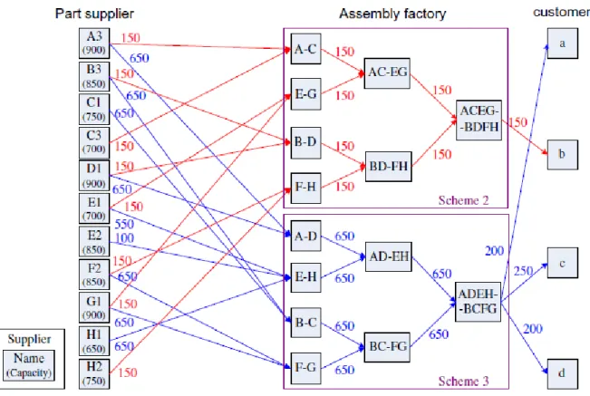
A niching operator is used before the reproduction process. After the crossover and the two stage mutation is used a equilibrium mechanism and a feasibility-adjustment mechanism that maintain the feasibility for each individual. In figure 3.12 is showed an example of distribution planning for the supply chain that is a solution of the optimization problem, obtained by the genetic algorithm. The distribution of different Pareto solutions is compared with a traditional Pareto Genetic Algorithm (tPaGA).

Figure 3.11: Coefficient variations of mPaGA and tPaGA [6].

In order to evaluate the best Pareto solution are compared different solution for both the genetic algorithms: the data obtained for Coefficients Variation are showed in

37

figure 3.11. In solving Pareto optimal solution the mPaGA has a smaller variation than tPaGA.

Figure 3.12: Distribution planning for the supply chain [6].

Modified genetic algorithms for manufacturing process planning in multiple parts manufacturing lines [7].

In this case the GA is used for decide a manufacturing process planning for a reconfigurable multiple parts manufacturing lines (MPMLs).

The representation scheme is a integer-base code: each string is composed of x segments, each segment represent a different combination of processing types available for the complete manufacture of a part. This means that if the production scenario is composed of a total of parts, then the process planning solution will contain strings, each string specifying the required processes for the manufacture of a particular part in the production scenario. In this application, the position of the gene location within the chromosome structure represents a processing identity (ID) composed of a specific stage, N, at which processing takes place by the selected processing machine, w: this is illustrated in figure 3.13.

38

Figure 3.13: Decoding the combination and permutation states of the process route for part i [7].

The decision value is specified in the third row. The experimental population of the GA contain a number of NC chromosomes really major than . A Cyclic crossover operation operates for each of the NC chromosomes in the population, the idea is to randomly select a chromosome. For each of the genes in a chromosome the idea is to randomly create a string for the ith part and then randomly exchange genes in the initial population. So the crossover operation changes the order between process machines in a string solution, without any violation of the constraints. The mutation changes randomly the bit in a string, also without violation of the constraints. A threshold operator imposes a limit for control the population diversity and prevents the premature convergence.

The necessary specific knowledge for generating manufacturing process plants includes: number of part families, part types and number of part types for each family to be processed, processes to be uses inclusive of alternatives, type of the machines, initial manufacturing configuration. In figure 3.14 is showed the flowchart of the GA.

The representing product information is:  part array;

 production volume array;  production cost array.

Representing manufacturing system information are:  process machine;

 part similarity coefficient;

39

Figure 3.14: A flow chart of the implemented modified genetic algorithm [7].

The two fitness functions regard:

 processing precedence relationships;  manufacturing capabilities limits.

In the figure 3.15 is showed a solution of the manufacturing process plan problem obtained by the algorithm.

A combined machine learning and genetic algorithm approach to controller design[8].

The study consists into a combination of machine learning and a GA optimization in learning to control a physical model of crane. Human control skills establish the control rules, and this knowledge is used by machine learning and then the GA improves the control performance with respect to the chosen criteria.

40

Figure 3.15: One of the optimal manufacturing process plan for the modified genetic algorithm [7].

For first, a GA is employed to learn control rules encoded as decision tables, without using prior knowledge about the controlled system. After, the learned rules are automatically transformed into symbolic machine learning. Finally, a GA is applied again, to optimize the numerical parameters of the induced rules. A flowchart of the logic applied is showed in figure 3.

Figure 3.16: An overview of the proposed control-synthesis approach [8].

For first, a GA is employed to learn control rules encoded as decision tables, without using prior knowledge about the controlled system. After the learned rules are automatically transformed into a symbolic machine learning. Finally, a GA is applied again, to optimize the numerical parameters of the induced rules. A flowchart of the logic applied is showed in figure 3.16. In crane control accurate positioning and appropriate swing control result have to be executed in the shortest time possible, taking into account the safety controls. The crane operates by control actions that are:

41  RIGHT-move the trolley to the right;  UP-move the load upwards;

 DOWN-move the load downwards;  STOP-stop current movement.

The task that have to be considered are: increasing swinging from zero to a specific amplitude, damping swinging under a specific amplitude. In figure 3.17 is represented the decision tree from manual swing control. The parameters of the control tasks are:

 time period ( )

 amplitude of load swinging (

 amplitude below the load swinging sets in swing-damping phase ( The control rules are dived in: State that denotes an attribute-valued vector consisting of the rope inclination and the related angular velocity ̇ ;and Action that is a user response to the current State, and represents a "class value'' for the learning program. Numerical values -1, 0 and 1 were used to denote classes LEFT, STOP and RIGHT, respectively.

42

The representation for the GA is an array of five components: the first two components represent thresholds for ̇ and in the swing-increasing rule, the remaining three components represented thresholds in the swing-damping rule, one for ̇ and two for . The range of searching for the ̇ thresholds was from ̇ 50°/s to 50°/s, and for from 10° to 10°.

For the fitness function is needed to define:

 crash: true, if the load hit the crane construction or the trolley hit the end of the track, otherwise is false

 time needed to carry out the experiment, (less than )

 number of the subtask that was under execution or finished at time (1 for

swing increasing, 2 for swing damping)  amplitude of load swinging at time , .

The fitness function that must to be maximize by the GA is showed in figure 3.18.

Figure 3.18: Fitness function for the genetic algorithm of the crane controller [8].

The results of the optimization are showed directly in the decision tree for swing control in figure 3.19.

Optimization of short-time gasoline blending scheduling problem with a DNA based hybrid genetic algorithm [9].

In this work a hybrid GA is used for an optimization of a gasoline blending process: the DNA based hybrid GA (DNA-HGA) is used to find a feasible region for a more accurate solution for running a Sequence Quadratic Programming (SQP) method searching.

43

Figure 3.19: Optimized decision trees for swing control [8].

The DNA-HGA uses a DNA encoding method: genes like nucleotide bases are used, so there are adenine (A), guanine (G), cytosine (C), and thymine (T), to represent the potential solutions of the optimization problem. They respond to the Watson–Crick complementary principle: A bonds with T, and G bonds with C. Integers 0, 1, 2, and 3 are adopted to encode the nucleotide bases, so the mapping from nucleotide bases to the digital integer is 0123/CGAT. Every variable is represented as an integer string of length l, one individual is L = n×l, where n is the number of the variable.

The genetic operators used are crossover, reconstruction (the figure 3.20 shows the reconstruction procedure for the DNA encoding chromosomes) and the mutation (three kinds of mutation: inverse-anticodon, maximum-minimum, normal).

In figure 3.21 is showed the gasoline blending system that have to be optimized: two kind of products are produced in the line, the regular gasoline and the premium. The fitness function that optimize the blending scheduling maximize the profitability of the products while satisfying the product quality and operating constraints. As operation restriction constraints are expressed by linear function, as specification of the product nonlinear constraints are given.

44

Figure 3.20: Procedure of the reconstruct operation [9].

Three cases are taking in consideration: recipes for one-day gasoline blending scheduling, recipes for three-day gasoline blending scheduling, recipes for one-day gasoline blending scheduling with uncertainly parameters.

Figure 3.21: Illustration of gasoline blending system [9].

In all the cases the cases the DNA-HGA gives better results than the normal GA, in the figure 3.22 is showed the results of the optimization for the profit and the quality.

45

After the GA an SQP method is used for alleviate the weak local search capability and increase the efficiency.

Figure 3.22: Quality and profit of products optimized with the DNA-HGA [9].

3.3 Forging process and forging die manufacturing

In this chapter is analyzed the case of study described in the article "Integrative

process chain optimization using a Genetic Algorithm" [1].

For first an overview about the two process chains: one for the component and another for the forging tool. The process models are showed as well as the use of the model for design the fitness functions. After the GA setting and the obtained results are displayed.

3.3.1 Process chain planning

A fundamental step where are analyzed the dependencies existent between the processes and also the process chains, concerning their importance for the defined target criteria.

The figure 3.23 represents a model of the forging process that shows the dependency between the processes of a same chain and between the processes of different chains. The forging die design and the forging manufacturing are optimizes simultaneously: the first one produces the die components for forging process that are used in the other chain for production of sleeves.

46

Figure 3.23: Process chain model for forging processes [1].

Three kinds of dependencies are considered:

 Within-process dependencies between the target criteria and the process parameters within one process,

 Process-process dependencies between two or more processes within one process chain,

 Global dependencies between the two process chains.

The first process chain acts the design and the manufacturing of the forging die, that consist in nine single components (figure 3.24) .

These components comprise a simple upper and lower die: in the main step of the forging process the upper die reflects a part of the model and the lower die ejects the manufactured part. The final step is a calibration of the workpiece.

The related die machining processes start with a roughing of the forging die, composed of an inner and outer turning. Another step of flat grinding is used in dependence of the manufactured piece. In order to set the hardness the die components are tempered in a vacuum furnace. In dependence to the requirements of the roughness the component is finally ground.

47

The process chain of the workpiece starts with the separation of the blank from the stock. This step is followed by an induction heating process for bring the piece to the forging temperature.

Figure 3.24: Sequence of the forging steps [1].

The third step is consequently a precision forging process with using a forging eccentric press. The following step is a cooling process where the temperature of the workpiece is bringing down to the ambient temperature by air cooling: into this project also the hardness of the piece is adjusted. The process chain ends with a turning process for inner and outer contours. For the optimization we have to consider the existent interdependencies

Therefore the dependencies, the influencing factors and the single target criteria have to be related with the single process. In figure 3.25 is showed a representation of the two process chains and an analysis of the process chains' parameters.

The chosen parameters that have to be respected, due to the large number of the dependencies and the optimization target are:

 forging die hardness, ;  workpiece temperature, .