Bancassurance : from organization to the wealth management and Armundia case

(1)

POLITECNICO DI MILANO

School of Industrial and Information Engineering

Master of Science in Management Engineering

Bancassurance: from the organization to the wealth

management and Armundia case

Relator: Prof. Laura Grassi

Correlator: Prof. Davide Lanfranchi

Author:

Mattia Dario Andreoli (878239)

(2)

Index of figures

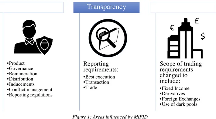
• Figure 1: Areas influenced by MiFID, page 7 • Figure 2: Sample of IDD test, page 9

• Figure 3: Standard IPID, page 10

• Figure 4: Global variation in financial literacy, page 12 • Figure 5: European variation in financial literacy, page 12 • Figure 6: Financial literacy among students, page 13 • Figure 7: Portfolio Selection, page 26

• Figure 8: Efficient portfolio, page 29 • Figure 9: Expected value of returns, page 30 • Figure 10: Set of possible combinations, page 31 • Figure 11: Set of possible combinations, page 33 • Figure 12: Expected value of returns, page 34 • Figure 13: Possible portfolio combinations, page 34 • Figure 14: Possible portfolio combinations, page 35 • Figure 15: Indifference curves, page 36

• Figure 16: Indifference curves, page 39

• Figure 17: Efficient frontier and risk-free security, page 40

• Figure 18: Life premiums and share distributed by banking, page 58 • Figure 19: Separate salesforce, page 59

• Figure 20: Hand in glove model, page 59 • Figure 21: Fully integrated model, page 59

• Figure 22: Strategical complementarity in bancassurance’s offer, page 61 • Figure 23: Strategical complementarity in bancassurance’s offer, page 61 • Figure 24: Types of relationship between banks and insurance, page 62 • Figure 25: Armundia Advisory360, page 63

• Figure 26: Financial coverage, page 64 • Figure 27: User view, page 65

(4)

Index of Tables

• Table 1: Sample of questions asked in a survey, page 16

• Table 2: N° of questionnaires that contains at least a question for each item, page 17 • Table 3: Average number of questions for each item, page 17

(5)

Sommario

Il seguente elaborato si propone di analizzare il contesto normativo in cui sti trova ad operare la bancassurance. Le direttive di riferimento analizzare sono MIFID II e IDD, le quali, nei recenti anni, hanno normato un panorama che prevede che i consumatori siano sempre più protetti e informati sui prodotti che intendono sottoscrivere. Dopo questa fase introduttiva, si procederà ad analizzare le modalità di gestione dei portafogli finanziari, valutando le tecniche utilizzate dai gestori per massimizzare il rendimento. Infine, verrà analizzato come avviene la distribuzione dei fondi una volta ricavati dal cliente. Successivamente, il focus verrà spostato sul ramo assicurativo ed in particolare si partirà ad analizzare prodotti più semplici, fino ad arrivare a quelli più complessi come assicurazioni unit-linked e index-linked. Prima di affrontare questi temi, ci sarà un breve excursus sulla matematica attuariale e la scomposizione del premio, al fine di capire la logica che si trova dietro questi prodotti. Come per la parte finanziaria, verrà spiegato come avviene il processo di distribuzione all’interno delle istituzioni assicurative. Nel quarto capitolo verrà introdotta la bancassicurazione nelle sue peculiarità, le sue forme organizzative e i canali distributivi. Dopodiché verrà introdotta la realtà di Armundia, piccola-media impresa che propone un servizio omnicomprensivo per supportare le realtà finanziare a svilupparsi e diventare bancassicurazione, grazie all’utilizzo di piattaforme IT che consentono di semplificare la vita degli operatori finanziari. Nel capitolo finale verranno riportate le conclusioni dell’elaborato.

(6)

Abstract

The following paper aims to analyze the regulatory context in which the bancassurance is operating. The reference directives to analyze are MIFID II and IDD, which, in recent years, have regulated a panorama that provides that consumers are increasingly protected and informed about the products they intend to subscribe to. After this introductory phase, we will proceed to analyze the financial portfolio management methods, evaluating the techniques used by the managers to maximize the yield. Then, it will be analyzed how the distribution of the funds takes place once they are obtained from the customer. Subsequently, the focus will be shifted to the insurance branch and in particular will start to analyze simpler products, up to the more complex ones such as unit-linked and index-linked insurance. Before addressing these issues, there will be a brief excursus on actuarial mathematics and the breakdown of the award, in order to understand the logic behind these products. As for the financial part, it will be explained how the distribution process takes place within insurance institutions. In the fourth chapter bancassurance will be introduced in its peculiarities, its organizational forms and distribution channels. Then the reality of Armundia, a small-medium enterprise that proposes a comprehensive service to support the financial realities to develop and become bancassurance, will be introduced, thanks to the use of IT platforms that allow to simplify the life of financial operators. The conclusions of the paper will be reported in the final chapter.

(7)

Chapter 1: MiFID and IDD, the customer as new focal point

1.1 MiFID II

MiFID II and the accompanying Regulation on Markets in Financial Instruments Regulation (MiFIR) are both pieces of legislation originating from the European Commission, seeking to provide a European-wide legislative framework for regulating the operation of financial markets in the EU.

MiFID II is concerned with the framework of trading venues and structures in which financial instruments are traded, whereas MiFIR focuses on regulating the operation of those trading venues, looking to processes, systems and governance measures adopted by market participants and to their future supervision.

The main impacts can be divided in three areas of interest and are:

In this document we will focus on the first section and how banks financial institutions intent to safeguard the customer. As said, the primary requirement of the MiFID II is to profile the investor to understand his degree of risk in order to structure for him the most suitable offer possible on the financial side1_.

1_{Cfr. art. 24 par. 2 e par. 3, MiFID II.}

•Product •Governance •Remuneration •Distribution •Inducements •Conflict management •Reporting regulations

Customer Protection

Reporting

requirements:

•Best execution •Transaction •Trade

Transparency

Scope of trading

requirements

changed to

include:

•Fixed Income •Derivatives •Foreign Exchanges •Use of dark pools

Market Infrastructure

(8)

The principal instrument adopted by banks and financial institutes is constituted by a survey. Currently this instrument is nothing more than a set of questions about the different knowledge and experiences in the financial world, as well as about personal economic situation and the possible returns to get from the investment. The banks then submit the “MiFID questionnaire” to the potential investor in the occasion of the investment proposal, whether they are online trading operations, or even the most common life insurance policies or any other instrument on the securities account. Differently from IDD survey, which will see further, the questionnaire is not standardized, but give a degree of freedom to the bank which provide it to the customer. What is equal for each test is the structure, that must report three main sections.

The principal points touched by the survey are 3:

1) Objectives of the investment: through simple questions, the customer is requested:

• Period of time through which it intends to keep a certain investment; • Risk appetite;

• The motivation that leads to investment;

• If it is a speculative investment or a real capital growth;

• If the customer invests to maintain and protect his capital avoiding loss, and if he is willing to accept certain levels of risk.

2) Financial situation: in this section, questions will be submitted concerning:

• Average customer earnings on an annual basis; • Primary source of income;

• Assets held;

• Any debts and credits.

3) Financial knowledge2_{: in this section all the data concerning the client are indicated and that}

has to do with the knowledge and experience gained in the financial field in the past. So, it's about:

• Knowledge of financial products; • Investment volume;

• Frequency; • Instruction; • Client profession

The MiFID questionnaire has the obligation, for banks and financial intermediaries, to assess the truthfulness and adequacy of the products or services that are offered to the potential new customer, based also on our knowledge. In this way an investor profile is outlined and this allows the bank or

(9)

the broker or the financial promoter to proceed in harmony with the client's knowledge of the most appropriate type of investment.

The structure of the survey can be summarized in this way:

In essence, the MiFID questionnaire gathers as much information as possible, to propose appropriate investment information for the trader or the customer.

Then, the promoter company that acquires the client's investments must act honestly, impartially and as professionally as possible, always trying to provide clear and very correct information, but above all relating to the investments required.

1.2 IDD

On the other side, as said before, we can focus on insurance distribution because, from October 2018, a new directive has been released: The Insurance Distribution Directive (IDD). As for the MiFID II, the IDD expressly states that EIOPA (main authority in terms of Insurance at European level) conducts consumer testing before finalising the draft ITS, now the standard in term of survey3_.

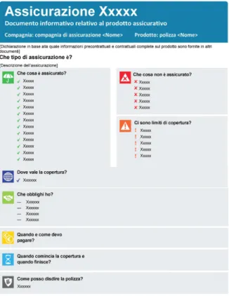
The test studied for the IDD is divided in different questions, necessary to understand the needs of the future customer. This test will help not only the client but even the contractor to understand in the correct profiling. One example that can help us understanding the utility of this test is in case of an offer: if the customer does not have the car, probably, in the omni comprehensive package will not appear an insurance against damages with car.

A sample of the test will be reported in the figure below:

3_{The reference point of this paragraph is the report “IPID Consumer Testing and Design Work” taken from}

the EIOPA internet site https://eiopa.europa.eu/and the work is collected with the name EIOPA/OP/153/2015

(10)

As ween can see, main questions are related to the need of being insured against car incidents or house-damages. This test, as said before, will provide information about the need of the client in order to carve the most suitable offer.

As soon as the result are available, the customer will be put in front of a paper which reports the most suitable offer. In facts, as well as ESMA (The European Securities and Markets Authority is a European Union financial regulatory institution and European Supervisory Authority, located in Paris), EIOPA set a presentation format of an Insurance Product Information Document (IPID) specifying the details of the presentation of the information. The insurance product information document, which will be prepared for non-life insurance products only, needs to contain the following information:

a) information about the type of insurance;

b) a summary of the insurance cover, including the main risks insured, the insured sum and, where applicable, the geographical scope and a summary of the excluded risks;

c) the means of payment of premiums and the duration of payments; d) main exclusions where claims cannot be made;

e) obligations at the start of the contract; f) obligations during the term of the contract; g) obligations in case of a claim made;

h) the term of the contract including start and end date of the contract; and, i) the means of terminating the contract.

(11)

The IPID will be supplied to the consumer by the insurance distributor prior to the purchase of a non-life insurance product with the goal of assisting the consumer to make an informed decision. As we can see, the IPID is divided in different parts which cover different aspects of the financial situation and the behaviour of the new customer. The IPID could be compared to the KIID, introduced by ESMA, but is more comprehensive because, if KIID is related just to UCITS funds4_,

this document must be provided for every insurance product.

This survey, as well as MiFID one, is focused on understand the financial literacy and providing the most suitable products to the clients.

1.3 Points of contact and Italian view

In this chapter we aim to provide an overview of the Italian situation with reference to the investment process and how the consultancy application fits into it. Therefore, some statistical data will be presented regarding the degree of financial literacy in our country and the attitudes of Italians with regard to investment choices - from which a concrete "need for advice" can be deduced - the issue of behavioural biases in which they may incur is addressed. Both investors and consultants, with particular reference to the perception of risk. Finally, investors' attitude towards consulting is described in terms of the variables considered in the professional's assessment. OCSE, in the investigation PISA5₂₀₁₅

The most important international statistical surveys on the level of financial literacy are PISA and the "Standard & Poor's Ratings Services Global Finiteness Survey"6_{. The results that emerge from}

the most recent editions of these publications do not give an excellent image of our country compared to the other industrialized countries. In particular, on the basis of the S&P survey, Italy is not at the top of the list, neither in the world nor in Europe, as can be seen from the following figures7_:

4_{UCITS - The Undertakings for the Collective Investment of Transferable Securities (UCITS) is a regulatory}

framework of the European Commission that creates a harmonized regime throughout Europe for the management, marketing and sale of mutual funds

5_{PISA, is the acronym of Programme for International Student Assessment, it is an international}

investigation promoted by the OCSE and it has the scope to evaluate the level of instruction among students within industrial countries.

6_{The S&P FinLit Survey is the most accurate investigation on the financial literacy held at an international}

level. In the edition of 2015, around 150.000 people have been interviewed in more than 140 countries. The four questions most asked refer to these important aspects: risk diversification, inflation,

numeracy(interest), compound interest

7_{Data and figures used are taken from the book: McGraw Hill Financial, Financial Literacy Around the}

(12)

In particular, financial literacy rates vary widely across the European Union (Map 29). On average, 52 percent of adults are financially literate, and the understanding of financial concepts is the highest in the northern Europe. Denmark, Germany, the Netherlands and Sweden have the highest literacy rates in European Union: at least 65 percent of their adults are literate in financial terms. But rates are much lower in southern Europe. For example, in Greece and Spain, literacy rates are 45 percent and 49 percent,

respectively. Italy and Portugal have some of the lowest literacy rates in the south. Financial literacy rates are also low among the countries that joined the EU in 2004 and after. In Bulgaria and Cyprus, 35 percent of adults are financially literate. Then Romania, with 22 percent has the lowest rate in European union.

Present data are referred just to adults. If we look even at young Italians, they rank slightly below the OECD average, placing Italy between seventh and ninth in the ranking of the 15 countries that

Figure 5: European variation in financial literacy Figure 4: Global variation in financial literacy

(13)

participated in the PISA financial literacy survey in 20158_{. On average, only 6.5% of Italian students}

reach the highest level (level 5) of performance on the PISA scale relative to financial knowledge9_.

Numerous studies show that a high level of financial literacy has positive repercussions both on an individual and macro-economic level.

Data reported have the purpose to demonstrate that in the Italian optics, not so much people have the right instruments to understand if the investment proposed is good or bad for their wealth. The need to have a survey where to communicate the intentions and the awareness of the customer may represent a way to protect the potential investor.

For this reason, one of the fundamental moments of the consultancy is notoriously that of assessing the adequacy of the investments subject to recommendation with respect to the risk profile and other personal characteristics of the investor.

In almost all cases, the collection of information by the customer is carried out by administering a standardized questionnaire, in which questions are asked to the client about his work situation, his financial situation to assess in particular his tolerance to suffer losses (objective risk), on their knowledge of the main financial concepts such as risk-return and diversification, and finally on his personal risk appetite (subjective risk). As mentioned, in the absence of such information the

8_{This part of the PISA’s survey, related to the financial literacy is not mandatory. In 2015, just 15 countries}

have joined this option, 10 of these are already members of OCSE (Australia, Belgium, Canada, Chile, Italy, Netherlands, Poland, Slovakia, Spain and USA). In addition to this, it just concerns a few numbers of students. In Italy, this sample refers just to 3.035 students, 2.724 with valid data, within a total of 11.583 students involved.

9_{Elaborations are taken from INVALSI document (Istituto nazionale per la valutazione del sistema}

educativo di istruzione e di formazione): “Indagine OCSE PISA 2015 - Financial literacy Sintesi dei risultati”. The reader can see this document to the following link:

http://www.invalsi.it/invalsi/ri/pisa2015/doc/2017/Sintesi_Financial_literacy_24052017.pdf

(14)

intermediary is prohibited from proceeding to provide the recommendation to the client, pursuant to art. 54 par. 8 of the MiFID II Delegated Regulation10_.

This because, on an individual level, people with more financial knowledge are supposed, among other things, to make better decisions about their financial wealth, to save more for their retirement, to manage their balance sheet better, to participate in stock markets, to operate more diversified portfolio choices and, ultimately, to choose investment funds with contained commissions. Not possessing financial notions and skills produces mirror-like results. Those who are financial "illiterate" usually save less and get more debt by paying higher fees and interest.

On a macro-economic level, the most literate people, demanding better quality services, stimulate competition and innovation. They are also able to better tolerate systemic financial shocks, are less likely to make irrational decisions, and therefore also allow governments to help and intervene in support of investors who have taken bad decisions.

One of the fundamental moments of the investment process is notoriously that of assessing the adequacy of the investments subject to recommendation with respect to the risk profile and other personal characteristics of the investor.

In almost all cases, the collection of information by the customer is carried out by administering the survey, object of our analysis, in which questions are asked to the customer about his work situation, his financial situation to assess in particular his tolerance to suffer losses (objective risk), on their knowledge of the main financial concepts such as risk-return and diversification, and finally on his personal risk appetite (subjective risk). As mentioned, in the absence of such information the intermediary is prohibited from proceeding to provide the recommendation to the client, pursuant to art. 54 par. 8 of the MiFID II Delegated Regulation.

It should also be remembered that financial consultants of any kind are required to issue, for each consultancy given, a suitability report that contains the details of the recommendation provided and the reasons why it was deemed adequate to the customer. As clarified by ESMA in a Questions & Answers dedicated11_{, among other things, to the assessment of adequacy, this report must be issued}

to the customer prior to the execution of the order, even if the investment is not followed by the recommendation and also when the recommendation consists of a advice not to buy (not to buy). The problem that one wants to put in relation to the use of the questionnaire is if it, as it is formulated today in the practice of each credit institution or investment firm, is really able to grasp the information that it aims to obtain from the customer. The empirical researches conducted on this aspect, although not numerous or recent, are in agreement in recognizing wide margins of

10_{Delegated regulation 2017/565/UE of April 2016}

(15)

improvement given the vulnerability of the questionnaire to the cognitive errors and to the behavioural distortions of the clients, of which it was widely discussed in the preceding pages. In particular, as emphasized by ESMA in its "Guidelines on some aspects of adequacy assessment"12_,

questions should be formulated to take into account the possible cognitive biases of investors and the questionnaire itself should be unbiased, that is, to contain questions in a way that makes the answers unreliable. Specifically, ESMA suggests to counterbalance self-assessment through objective criteria, such as for example: "a) instead of asking whether a client understands the notions of risk-return trade off and risk diversification, the firm could present some practical examples of situations that may occur in practice, for example by means of graphs or through positive and negative scenarios, asking to choose which one would be correct/real in his opinion; instead of asking a client whether he feels sufficiently experienced to invest in certain products, the firm could ask the client what types of products the client is familiar with and how recent and frequent his trading experience with them is; (c) instead of asking whether clients believe they have sufficient funds to invest, the firm could ask for factual information about the client’s financial situation; (d) instead of asking whether a client feels comfortable with taking risk, the firm could ask what level of loss over a given time period the client would be willing to accept, either on the individual investment or on the overall portfolio. "

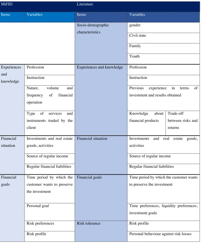
In a Consob discussion paper of 2012.251 dedicated to the evaluation of risk tolerance through the MiFID I questionnaires, the discrepancy between the indications of the behavioural finance literature and the indications of MiFID I was shown first. The authors also analysed a sample of 20 questionnaires, examining their contents, reliability, structure and methods of administration to customers. This information was collected through an interview prepared by Consob and administered to the intermediaries involved in the research.

The following tables summarize some evidence emerged in the research:

(16)

MiFID Literature

Items Variables Items Variables

Socio-demographic characteristics gender Civil state Family Youth Experiences and knowledge

Profession Experiences and knowledge Profession

Instruction Instruction

Nature, volume and

frequency of financial

operation

Previous experience in terms of investment and results obtained

Type of services and instruments traded by the client

Knowledge about

financial products

Trade-off

between risks and returns

Financial situation

Investments and real estate goods, activities

Financial situation Investments and real estate goods,

activities

Source of regular income Source of regular income

Regular financial liabilities Regular financial liabilities

Financial goals

Time period by which the customer wants to preserve the investment

Financial goals Time period by which the customer wants

to preserve the investment

Personal goal Time preferences, liquidity preferences,

investment goals

Risk preferences Risk tolerance Risk profile

Risk profile Personal behaviour against risk losses

(17)

Another interesting aspect emerging from the Consob reports concern the linguistic and textual profiles of the questions. "[...] Only two of the 20 questionnaires analyzed can be considered sufficiently clear, effective and "valid" because they use precise questions and uniquely identify the quantity to be measured; the remainder indistinctly detect an aptitude for risk, risk capacity, risk tolerance and investment objectives that are missing in lexical and comprehensibility terms ”13_.

The questions, particularly those concerning the familiarity to investments, are often double (barrelled) - they refer to several themes simultaneously and so they suggest the answer themselves. The formulation of the questions can also induce the subject to improve his image, knowingly or unknowingly, by providing false answers. Other potential customer biases are the unconscious tendency to respond positively to dichotomous questions (of the type yes, no), to position themselves centrally in the scales for questions involving alternatives arranged in scale (c.d. acquiescence or central tendency).

13_{N. Linciano e P. Soccorso, La rilevazione della tolleranza al rischio degli investitori attraverso il}

questionario, p. 45 0 5 10 15 20 25

Table 2: N° of questionnaires that contains at least a question for each item

0 1 2 3 4 Know ledge Natur e/ Vo lume Instru ction /Prot ectio n Sour ce of reve nues _Assets Inves tmen ts and … Finan cial lo ans Finan cial h orizo n Risk a dvers ity Risk p rofile Inves tmen t sco pe

(18)

Finally, the use of inaccurate terms that can give rise to misunderstandings or difficult to understand technical terms is noted.

In conclusion, I believe that the questionnaire is a suitable tool but that it can be improved by using the measures dictated by "behavioural finance". I also believe that, with regard to the method of administration, the way to go is to encourage the client to go personally to the intermediary and to complete the form with the help of the consultant. In such a way as to be able to respond comprehensively and completely to all the questions and to be guided, in a wise and completely disinterested manner, by an advisor.

(19)

Chapter 2: how to create a financial portfolio according to new

directives

As already analysed in the previous chapter, a customer can be classified based on objective criteria to which the intermediary will have to refer in order to associate to the new investor the most appropriate portfolio. In fact, after the process of data gathering, usually done with questionnaires, the customer will be defined as:

• Retail if it has low knowledge and experience in the field of investments. This category of investors is subject to strong protection by the MiFID regulation.

• Professional, In the event that the customer has significant knowledge and experience in the field of investments.

As a next step, the client is subjected to an appropriateness test. It represents a valid criterion for verifying that the investor has sufficient knowledge to understand the risks of the transaction. This test can have two results:

• The client has understood the risks associated with the investment activity. Therefore, it will be possible to proceed with the execution of the proposal shown

• The customer has not fully understood the risks of the aforementioned activity. In this case the intermediary must inform the client of this outcome. If the latter wishes to proceed in his activity, he must release the intermediary from any risk not directly attributable to him. After this brief summary related to financial investment process under MIFID directive, we will go in deep with all the procedures and studies related to the creation of a portfolio, understanding how to create a product for risk-free investor and one for a risk neutral.

2.1 Markovitz and the theory of portfolio selection

In order to obtain a portfolio consisting of the best possible distribution of securities, it is necessary to introduce and describe the study carried out by H. Markowitz, summarized in his article "Portfolio Selection" published in 195214_{. The starting point of this work is the concept of diversification, i.e.}

it is proposed to choose securities that are not related to each other. This implies that if one of them were to find a lower return than was reasonable to expect, it will compensate with a higher return of another security. This analysis is then concluded by relating the returns on the investments considered with the relative risk, stating that for each risk value considered there is a maximum possible value of return.

(20)

As. Markowitz said, “The process of selecting a portfolio may be divided into two stages. The first stage starts with observation and experience and ends with beliefs about the future performances of available securities. The second stage starts with the relevant beliefs about future performances and ends with the choice of portfolio.”

Before proceeding with the effective description of Markowitz’s model, it’s necessary to expose the fundamental hypothesis that move his studies:

• The timeframe is uni-periodical, this means that it goes from t to t+1;

• Operators are rational and conditioned by a random variable (in our case the return) • Operator are risk-adverse and wants to maximize their return

Another assumption necessary to move is related to the possible portfolio allocation. As we know, is it possible to invest in different asset classes with different risks, all summarized in the following table:

Liquidity Bonds Equity Commodities Risk Low Medium-Low Medium-High High

Potential revenue Low Medium-Low Medium-High High

Duration of the

investment Short 3 Years 5-10 Years >10 Years

A good portfolio allocation can take in consideration, especially for diversified funds, more than one asset class, even according to the type of the portfolio. In this work we will take in consideration, at the really beginning, just equities, then even the presence of a bond, as a risk-free asset. In this way we will understand how the portfolio manager can allocate their resources in order to be more or less against the risk.

2.2 Performance and variance analysis

The return on a financial asset (𝑟",$) is defined as the value obtained from the price change ratio in

the interval t; t + 1 and the purchase price:

𝑟

_",$

=

&',()&',(*+,-',(

&',(*+ (2.1) Table 4: Types of asset class and investment duration

(21)

Where:

• 𝑃",$ represents the actual selling price

• 𝑃_",$)/ represents the purchase price

• 𝐷_",$ represents the dividend detached in the period t

The reference rate is defined ex-post and only if it’s actually realized, i.e. if it’s an historical value. Instead, it is defined ex-ante when you are in the t-1 period and you are making a forecast. In this last case it is not possible to know exactly the value of 𝑃",$ and of 𝐷",$. This detail gives the

investment a random nature, for example it’s conditioned by a random variable R15_{. For simplicity}

of calculation it is assumed that the variable R is discrete (which takes a finite number of values) and that it is described with a probability function that associates each value of 𝑅𝑖 to a certain probability 𝑝𝑖.

Since 𝑅𝑖 is defined with a finite number n of values, it can be represented with a distribution 𝑟_"/, 𝑟_"4… 𝑟_"6 to which is associated a respective probability 𝑝"/, 𝑝"4… 𝑝"6 to, its expected value can

be calculated as :

𝐸(𝑅

_"

) = ∑

6

𝑟

_"<

𝑝

_"<

<=/ (2.2)

Therefore, the expected value of a security is defined as the average value of the risk-weighted security returns.

The return on a security may however deviate from its expected value. This probability is captured by the concept of Variance. It is defined as the sum of the squares of the deviations from the weighted average for the relative probabilities:

𝜎_"4= 𝐸[ 𝑅"− 𝐸(𝑅")]4= B 𝑝"< (𝑟"<− 6

<=/ 𝐸(𝑅")) 4

However, the variance is difficult to be interpreted because, being the average of squares, it is expressed in a different unit of measurement from the one used to calculate the performance. Therefore, it will be necessary to resort to a more representative index, the Standard Deviation. It can be calculated as the square root of the variance:

𝜎_" = C𝜎_"4

In order to simplify the calculations, in the present work a further hypothesis will be made it is assumed that the sequences of the historical returns of a security reflect the future performance of the returns since it is not possible to identify the distribution of the probabilities. This implies that

(22)

the expected return coincides with the historical yield of the security. This assertion is plausible only considering a context of continuous capitalization of interests, i.e. that the interests obtained in each time interval are reinvested countless times. In this way, in a long-term time horizon, the rate of return is equal to the instantaneous rate 𝛿"(𝑡):

𝑟",$ = ln H_&&(

(*+I = ln(1 + 𝑟") = 𝛿"(𝑡) (2.3)

Taking advantage from the property of the logarithm that allows to transform the logarithm of a ratio into a difference between two logarithms and proceeding with the calculation of the arithmetic average at any time in a delimited interval between t and t-1, it is possible to carry out the following reasoning:

ln L 𝑃$

𝑃$)/M = ln (𝑃$) − ln (𝑃$)/)

The average is calculated in each instant of time t as follows: 𝑀𝑒𝑎𝑛 =ln (𝑃4) − ln(𝑃/) + ⋯ + ln (𝑃$) − ln (𝑃$)/)

𝑡 =

ln (𝑃_$) − ln (𝑃_/) 𝑡

You can also follow an alternative way using the incremental price ratio: ln (𝑃_$) − ln (𝑃_$)/) 𝑃$− 𝑃$)/ = 1 𝑃$)/ ln (𝑃_$) − ln (𝑃_$)/) =𝑃$− 𝑃$)/ 𝑃$)/

Where &(_&)&(*+

(*+ represents the percentage change in the price in our considered time interval.

It is possible to rewrite the formula just obtained as follows: ln ( 𝑃$

𝑃_$)/) =

𝑃_$− 𝑃_$)/ 𝑃_$)/

The use of the formula 2.3 in a context of continuous capitalization of interests is thus justified.

2.3 Composition of a Share Portfolio

An equity portfolio consists of the linear combination of random variables. As already described in the context of individual securities, also for the portfolio the random variable will be its return (𝑅𝑝𝑡𝑓).

(23)

Assuming available a certain number n of securities, each of which will have a given return 𝑅𝑖, it is possible to calculate 𝑅𝑝𝑡𝑓 as the sum of the individual returns that make up the portfolio by weighing them for the relative percentage that was invested in each of them (𝑥𝑖) :

𝑅_UV$ = 𝑥_/𝑅_/+ 𝑥₄𝑅₄ + ⋯ + 𝑥₆𝑅₆= B 𝑥_"𝑅_"

6 "=/

Furthermore, it is required that ∑6"=/𝑥" is equal to 1, since we want to invest all the available capital

and do not want to resort to debt transactions. In the same way, only positive values for 𝑥" should

be considered in order to avoid short sales (https://www.investopedia.com/terms/s/shortselling.asp). As already done in the case of individual securities, also for a portfolio the main information is contained in its expected value and in its variance.

The expected value of a portfolio is given by the linear combination of the securities that compose it, in fact:

𝐸(𝑅UV$) = ∑6"=/𝑥"𝐸(𝑅") (2.4)

A similar argument cannot be applied in the case of variance since in this case it will not only be the variability of the returns of individual securities that will define their value but also the way in which the oscillation of the value of a single security can affect the value of the other securities which make up the portfolio. It will therefore be necessary to introduce a statistical tool capable of capturing these relationships in all the individual pairs that make up the reference portfolio: Covariance (𝜎"<). It can be calculated as:

𝜎"<= 𝐸W[𝑅"− 𝐸(𝑅")][𝑅<− 𝐸X𝑅<Y]Z (2.5)

The study of the sign of covariance is one of the most important argument during the portfolio creation phase. In the event that this value is positive, the pair of securities considered will have a certain concordance, i.e. a positive change in the first security also causes a positive change for the second security. If instead the sign of the covariance is negative, then the couple taken in analysis will have a discordance, that is a positive variation of the first title will cause a negative variation in the second one. However, the value assumed is conditioned by the unit of measurement taken into consideration. Therefore, it will be necessary to resort to another index that can actually give a more correct information: the correlation coefficient (𝜌"<). The formula for obtaining it is as follows:

𝜌

_"<

=

_\/

'\]

𝐸W[𝑅

"

− 𝐸(𝑅

"

)]^𝑅

<

− 𝐸X𝑅

<

Y_Z =

\']

(24)

The correlation coefficient can assume values included in the interval [-1; 1] and will have the following interpretation:

• if its value is close to the ends then the two titles have a strong correlation (positive or negative);

• if its value is close to 0 then the two titles are weakly correlated;

• if its value is equal to 0 then the two titles are independent of each other.

Given these premises it is possible to proceed with the calculation of a portfolio’s variance. To simplify the presentation, a portfolio case consisting of 2 securities will be presented first and then generalized with a case having n securities.

The variance of a portfolio can be calculated as the product of three matrices: • Line vector of the relative weights;

• Matrix of the covariances of the titles that compose it; • Column vector of the relative weights.

So: 𝜎_U$V4 _{= (𝑥} /… 𝑥6) ` 𝜎_//4 _{⋯ 𝜎} /64 ⋮ ⋱ ⋮ 𝜎_6/4 _{⋯ 𝜎} 664 c d 𝑥_/ … 𝑥₆e

Please, note that the major diagonal of the covariance matrix consists of the variances of the individual titles.

In the event that a portfolio consisting of only 2 securities is available, the variance will be calculated as follows: 𝜎_U$V4 _{= (𝑥} / 𝑥4) f𝜎// 4 _𝜎 /44 𝜎_4/4 _𝜎 444 g H𝑥_𝑥/ 4I = = (𝑥_/𝜎_//4 _{+ 𝑥} /𝜎/4 𝑥/𝜎4/+ 𝑥/𝜎444 ) H 𝑥_/ 𝑥₄I = = 𝑥_/4_𝜎 //4 + 𝑥/𝑥4𝜎/4+ 𝑥/𝑥4𝜎4/+ 𝑥44𝜎444 = = 𝑥_/4_𝜎 //4 + 2𝑥/𝑥4𝜎/4+ 𝑥44𝜎444 (2.7)

Adding a further title to the portfolio, the same reasoning can be applied, even if with a more complex calculation: 𝜎_U$V4 _{= (𝑥} / 𝑥4 𝑥i) ` 𝜎_//4 _𝜎 /4 𝜎/i 𝜎_4/ 𝜎₄₄4 _𝜎 4i 𝜎_i/ 𝜎_i4 𝜎_ii4 c d 𝑥_/ 𝑥₄ 𝑥i e =

(25)

= 𝑥_/4_𝜎

//4 + 𝑥44𝜎444 + 𝑥i4𝜎ii4 + 2𝑥/𝑥4𝜎/4+ 2𝑥/𝑥i𝜎/i+ 2𝑥i𝑥4𝜎i4=

= ∑

i_"=/

∑

i_<=/

𝑥

_"

𝑥

_<

𝜎

_"<

(2.8) So, it is possible to synthesize the formula of variance in this way:

𝜎_U$V4 _{= ∑} _∑ _𝑥 "𝑥<𝜎"< 6 <=/ 6 "=/ (2.9)

2.4 Optimize a Portfolio: Principle of Dominance

Given an equity portfolio, it is possible to obtain different combinations of expected value and variance according to the choices made regarding the placement of one's investments. Therefore, it is necessary to find that combination that allows to obtain the best possible strategy (for example the maximum possible return for a given level of risk). In this regard, the principle of Dominance is introduced. Assuming you have two portfolios A and B available, you can define A efficient and dominant on B if you respect the following properties:

• 𝐸(𝑅_j) ≥ 𝐸(𝑅_l) • 𝜎_j4_{≤ 𝜎}

l4

• One of the two inequalities must be strong (must apply with the greater or with the strictly smaller)

In mathematical terms, to identify the dominant portfolio it is necessary to set a function by imposing a constraint. Indicating with 𝑓(𝑥, 𝑦) the objective function and with 𝑔(𝑥, 𝑦) = 𝑐 the constraint imposed, we proceed following the method suggested by the mathematician Lagrange:

• Max/Min 𝑓(𝑥, 𝑦)

• with constraint 𝑔(𝑥, 𝑦) = 𝑐

At this point the LaGrange function is constructed:

L (x, y, λ) = 𝑓(𝑥, 𝑦) − λ𝑔(𝑥, 𝑦) = 𝑐 (2.10) Where λ represents the Lagrange multiplier. To solve this equation, it is necessary to set up a system consisting of the three partial derivatives and placing them equal to 0.

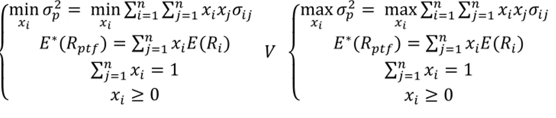
Alternatively, it is possible to follow a different resolution method suggested by Markowitz himself. It is in fact possible to set up a similar problem by developing two similar alternatives:

• Set up a system that maximizes the return value for a given variance level; • Set up a system that minimizes variance for a given performance

(26)

In both cases a further condition will then be imposed: the total use of the available resources (without resorting to indebtedness). The above can be summarized with the expression ∑6"=/𝑥" = 1.

Furthermore, we consider a context in which short sales cannot be carried out, that is, sell shares of which the property does not belong to us by hoping to buy them at a lower price in a second moment at the price agreed upon delivery to the buyer.

The above can be summarized by setting the following two systems:

⎩

⎪

⎨

⎪

⎧

min

{'

𝜎

U 4

_{= min}

{'

⎪

⎨

⎪

⎧

max

{'

𝜎

U 4

_{= max}

{'

∑

𝑥

"

𝑥

<

𝜎

"< 6 <=/ 6 "=/

𝐸

∗

_(𝑅

U$V

) = ∑

The above has a remarkable application in the geometric field: all the possible portfolios obtainable through a rational choice of yield and variance generate an area. This section is delimited by a set of combinations that constitute the efficient frontier. All the points belonging to this border represent the dominant portfolios.

Defined as an iso-mean line the set of all the points obtained by varying the weights of the single titles and keeping constant the yield and iso-variance curves the set of points obtained by varying

(27)

the weights of the single titles and keeping constant the variance, it is possible to identify a critical line at their points of tangency. Moving along the critical line it is possible to identify the lower limit of the portfolios selectable by the investor.

At this point it is necessary to understand how to build an efficient frontier and select the combination of portfolio that optimizes the choices of the investor. To simplify the presentation, a portfolio case consisting of only 2 securities will be presented first to then extend the reasoning to a generic valid case for portfolios consisting of n securities.

2.5 Construction of the Frontier Efficient in the case of 2 titles

Suppose you have a stock portfolio consisting of only 2 securities and invest all the available resources in it 𝑥l= (1 − 𝑥j). Knowing the performance of the two titles allows you to calculate

the yield of the given portfolio by setting an equation that contains only one unknown:

𝑅_U$V = 𝑥_j𝑅_j+ (1 − 𝑥_j)𝑅_l (2.12) Since it has been established that the total weight of the securities is equal to one and the formula just presented represents a convex function, it can be stated that the value obtained relating to the portfolio risk is between the risk of the A security and the risk of the title B.

This is also applicable to the expected value and variance of the portfolio:

𝐸X𝑅_U$VY = 𝑥_j𝐸(𝑅_j) + (1 − 𝑥_j)𝐸(𝑅_l) (2.13) 𝜎_U$V4 _{= 𝑥}

j4𝜎j4+ (1 − 𝑥j)4𝜎l4+ 2𝑥j(1 − 𝑥j)𝜎jl (2.14)

Therefore, the standard deviation will result: 𝜎_U$V= €𝑥_j4_𝜎

j4+ (1 − 𝑥j)4𝜎l4+ 2𝑥j(1 − 𝑥j)𝜎jl (2.15)

However, as explained in paragraph 2.2, the standard deviation gives an idea of the riskiness of a portfolio but does not take into account the relationship with which the securities which make it up interact with each other. This information is the key to a diversification operation. Therefore, also in this case, it is appropriate to refer to the correlation coefficient (formula 2.5).

Taking the formula (2.6) and isolating the covariance 𝜎jl, it is possible to include 𝜌"< within the

formula 2.15. Therefore, the following formula will be obtained for 𝜎U$V:

𝜎_U$V= €𝑥_j4_𝜎

j4+ (1 − 𝑥j)4𝜎l4+ 2𝑥j(1 − 𝑥j)𝜌jl𝜎jl (2.16)

Resuming what has already been described in the previous paragraph, the correlation coefficient can take values that are limited to the range [-1; 1]. In order to fully understand how the correlation

(28)

coefficient affects the construction of an efficient frontier, it is necessary to expose three distinct cases in which 𝜌"< will assume different values:

• 𝜌_"<= 1

In this context, the two stocks are perfectly correlated (positively) and it is not possible to further diversify its share portfolio. Replacing the given value within the formula (2.16) you will get the following expression:

𝜎

_U$V

= €𝑥

_j4

_𝜎

j4

+ (

1 − 𝑥𝐴

)

2

𝜎

l4

+ 2𝑥

j

(1 − 𝑥

j

)𝜎

jl

(2.17)

As it can be easily guessed, having failed 𝜌"<, this expression represents a simple square root of the

square of a binomial. Therefore, it is simplified as follows:

𝜎U$V = €(𝑥j𝜎j+ (1 − 𝑥j)𝜎l)4= 𝑥j𝜎j+ (1 − 𝑥j)𝜎l (2.18)

In geometric terms, to derive a representation of what has been said it is necessary to find the relationship between standard deviation and expected return. To do this the formula (2.13) is taken up again and the common variable 𝑥j:

𝐸X𝑅U$VY = 𝑥j𝐸(𝑅j) + 𝐸(𝑅l) − 𝑥j𝐸(𝑅l) = 𝑥j𝐸(𝑅j) + (1 − 𝑥j)𝐸(𝑅j) (2.19)

So:

𝑥_j(𝐸(𝑅_j) − 𝐸(𝑅_l)) = 𝐸X𝑅_U$VY − 𝐸(𝑅_l)

𝑥

_j

=

‚Xƒ„(…Y)‚(ƒ†)

𝐸X𝑅

U$V

Y − 𝐸(𝑅

l

)

𝐸

(𝑅

_j

) − 𝐸(𝑅

_l

)

𝜎

j+

‰

1 −

𝐸X𝑅

U$V

Y − 𝐸(𝑅

l

)

𝐸

(𝑅

_j

) − 𝐸(𝑅

_l

)

Š 𝜎

l=

=

‚Xƒ„(…Y)‚(ƒ†) 𝐸(ƒ‡))‚(ƒ†)

(𝜎

j−

𝜎

l

)

+

𝜎

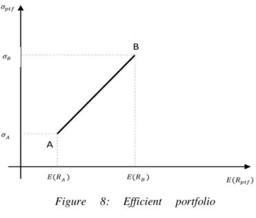
l (2.21)

(29)

As we can see from the formula (2.21), an increase in the expected return of the portfolio causes an increase in the standard deviation and, consequently, an increase in the risk. Moreover, as evidenced by the second representation of this formula, the standard deviation can be expressed as a convex combination of the standard deviations of the titles that compose it. In facts, the weight of the standard deviation of the title B is described as the difference between the total weight and the portion associated to the title A.

Tracing the graph using the expressions just obtained gives the following result:

The segment 𝐴𝐵 obtained represents the set of all efficient portfolio combinations. Therefore, it is not possible to identify a combination that guarantees a better performance without further increasing the risk.

• 𝜌"<= −1

This means that the positive change in the yield of a security causes a negative change to the return of the second security. In this context we have the maximum effect of diversification.

Proceeding as already illustrated for the first case, the value -1 of the correlation is replaced in the formula (2.16), obtaining the following result:

𝜎_U$V = C𝑥_j4_𝜎

j4+ (1 − 𝑥j)4𝜎l4− 2𝑥j(1 − 𝑥j)𝜎jl =

𝜎_U$V = €(𝑥_j𝜎_j− (1 − 𝑥_j)𝜎_l)4_{= |(𝑥}

j𝜎j− (1 − 𝑥j)𝜎l| (2.22)

Since the variables can take both a positive and a negative value, it is necessary to consider the result as an absolute value.

Figure 8: Efficient portfolio combination

(30)

At this point two distinct results can be obtained: • If 𝑥j𝜎j− (1 − 𝑥j)𝜎l > 0, then if 𝑥j>_\_‡\_,\†_†

Then the formula (2.22) will result as follows:

𝜎_U$V = 𝑥_j𝜎_j− (1 − 𝑥_j)𝜎_l = 𝑥_j(𝜎_j+ 𝜎_l) − 𝜎_l (2.23) • If 𝑥j𝜎j− (1 − 𝑥j) < 0, then if: 𝑥j<_\\†

‡,\†

Then the formula (2.22) will result as follows:

𝜎_U$V = 𝜎_l− 𝑥_j𝜎_j− 𝑥_j𝜎_l = 𝜎_l− 𝑥_j(𝜎_j+ 𝜎_l) (2.24)

To represent geometrically what has been said we rewrite the formulas (2.23) and (2.24) including within them the expected value of the return using the formula (2.20):

𝜎_U$V =‚Xƒ„(…Y)‚(ƒ†)

‚(ƒ‡))‚(ƒ†) (𝜎j− 𝜎l) − 𝜎l (2.25)

𝜎_U$V= 𝜎_l−‚Xƒ„(…Y)‚(ƒ†)

‚(ƒ‡))‚(ƒ†) (𝜎j− 𝜎l) (2.26)

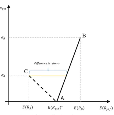
At this point it is possible to trace a representation:

Segment 𝐴𝐵 represents the set of efficient portfolios that can be obtained by varying the weights of the two securities. Segment 𝐴𝐶 represents instead the set of inefficient portfolios since, as can be seen from the chart, at equal risk it is possible to obtain higher returns.

(31)

It is possible to see that the condition of perfect negative correlation turns out to be a case that is difficult to find in real life. In fact, the equity portfolio created at point A would imply the possibility of investing in a combination that guarantees a relevant return at the expense of a zero risk.

In order to identify which is the combination that allows to obtain a portfolio at zero risk, the standard deviation is set equal to 0. Starting from the formula (2.22), we will have:

|𝑥j𝜎j− (1 − 𝑥j)𝜎l| = 0

𝑥_j𝜎_j− (1 − 𝑥_j)𝜎l = 0

𝑥_j𝜎_j+ 𝑥_j𝜎_l− 𝜎_l = 0 𝑥_j(𝜎_j+ 𝜎_l) = 𝜎_l Therefore, the proportion will be calculable as:

𝑥_j= \†

(\‡,\†) and (1 − 𝑥j) =

\‡

(\‡,\†)

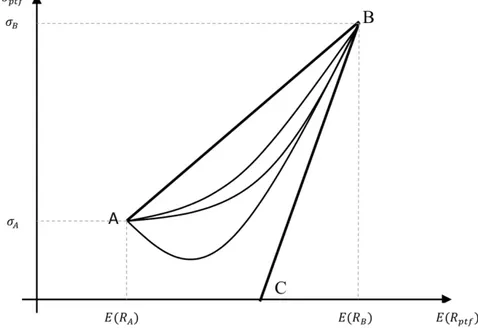
• −1 < 𝜌_"<< 1

The peculiarity of this context is that, contrary to the cases of perfect correlation (positive or negative), the expected variance-value relationship does not generate a linear function, but a curvilinear one. This phenomenon is due to the fact that as the value of the correlation coefficient decreases, the possibility of diversification increases:

(32)

As the correlation coefficient decreases, the curvilinear moves from the segment 𝐴𝐵 to the segment 𝐵𝐶. The area delimited by points A, B and C represents the set of all the combinations that can be obtained using the securities comprising the equity portfolio.

2.6 Construction of the Frontier Efficient in the case of n> 2 titles

Usually an equity portfolio consists of a large number of securities. Without prejudice to the hypotheses of identification of efficient combinations discussed in paragraph 2.3, it is necessary to take into account a further factor: the relationship between the securities. An effective method to solve this problem is provided by the variance-covariance matrix, i.e. a matrix that has the following characteristics:

• It is a matrix having the same number of rows and columns (Square Matrix) • Its main diagonal is the variance of the securities that make up the portfolio. The variance-covariance matrix (S) can be calculated with the following formula:

𝑆 =

j•{ j

‘

(2.27) Where is it:

• 𝐴 represents the matrix of refuse of the returns from the average; • 𝐴’_{represents the transposed matrix of A;}

• M represents the number of returns considered.

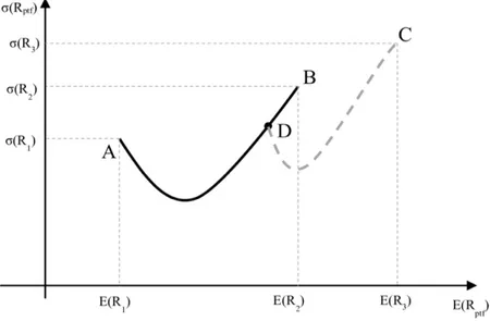
As analysed in the previous paragraph, it is possible to graphically represent the realization of an efficient frontier by relating standard deviation and expected value. Contrary to what was observed in the case of a portfolio consisting of only 2 securities, in the case of a larger number of securities it is not possible to obtain a limited area that includes the possible portfolio combinations.

Assuming you have an equity portfolio consisting of three securities (A, B, C) and known their expected return and their standard deviation, it is possible to obtain the following representation:

(33)

Apparently, the curve defined by the ADC section would seem to represent the set of efficient portfolios, however it is not so since the combinations offered by point B are not taken into account. Therefore, the most appropriate construction is that dictated by the AEC section. All the points contained in this curve outline the set of possible portfolios, while below this sector all the impossible combinations of the titles are placed. Recalling the characteristics of the previously dominant principle of dominance, it can be stated that the efficient frontier is given by the portion of the curve defined by points E and C. Point E also represents the combination of the securities that make up the portfolio with minimum variance.

In order to obtain a portfolio consisting of three securities, it is possible to distinguish the transaction in two distinct phases. The first of these involves obtaining an equity portfolio consisting of only two securities, retracing the steps illustrated in the previous paragraph. The second phase consists of a convex combination from the newly obtained portfolio and the third title taken into consideration.

Assuming to be in a context where the correlation is −1 < 𝜌"< < 1. We can indicate with A and B

two titles with standard deviation 𝜎/ and 𝜎4 of expected value of the return equal to 𝐸(𝑅/), 𝐸(𝑅4).

Remembering that the sum of the weights of the two titles is equal to 1, it is possible to obtain the efficient frontier represented by the following graph:

Point D represented in the figure represents one of the possible border portfolios. It will have a standard deviation of 𝜎U$V and expected return equal to 𝐸X𝑅U$VY.

(34)

Now it is possible to include a third C title with standard deviation equal to 𝜎“ and expected return

equal to 𝐸(𝑅”). The introduction of this title in the equity portfolio must guarantee in any case that

the total weight of the securities is equal to 1:

Along the curve obtained through points D and C, it is possible to identify all the possible portfolio combinations obtainable by including the title C within the portfolio previously obtained through a convex combination of securities A and B. By indicating with z a generic portfolio obtainable from the border 𝐷𝐶, it is possible to obtain the standard deviation using formula (2.17):

Figure 12: Expected value of returns

(35)

𝜎_• = C𝑥_/4_𝜎

U$V4 + (1 − 𝑥/)4𝜎”4− 2𝑥/(1 − 𝑥/)𝜎U$V,“

𝜎U$V,“ represents the only unknown of the equation presented. However, it is possible to derive it by

analysing the relationship between the returns of the portfolio consisting of two securities and the title C.

Point D represents only one of the possible portfolios obtainable through a combination of securities A and B. Therefore, if one wants to identify every possible portfolio obtainable from the combination of the three titles, it is necessary to take into consideration every single point belonging to the frontier constituted by the titles A and B.

The area obtained in figure 14 represents all the possible portfolio combinations obtainable using the three titles A, B and C.

As can be seen from the graph, the function obtainable from the combination of the three titles is growing and convex. This implies that an increase in the expected value of the return is accompanied by a more than proportional increase in the standard deviation and, therefore, in the risk.

2.7 Selection of the optimal portfolio

Once the procedure of creation of the efficient frontier has been clarified, it is necessary to make a final statement. The methods analysed in the previous paragraphs allow the investor to have a picture of all the possible combinations that maximize his investment. However, they do not allow to select

(36)

the combination that takes into account the preferences of the individual and therefore allows to obtain the risk-return ratio most suitable for its characteristics. To take this into account it is therefore necessary to resort to a subjective variable that captures these elements: the indifference curve. The indifference curve is the Cartesian representation of the investment choices that provide the individual with the same utility and which therefore make him indifferent to the alternatives obtained. Using a map of all the indifference curves, i.e. a set of curves that summarize for each utility level a set of indifferent choices, it is possible to derive a utility function expected using the expected return as variable. Specifically, the work proposed by H. Markowitz uses an expected squared utility function, which is a function that summarizes the preferences of the individual using two variables (risk and expected portfolio return) and which takes into account his risk aversion. This last yield gives the indifference curves a concave nature since, to compensate for an increase in risk, the individual requires a certain increase in yield.

The expected utility function can be represented as follows:

𝐸(𝑈(𝑥)) = 𝐸X𝑅

_U$V

Y −

/₄

𝜆𝜎

_U$V4

_(2.28)

Where 𝜆 summarizes the degree of risk aversion of the individual.

Graphically it is possible to represent the expected utility function by reporting the mapping of the indifference curves and the efficient boundary (𝐹𝐸𝑝𝑡𝑓) obtained as described in the previous paragraphs:

The point U, obtained as a point of tangency between the efficient boundary and the indifference curve, represents the optimal choice of the investor. This combination takes into account both objective factors (obtaining efficient combinations using the dominance principle) and subjective

(37)

factors (recourse to indifference curves to select the portfolio most suited to the characteristics of the individual).

To apply the procedure presented above it is necessary to assign a numerical value to the degree of risk aversion 𝜆. It is therefore necessary for the investor to be able to translate his preferences into analytical terms. Although this is not always easy to implement, the method provided by the expected utility function is certainly the most used in modern finance.

2.8 Limitations of Portfolio Theory

The portfolio allocation theory proposed by H. Markowitz represents the first step of approach to the study of finance. However, there are several limits that make the proposed theory difficult to apply in a real context.

In order to identify the efficient combinations of the securities, only two variables are taken into account (expected return and standard deviation) precluding other possible references. Furthermore, the use of the standard deviation as a risk estimation tool limits the actual forecast of the loss by analyzing only the variations in returns and does not provide a picture of the maximum possible loss.

During the selection phase of a portfolio, only risky securities are considered, making the diversification operation ineffective, since all other investment activities are neglected. Furthermore, a change in the estimate of one of the two parameters (expected return and standard deviation) can cause a noticeable change in the distribution of the securities that make up the share portfolio. Starting from these factors, various theories have been developed which, although maintaining the starting hypotheses, try to remedy the limits highlighted in the work of H. Markowitz. Some of them will be proposed in the next paragraph.

2.9 Overcoming the limits of Portfolio Theory: the CAPM

As anticipated in paragraph 2.7, the Portfolio Theory proposed by H. Markowitz, although it is of considerable relevance and of great impact during the market analysis, has relevant limits. In order to overcome these limitations, a considerable number of research and studies have been conducted. Among these, the theories presented by three economists stand out for their importance and effectiveness: W. Sharpe, J. Lintner and J. Mossin.

(38)

W. Sharpe (“A Theory of Market Equilibrium under Conditions of Risk”, The Journal of Finance) collaborated with Markowitz's studies, sharing the 1990 Nobel Prize with him and with M. Miller. He formulated two hypotheses13 additional to those already proposed by the mentor of his theory. It states that all investors have the same expectations on the expected returns and risks of a security and that there is always a security with a certain return and no negotiable risk without being subject to limits.

J.Mossin worked on the stud of W.Sharpe assuming a context in which the uniperiod context proposed by Markowitz was applicable to all investors and that the market was perfect and able to incorporate all the information relating to its financial instruments.

The first step is to include a risk-free security in the equity portfolio. For simplicity of calculation a BOT is used (ordinary Treasury voucher) since it is a title without coupons and has an annual frequency. Having a short duration and being guaranteed by the State (therefore risk-free), it is reasonable to expect a very low return.

It is assumed that a portfolio consisting of only 2 securities is available, one risk-free (BOT) and one risky.

Recalling the formulas (2.13) and (2.15), it is possible to calculate the expected return and the standard deviation of the considered portfolio, remembering that the BOT has zero standard deviation since it is free of risks (consequently also the covariance will be equal to 0):

𝐸(𝑅_U™V) = 𝑥_j𝐸(𝑅_j) + (1 − 𝑥_j)𝐸(𝑅_V) (2.29) σ_U$V = C𝑥_j4_σ

›

4 _{+ (1 − 𝑥}

j)4σ›4+ 2𝑥j(1 − 𝑥j)σ›œ= C𝑥j4σ›4 = 𝑥jσ› (2.30)

Following the same path presented in paragraph 2.3, the relationship between expected return and standard deviation is highlighted. By including the formula (2.20) inside the (2.30) the following result is obtained:

𝜎

_•žœ

=

\‡

‚(ƒ‡))ƒ…

𝐸X𝑅

U$V

Y −

\‡

‚(ƒ‡))ƒ…

𝑅

V

(2.31)

In geometric terms, this function is represented by a semi-straight line:

As can be seen, in this representation 𝑥j can also assume values greater than 1 since it was

(39)

The relationship between standard deviation and expected return represents the angular coefficient of the represented line. Therefore, it will assume the value _‚(ƒ\‡

‡))ƒ…

Of great importance is the reciprocal of the expression just obtained:

𝜃 =

‚(ƒ‡))ƒ…

\_‡ (2.32) 𝜃 represents the Sharpe Index, i.e. the extra return obtainable from a risky security (with respect to a certain return) related to its risk.

Taking the formula (2.31) it is possible to express the expected return of the portfolio based on the standard deviation:

𝐸X𝑅_U$VY = 𝑅_V+‚(ƒ‡))ƒ…

\‡ 𝜎U$V (2.33)

From this point, it is possible to state that the expected return can be defined as a combination of the yield of the risk-free security and a portfolio consisting of risk assets.

At this point it is necessary to identify which combinations make the portfolio analysed effective. However, it is not possible to proceed as illustrated by H.Markowitz since in this context the securities are not considered risk-free.

Bancassurance : from organization to the wealth management and Armundia case

POLITECNICO DI MILANO

School of Industrial and Information Engineering

Master of Science in Management Engineering

Bancassurance: from the organization to the wealth

management and Armundia case

Relator: Prof. Laura Grassi

Correlator: Prof. Davide Lanfranchi

Author:

Mattia Dario Andreoli (878239)

Table of contents

Index of figures

Index of Tables

Sommario

Abstract

Chapter 1: MiFID and IDD, the customer as new focal point

1.1 MiFID II

Customer Protection

Reporting

requirements:

Transparency

Scope of trading

requirements

changed to

include:

Market Infrastructure

1.2 IDD

1.3 Points of contact and Italian view

Chapter 2: how to create a financial portfolio according to new

directives

2.1 Markovitz and the theory of portfolio selection

2.2 Performance and variance analysis

𝑟

=

𝐸(𝑅

) = ∑

𝑟

𝑝

2.3 Composition of a Share Portfolio

𝜌

=

𝐸W[𝑅

− 𝐸(𝑅

)]^𝑅

− 𝐸X𝑅

Y_Z =

= ∑

∑

𝑥

𝑥

𝜎

2.4 Optimize a Portfolio: Principle of Dominance

⎩

⎪

⎨

⎪

⎧

min

𝜎

= min

∑

∑

𝑥

𝑥

𝜎

𝐸

(𝑅

) = ∑

𝑥

𝐸(𝑅

)

∑

𝑥

= 1

𝑥

≥ 0

𝑉

⎩

⎪

⎨

_{= min}

_(𝑅

_{= max}

_(𝑅

_𝜎