An investigation of piano transcription algorithm for jazz music

(1)

POLITECNICO DI MILANO

Master’s Degree in Computer Engineering Department of Electronics and Information

Technology

AN INVESTIGATION OF PIANO

TRANSCRIPTION ALGORITHM

FOR JAZZ MUSIC

Supervisor: Prof. Fabio Antonacci, Politecnico di

Milano

Co-supervisor: Prof. Peter Knees, Technische

Universit¨

at Wien

Co-supervisor: Richard Vogl, Technische Universit¨

at

Wien

Master Thesis of:

Giorgio Marzorati, ID 876546

(2)

“ Never say never.

Because limits, like fears are often just an illusion.”

(3)

Abstract

The thesis aims to create an annotated musical dataset and to propose an Automatic Music Transcription system specific to jazz music only. Although many available annotated datasets are built from the audio recordings, the proposed one is built from MIDI file format data, providing robust annota-tion. The automatic polyphonic transcription method uses a Convolutional Neural Network for the prediction of the outcome.

Automatic Music Transcription is an interesting and active research field of Music Information Retrieval. Automatic Music Transcription refers to the analysis of the musical signal to extract a parametric representation of it, e.g. a musical score or MIDI format file. Even for man, the transcription of music is difficult and still remains a hard task requiring a deep knowledge of music and high level of musical training. Providing a parametric representation of audio signals would be important for application to annotated music for automatic research in large and interactive musical systems. Massive sup-port would be given to the musicology fields producing annotation for audio performance without any written representation, and to the education field. The work hereby presented is focused on the jazz genre, due to its variety of styles and improvisation parts, of which usually there is no available tran-scription, and to which the field of Automatic Music Transcription can be of help. Its variability makes the problem of Automatic Music Transcription even more challenging and also for that reason there is not much work avail-able.

Results of the transcription system highlighted the difficulties of transcribing jazz music, compared to classical music, but still comparable to state-of-art methodologies, producing an f-measure of 0.837 testing the Neural Network on 30 tracks of MAPS dataset and 0.50 from the jazz dataset experiment.

(4)

Acknowledgment

I would first like to thank my thesis advisor Professor Fabio Antonacci of the Computer Engineering Department at Politecnico di Milano, whose exper-tise, diligence and patience were crucial in writing this thesis. He consistently allowed this dissertation to be my own work, but steered me in the right di-rection whenever he thought I needed it.

I would also like to thank the experts who were involved throughout the entire developing phase of this research project: my foreign advisor in Vi-enna, Professor Peter Knees and assistent Richard Vogl of the Informatic faculty of Technische Universit¨at Wien. Without their passionate participa-tion and input, it could not have been successfully conducted.

I must express my very profound gratitude to my parents and to my fam-ily for providing me with unfailing support and continuous encouragement throughout my years of study and through the process of researching and writing this thesis.

Finally, I would like to thank all my true friends for showing me constant love and support. This accomplishment would not have been possible with-out them. Thank you.

(5)

List of Figures

3.1 Fletcher Munson diagram . . . 20

3.2 MIDI network scheme . . . 23

3.3 Voice channel assignment of the four modes that are supported by the MIDI: top left Omni on/poly; top right Omni on/mono; bottom left Omni off/poly; bottom right Omni off/mono . . . 26

3.4 Convolutional Neural Network scheme . . . 31

3.5 Deep Neural Network scheme. Left: Forward Neural Network; Right: Recurrent Neural Network . . . 31

3.6 Long Short-term cell . . . 32

4.1 System workflow . . . 34

4.2 Convolutional Neural Network list of layers used in the thesis . 41 4.3 Electric Piano Fender Spectrogram . . . 43

4.4 Hammond B3 Spectrogram . . . 44

4.5 Electric Grand U20 Spectrogram . . . 44

4.6 Crazy Organ Spectrogram . . . 45

4.7 Electric Grand Piano Spectrogram . . . 46

4.8 Fazioli Grand Bright Piano Spectrogram . . . 46

5.1 FF-mpeg operational scheme . . . 55

5.2 Database scheme . . . 62

6.1 Sensitivity and Specificity metrics . . . 66

6.2 Diatonic A major scale. Top: Predictions; Middle: Target; Bottom: Spectrogram . . . 69

6.3 Diatonic C major scale. Top: Spectrogram; Middle: Target; Bottom: Predictions . . . 70

6.4 Simple jazz performance. Top: Spectrogram; Middle: Target; Bottom: Predictions . . . 70

(8)

6.5 Articulated jazz performance. Top: Spectrogram; Middle: Target; Bottom: Predictions . . . 71 6.6 Jazz performance affected by octave errors. Top:

(9)

List of Tables

2.1 Multiple-F0 estimation approaches organized according to

time-frequency representation employed . . . 11

2.2 Multiple-F0 techniques organized according to the employed technique . . . 11

4.1 Evaluation metrics for SoundFonts tested on a C-major scale . 43 4.2 Evaluation metrics tested with different window size . . . 45

5.1 Distribution of piano program . . . 58

5.2 Madmom results for the three splits . . . 63

6.1 Evaluation metrics for MAPS dataset . . . 68

6.2 Evaluation metrics for Jazz dataset . . . 68

6.3 Accuracy measure . . . 72

(10)

Chapter 1 Introduction

1.1 The challenge of Automatic Music

Tran-scription

Automatic Music Transcription is the process that allows the extraction of a parametric representation of a musical signal through its analysis. Researches has been undertaken in this field of study for 35 years starting with Moorer [1], and cover specific areas of monophonic and polyphonic music. Auto-matic transcription for monophonic streams is widely considered a problem already solved [2]; as a matter of fact, transcriptions with the highest rates of accuracy are actually obtainable for any musical instrument. Polyphony, on the contrary, has manifold intrinsic complexities to be considered that constrain the research to specific cases of study and analysis for a possible automatic transcription. The difficulties to achieve reasonable results thus indicate that improvements and streamlined approaches are necessary to the Automatic Music Transcription of polyphonic music signals, underlining in it the true challenge of this subject.

Automatic Music Transcription is a complex system divided into subtasks: pitch estimation, related to the detection of a given time frame, onset and offset detection of the relative pitch, loudness estimation, and finally instru-ment recognition and extraction of rhythmic pattern. The core task of AMT applied to polyphonic music, is the estimation of concurrent pitches, also known as multiple-F0 or multi-pitch estimation. Depending on the number of subtasks, the output of an AMT system can be a simple representation, such as MIDI or piano-roll, or a complex one, such as an orchestral score.

(11)

An AMT system has to solve a set of MIR problems to produce a complete music notation, central to which is the multi-pitch estimation.

Other features should be included in the representation in order to improve the transcription performance, such as descriptors of rhythm, melody, har-mony and instrumentation. The estimation of most of these features has been studied as isolated tasks, as instrument recognition, detection of onset and offset, extraction of rhythmic information (tempo, beat, musical timing), pitch estimation and harmony (key, chords). Usually, separated algorithms are required for each individual result. Considering the complexity of each task this is necessary, but the main drawback is the combination of outputs from different systems or the creation of an algorithm to perform the joint estimation of all required parameters.

Another challenge is represented by the non-availability of data for evaluation and training. This is not due to a shortage of transcriptions and scores, but to the human effort required to digitize and time-align the music notation to the recording. The only exception is represented by the piano solos thanks to the available data from the MAPS database [3] and the Disklavier piano dataset.

1.2 Scope of the thesis

The thesis has a double aim: to create an annotated musical dataset com-pletely dedicated to jazz music and to propose a specific AMT system specific to polyphonic jazz recordings. The AMT method is based on the estimation of multiple-pitch and onset detection using a Neural Network algorithm. Annotated music plays a central role in Multi-Pitch estimation and Auto-matic Music Transcription. A great amount of data is required for the de-velopment and evaluation of such algorithms which rely on statistical ap-proaches. However, such data is usually embedded in annotated sound databases, some of which are public, while others, as those used in the MIREX context, are private. Few databases are currently available and usu-ally consist of musical instruments and recordings from which the annotated file is derived with the ensuing problem of inaccurate and erroneous values for pitch, onset and offset time.

The choice of working with jazz genre for the AMT system was mainly justi-fied by the lack of specific works, and hence the need of gathering a dedicated dataset. On the other hand, the choice is also motivated by the genre itself,

(12)

as jazz comprises a wide variety of different styles and ways of performing the same musical pieces. Jazz is a genre that is renowed for its syncopated rhythms and chord progression, the improvisational phrasing, the intimate expressiveness and the articulated melodies. It is best defined in the words of one of the greatest trumpeters Wynton Marsalis: ”Jazz is not just, ”Well, man, this is what I feel like playing .” It is a very structured thing that comes down from a tradition and requires a lot of thought and study.”.

Usually, opening and closing parts of jazz compositions are characterized by a melody or theme and the specified progression of chords, while the central part is often covered by the solos in a cyclical rhythmic form [4]. Impro-visation is a process of elaboration of a melodic line, specified in the lead sheet or score [4]. During this action, the music sheet is a constant refer-ence for the rhythm and the harmony, but the melody is subject to a live reinterpretation. Furthermore, the improvisation is the moment in which the performer may show its virtuosism and its personal style, that is expressed by the use of special musical effects, such as vibrato or slide, or dynamic emphasis. This very peculiar characteristic influenced Jazz music itself; so for the same composition it is possible to find recordings of the same artist quite different among them (like two performances of Blue Train by John Coltrane [5] [6]).

For this reason, one of the advantages of employing AMT to Jazz could be the relevant consequence for musicological studies of specific artists, for deep-ening their styles and performances.

Furthermore, due to its spontaneous and creative origin, improvisation ap-pears not to follow any harmonic rule or pattern and for this reason could be a good benchmark for transcription [4].

Finally, the choice of focusing the research on the piano only has technical and conceptual reasons. In part, due to the diffused knowledge of the instrument and the large available datasets of synthesized and annotated recordings; in part, because of its double role in jazz music: the lead voice (performing the melodic part and the improvisations), and the accompaniment.

(13)

1.3 Aims and applications

Automatic Music Transcription converts audio recording into its paramet-ric representation using a specific musical notation. Despite progress in the field AMT research, no end-user applications with accurate and reliable re-sults are available and even the most recent AMT products are clearly infe-rior compared with human performance [7]. Although the Automatic Music Transcription of polyphonic music cannot be considered a solved problem, it is of great interest due to its numerous applications in the field of music technology.

Music notation is an abstraction of parameters. It is a precise organization of symbols just like words or letters are for languages and the Western mu-sic notation is still considered the most important and efficient medium of transmission of the music. Human music transcription is a complicated rou-tine that requires high competence in the musical field and musical training, and it is also a time-consuming process [2]. A its most basic, AMT allows musicians to convert live performances into music sheets and thus easily tran-script their performances [8] [9]. For this reason AMT is of special interest for musical styles when no score is available, e.g. folk music, jazz and pop [10] or for musicians that are untrained towards the western notation. Another field in which AMT would be extremely useful is the analysis of non-written musical pieces, musicological one and musical education [9] [11] [12]. It would allow the investigation of improvised and folk music, simply by retrieving information on the melody. This last application is of particu-lar interest for jazz case study, due to the wide use of improvisation during live performances. A clear example is represented by the two performances of Blue Train by John Coltrane, very different from each other despite the same lead sheet: the first is the live concert in Stockholm in 1961 [5], the second is the mastered piece [6]. It would allow us to focus on the detection of personal fingerprint of an artist.

Musical notation does not only allow the reproduction of a musical piece, but it also allows modification, arrangement and processing of music at a high level of abstraction. Another interesting application of music transcrip-tion, that has emerged in the last few years, is structured audio coding [10]. Structured audio representation is a semantic and symbolic description of ultralow-bit-rate transmission and flexible synthesis that uses high-level or algorithmic models, such as MIDI [13].

(14)

More recently it has been applied to the automatic search and annotation of new musical information, or to interactive musical systems, such as com-puters actively participating in live performances, score following or rhythm tracking. In fact, this kind of support of live performances would be very helpful for the musicians, who could freely express themselves without both-ering about the musical annotations from where their musical inspiration flow. On the other hand, musicians usually see automatically created com-positions and accompaniment as not achieving the same level of the quality. The query by humming MIR task is one of the most recent applications of the AMT to the slof´ege of a melody, where the output of an AMT can be used as a query for an interactive musical database.

1.4 Structure of the thesis

Chapter 2 presents an overview of the main Music Information Retrieval tasks and methodologies applied to the jazz genre. It begins with the description of what MIR and Automatic Music Transcription are. Then it goes on to explain in depth how transcription can be broken down into MIR tasks. The third chapter is dedicated to the general concepts and terminology useful for the understanding of the following chapters. It gives a brief overview of the main application considered in the thesis, as well as musical sound formal description, deep learning, MIDI and Music Information Retrieval. Finally, it describes different approaches in which to deal with the problem of Auto-matic Music Transcription.

The subsequent sections represent the core of the thesis and explain the method applied, the proposed dataset and finally present results and consid-erations.

Chapter 4 is focused on the description of the approach used in the thesis, based on machine learning, and presents the complex workflow required for obtaining results, through the various system blocks. And finally it provides an in-depth explanation of the pre-processing and Neural Network stages. Section 5 is dedicated to the presentation of the dataset creation process, starting from the collection of raw MIDI files, passing through the analyti-cal phase, ending with the synthesis. The chapter also deals with the main design choices made during the building of the dataset and with the main software used.

(15)

The final two sections are dedicated to the explanation of the metrics to obtain the results, the evaluation to the presented system and ends with a summary of the main contributions to the thesis, offering a perspective on improving this system and the potential application of the transcription system.

(16)

Chapter 2 Related works

The following chapter gives an overview of Automatic Music Transcription problem. The first section is focused on the description of the transcription problem with historical references, to give an idea of the evolutive trend. The remaining sections are dedicated to the subtasks of state-of-the-art Au-tomatic Music Transcription presentation. A brief description of the single pitch estimation problem was inserted for the sake of completeness. De-spite not being the focus of the thesis, it should give a good explanation of the differences in the multi-pitch estimation. Finally multi-pitch estimation state-of-the-art is presented in depth to evaluate different algorithms and methodologies.

2.1 Overview on Automatic Music

Transcrip-tion

Automatic Music Transcription is thought to be the process to translate an audio signal into one of its possible parametric representations. As explained in section 1.3, there are many applications in this research area, in particular applied to musical technology and to musicology.

Automatic Music Transcription is deeply linked to Music Information Re-trieval. The latter is defined as a research field focusing on the extraction of features from a musical signal. These features need to be meaningful to the task of understanding musical content as the auditory human system does. The features extracted can be of different levels depending on the type of information contained.

(17)

Actually, Automatic Music Transcription can be decomposed into sub-tasks related to the mid-level features of MIR. Onset and offset detection, beats, downbeats and tempo estimation are some of them.

The main tasks for an AMT system are the pitch estimation and the onset de-tection. This chapter focuses on these problems and the different approaches used in the state-of-the-art methodologies.

2.2 Automatic Music Transcription history

First attempts of AMT systems being applied to polyphonic music date back to the seventies. They showed many limitations concerning polyphony level and a number of voices. Moorer [1] method was based on the autocorrela-tion of output from a comb-filter, delaying the same input signal to find a pattern in the signal. Blackboard systems came into the AMT scene at the end of the century. Martin [14] [15] proposed a method based on five levels of knowledge ranging from the lowest to highest ones: raw track, partials, notes, melodic intervals, and chords. Blackboard systems are hierarchically structured, and the integrated scheduler determines the order of the action to perform. Nowadays most of the technique can be related to Probability-based techniques, Spectrogram Factorization, Machine Learning, and Signal Processing ones.

A straightforward procedure is offered by the Signal Processing approaches like the Klapuri one [16]. Klapuri proposed in the starting year of 2000 a method where fundamental frequencies, once estimated from the spectrum of the musical signal, are removed from the signal iteratively.

During the same period, more complicated techniques were employed in order to tackle the probabilistic character of the signal. The Goto [17] approach introduced a method for detecting predominant fundamental frequencies tak-ing into consideration all possibilities for F0.

More recent works exploit spectrogram factorization techniques like Non-Negative Matrix Factorization.

As the maths could suggest, the magnitude spectrum of a short-term signal can be decomposed into a sum of basis spectra, representing the pitches. They can be fixed by training on annotated files, or estimated from observed spectra. NMF estimates the parameters of the model. The Vincent [18] method (2010) used harmonicity and spectral smoothness constraint for an NMF-based adaptive spectral decomposition.

(18)

The probabilistic variant of NMF is PLCA studied by Smaragdis [19] (2006) and Poliner [20] (2010).

Finally, machine learning techniques seem to be the most promising and generalizable methods, capable of achieving better performances in terms of reliability. The Support Vector Machine, a supervised machine learning al-gorithm, was used by Poliner and Ellis [21] (2006). They trained the SVM on spectral features to have a frame-based classification of note instances. HMM was used to introduce temporal constraint during the elaboration of detected note events. Sigtia et al. [22] (2014) exploited the RNN capabil-ity of capturing temporal structure in data and MLM to generate a prior probability for the occurrence in the sequence to improve the transcription.

2.3 Single-pitch estimation

Single pitch estimation refers to the detection of the pitch in monophonic tracks, where monophonic means that no more than one voice and pitch at a time can be present in each time frame. This massive initial hypothesis simplifies the task and the problem of single pitch estimation both for the speech and for the musical signals is taken as solved.

Chevign´e’s dissertation [23] takes an overview on various single-pitch meth-ods dividing them into framework using spectral components, temporal ones, and spectro-temporal ones.

Spectral methods use spectral components relying on the analysis of the frequency element within each note. Since musical sounds are considered quasi-harmonic signals, it can be stated that partials will be at integer mul-tiples of the fundamental frequency. The energy spectrum should have a maximum indicating the fundamental frequency. Different spectral meth-ods exploits different algorithm for the detection of pitch. Autocorrelation, cross-correlation and maximum likelihood functions are the most used de-pending on the representation employed. Spectral techniques are affected by harmonic errors placed at integer multiples of the fundamental one.

Temporal methods make use of autocorrelation function for the estimation of the fundamental frequency from raw audio signals. Due to the periodicity of audio signals, peaks in the function indicate the targets. Among them, fundamental frequency of the waveform would be the first peak, the other represents sub-harmonic errors due to higher harmonic components.

(19)

from their approaches. The signal is segmented in short frequency range as in Hewitt’s work [24]. The proposed model exploits the human auditory system making use of a log-spaced filter-bank in the first stage of the framework. An autocorrelation function will detect the pitch for each channel of the filter-bank. A summary autocorrelation to merge all the information from all the frequency bands is required for overall results.

2.4 Multi-pitch estimation

Polyphonic music is usually characterized by multiple voices or instruments and multiple concurrent notes in the same time-frame. This led to the im-possibility of making any assumption about the spectral content of a time frame. A couple of papers highlight a good division of multi-pitch estimation methods, as for single-pitch estimation, in temporal, spectral and spectro-temporal methods. The paper [23] suggests that most of the methods are based on the spectral features analysis. However, within the same set of representations, it also focuses on many differences concerning the used tech-nique. Furthermore, the paper from Benetos [25] explains in depth all the state-of-the-art methods separated by the employed techniques.

The pitch extraction method can be a way of classifying different multi-pitch estimation approaches. As a matter of fact, joint algorithms are computa-tionally heavier than iterative algorithms. Unlike the iterative ones, joint methods do not introduce errors at each iteration. In fact, iterative methods extract pitch at each iteration usually subtracting the estimated pitch till no more fundamental frequencies can be detected. These kinds of methods tend to accumulate errors but are really light computationally speaking. On the other hand, joint algorithms try to extract a set of pitches from the single time-frame. In table 2.1, some multi-pitch estimation methods are divided according to which kind of time-frequency representation is used.

(20)

Time-Frequency Representation Citation

Short-Time Fourier Transform Klapuri [16] Yeh [26] Davy [27] Duan [28] Smaragdis [19] Poliner [21]

Constant-Q Transform Chien [29]

Constant-Q Bispectral Analysis Argenti [27]

Multirate Filterbank Goto [12]

Resonator Time-Frequency Image Zhou [27]

Specmurt Saito [30]

Wavelet Transform Kameoka [31]

Adaptive Oscillator Networks Marlot [10]

Table 2.1: Multiple-F0 estimation approaches organized according to time-frequency representation employed

One of the most used representations is the Short-Time Fourier Transform, because of the easy fruition of a fast and robust algorithm and because of the deep technical knowledge of that method. However, the Short-Time Fourier Transform has the main problem of using a linear frequency scale. To overcome this issue other representations can be used like Q-transform, which employs a logarithmic frequency scale using constant ratio between harmonic components of a sound, or other kind of filter-banks. Finally, the specmurt is a representation of the signal based on the inverse Fourier Trans-form of a spectrum calculated on log-frequency.

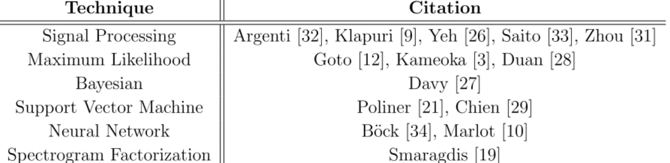
Technique Citation

Signal Processing Argenti [32], Klapuri [9], Yeh [26], Saito [33], Zhou [31] Maximum Likelihood Goto [12], Kameoka [3], Duan [28]

Bayesian Davy [27]

Support Vector Machine Poliner [21], Chien [29]

Neural Network B¨ock [34], Marlot [10]

Spectrogram Factorization Smaragdis [19]

(21)

Table 2.2 was built following the division concerning the used technique for the multi-pitch extraction. In particular, it shows the majority of meth-ods exploits signal processing techniques. In this case, extracted audio fea-tures are used in the multi-pitch estimation without the help of any learning algorithm. Methods based on the spectrogram factorization, such as Non-Negative Factorization Matrix, are more recent. Those kind of algorithms try to analyze the input space in order to decompose the signal representation in time-frequency. Other methods rely on probability concerning signal field, exploiting Bayes formulation of a problem and using Monte Carlo Markov Chain in order to reduce computational costs and Hidden Markov Model as a post-processing system for note tracking.

Finally, learning algorithms are now increasingly used and seem to be the more promising methods. Supervised learning procedures such as Support Vector Machine for the multiple-pitch classification can also be found. For what concerns the unsupervised learning algorithm Gaussian Mixture Model and any Artificial Neural Network can easily be found in the literature. The following sections will go through each multi-pitch estimation technique highlighting the merits and defects of each one.

2.4.1 Signal processing techniques

Signal processing techniques are probably the most widespread for the de-tection of pitches within a single time-frame. The input signal is processed for the extraction of the representation which can be in the temporal or in the frequency domain. The detection of pitches is computed using a pitch salience function, also called pitch strength function, or a set of possible pitches.

Klapuri [16] exploited the smoothness of a waveform computing Magnitude Power Spectrum and filtering it with a moving average filter for the noise suppression. The Klapuri method is based on spectral subtraction with the inference of polyphony. A pitch salience function applied within a specific band, estimating the pitch from the spectrum. It also calculates the spec-trum to subtract it from the input signal in order to exclude the detected pitch from the input signal. Yeh [26] developed a joint multi-pitch estima-tion algorithm basing the detecestima-tion of the fundamental frequencies on a set of candidate pitches. The used spectro-temporal representation is the Short-Time Fourier Transform. A pre-processing stage is employed to estimate the

(22)

noise level present in the signal in an adaptive fashion. The pitch candidate score function takes into account different parameters like harmonicity fea-tures, mean bandwidth of the signal, spectral centroid, and synchrony. With reference to iterative methods, some were developed like the Zhou [27]. Zhou used a filter-bank composed of complex resonators that should approximate pitch representation. The energy spectrum is used as a representation of the audio signal. Rules for the iterative elimination of candidates pitches are based on the number of harmonic components detected in each pitch and a measure of spectral irregularity. Another mid-level representation used is the specmurt. It consists of the inverse Fourier Transform of the power spectrum computed in a logarithmic fashion. Saito [35] proposed a method based on it where the input spectrum can be seen as the convolution of harmonic struc-tures and pitch indicator functions. On the other hand, the deconvolution of the spectrum by the harmonic pattern, results in the estimation of the pitch indicator function. This last stage is achieved through the specmurt analysis, detecting iteratively notes. Representation exploiting log-frequency scale are also used in order to improve the methods, such as the Q-transform representation. Argenti [29] proposed a method using both Q-Transform and b-spectral analysis of the input signal.

Signal processing techniques are computationally lighter than other tech-niques and were the first to be applied due to their simplicity. However, to reach performances of more complicated techniques, ah-hoc hypothesis needed to be done to improve the raw systems. For this reason they still remain less prone to a generalization to but different type of data.

2.4.2 Statistical techniques

Statistical methods rely on basic principles of statistics to analyze dependen-cies of the signal from itself. Usually, it is a frame analysis where given a frame v and the possible fundamental frequencies combination, C the prob-lem of estimating multiple pitches can be formulated as a Maximum a Pos-teriori problem. The MP formula: ˆC = argmaxC∈CP (C|v) indicates with

ˆ

C the estimated set of pitches and with P is the probability to estimate the pitch set C.

(23)

If, instead, we do not have any prior information about the mixture of the pitches, the problem can be seen as a Maximum likelihood estimation problem exploiting the Bayes rule:

ˆ

C = argmaxC∈C

P (v|C)P (C)

P (v) = argmaxC∈CP (v|C).

The model proposed by Davy and Godsill [32] makes use of Bayesian har-monic models. This technique models the spectrum of the signal as a sum of Gabor atoms. The parameters for the unknown model of Gabor atoms are detected using a Markov Chain Monte Carlo.

The method proposed by Kameoka [31] takes as input a wavelet spectrogram and the partials are represented by Gaussian placed in a frequency bin along the logarithmic distributed axis. A Gaussian-mixture model tries to identify partials taking into account the synchrony of partials. Pitches are extrapo-lated using the Expectation-Maximization algorithm.

Statistical multiple-pitch estimation methods for the modeling region with and without peaks use the Maximization likelihood approach. The one pro-posed by Duan [33] is based on a likelihood function, compro-posed of two com-plementary regions. One where there is the probability of detecting a certain peak in the spectrum given a pitch, and the other where there is the proba-bility of no detection of peaks. The stage dedicated to the pitches estimation makes use of a greedy algorithm.

2.4.3 Spectrogram factorization techniques

The main spectrogram factorization models are the Non-Negative Matrix Factorization and the Probabilistic Component Analysis. They aim to clus-ter automatically columns of the input data.

NMF tries to find a low dimensional structure for patterns present in a higher dimensional space. The input matrix V is decomposed in W atoms basis ma-trix and H atom activity mama-trix. The distance between the input mama-trix and the decomposed one is usually measured with the Kullback-Leibler distance or the Euclidean distance. A post-processing phase is used to link atoms to pitch classes and to sharpen the onset and offset detection for the note events.

PLCA introduced by Smaragdis [19] is the probabilistic extension of NMF using a Kullback-Leibler cost function. The input representation, the

(24)

trogram, is modeled as the histogram of independent random variables dis-tributed accordingly to the probability function. The latter can be expressed by the product of the spectral basis matrix and the matrix of the active com-ponents.

It represents a more convenient way of incorporating prior knowledge on dif-ferent levels inducing a major control on the decomposition. P (ω|z) is the spectral template at z component, and Pt(z) represent the activation of zth component. PLCA is expressed as Pt(ω) = P_zP (ω|z)Pt(z). Pt(ω) is the estimation of parameters performed through the Expectation-Maximization algorithms. Due to the temporal constraint on both NMF and PLCA algo-rithm, they can not be applied to non-stationary signals. For that reason, alternatives to these methods were developed, such as the Non-Negative Hid-den Markov Model. In the Non-Negative Markov Model, each hidHid-den state is linked to a set of spectral components in order to be used by them. The input spectrogram is decomposed as a series of spectral templates per com-ponent and state. Thus, the temporal constraint can be introduced in the framework of an NMF, modelling a non-stationary event.

2.4.4 Machine learning techniques

Despite the previous year’s machine learning algorithms not being given too many chances, the number of methods applying them is increasing. Good results and the potential they are showing in the latest research seem to be continually growing.

Chien Jeng [3] proposed a frame-based method applying a supervised ma-chine learning algorithm to signal processing data. The method exploits the Q-Transform time-frequency representation, trying to solve octave errors, and it makes use of the classification procedure called Support Vector Ma-chines. Each pitch is characterized by a single dedicated class.

A really interesting paper was the one about the comparison between dif-ferent Neural Networks written by Marlot [10]. He uses Neural Networks of different natures working on the same kind of input data to understand which one could be the best performer. The outcome of his study founded that the Time-Delay Neural Network got the best performance parameters. Musical strong time correlation is exploited by the neurons of the Time-Delay Neural Network, outperforming the other types of Neural Network.

(25)

anal-ysis was the one proposed by Poliner and Ellis [21]. It exploits a frame-based method focused just on the piano note classification. The classification method was used jointly to a Support Vector Machine, and the multi-pitch task is also supported by a Hidden Markov Model. The latter helps the im-provement of the classification system during a post-processing stage. Other interesting types of unsupervised learning were used in the work of B¨ock and Schedl [34]. This work makes use of Recurrent Neural Networks focusing on the polyphonic piano transcription. The proposed Neural Net-works is made of bidirectional Long-Short Time memory atoms that are of consistent help in the note classification and onset detection task. The input of the Neural Network is represented by the output of a semitone spaced filter-bank analyzed with a long and short window.

2.5 Trend and future directions

Automatic Music Transcription is considered by many to be the Holy Grail in the field of music signal analysis. Its core problem is the detection of multiple concurrent pitches, a time-line of which was given in section 2.2. As can be observed, before 2006 common approaches were signal processing, statistical and spectrogram factorization. Furthermore, within the MIREX context [36], best performing algorithm was the one proposed by Yeh in 2010 [37], reaching an accuracy measure of 0.69. Despite significant progress in AMT research, those types of systems are affected by a lack of flexibility to deal with different target data.

The work proposed by Benetos et al. [7] takes an overview of multi-pitch estimation techniques which are state-of-the-art. Benetos et al. analyzed the results and the trend of proposed systems, pointing out how performances seemed to converge towards an unsatisfactory level. Furthermore, they tried to propose techniques to ’break the glass ceiling’ of reached performances, such as the insertion of specific information into the transcription system. With the development of Machine Learning techniques, new perspectives seem to open up. Last years MIREX results highlighted how approaches employing Neural Networks are achieving better performances. Indeed, the B¨ock [34] ranking in MIREX can be a clear signal of how promising are Neu-ral Networks methods. The B¨ock approach clearly outperforms the system of Poliner and Ellis [21], highlighting its good generalization capability. Further-more, the system also performs better than the one of Boogaart and Lienhart

(26)

[38], which was trained with a single MIDI instrument. This is remarkable, since B¨ock system is not trained specifically for a single instrument. These observations demonstrate better perspective for Machine Learning methods compared to others.

Furthermore, Neural Network framework is widely applied in many research areas from video to audio analysis. Within the audio field, it is applied also to transcription of different instruments, such as the piano, as in the B¨ock work, or drums, as in the Vogl et al. work [39]. The latter certify the flexi-bility of the framework.

Furthermore, Marlot [40] guided an interesting study on different types of networks. He highlighted how networks accounting for time correlation, such as Recurrent Neural Networks, due to high correlation of audio signals, can retrieve better performances.

(27)

Chapter 3 Background and terminology

Musical Information Retrieval is the general field under which Automatic Music Transcription can be categorized. Musical Information Retrieval is the science that tries to extrapolate meaningful musical information from a music signal. Thinking of Automatic Music Transcription, its aim is to re-trieve a parametric representation of the audio signal.

Although AMT is a Music Information Retrieval task, it also goes through a different field of the music technology and it requires different knowledge taken from different disciplines: Acoustic, Music theory, Digital Signal Pro-cessing, as well as Computer Engineering.

The current chapter is dedicated to principal important technologies and background notions employed during the development of the method. Musi-cal characterization, MIR sub-tasks, MIDI, Neural Networks and Madmom library are explained in depth.

3.1 Musical sounds

AMT sub-tasks need a unique representation to describe precisely a musi-cal sound. It can be characterized by four base attributes: pitch, loudness, duration, timbre [25]. If duration can easily be described as the duration of a signal in time till the imperceptibility of it, the same cannot be said for the other three attributes. In this section, we will focus on these attributes giving a rough description of the signal basis theory.

(28)

3.1.1 Pitch

Musical sounds are a sub-set of the acoustical signals and can be approxi-mated as harmonic, or better nearly-harmonic signals.

In the frequency domain, harmonic sounds are signals described by a set of frequency components. The lowest harmonic component is called fundamen-tal frequency F0, the other sound components, called harmonics, play the role of enhancing the signal. Harmonics, in harmonical signals, are placed at integer multiple of the fundamental frequency, following the equation kF0, where k is greater than one and belongs to an integer number set. Regarding near-harmonic signals, the harmonics are not at precise multiple integers, but they differ from a value depending on the nature of the instrument.

fn= nF0p(1 + n2B)/(1 + B)

The formula represents the distribution of fundamental frequencies, where B = 0.0004 is the inharmonicity coefficient for a pinned stiff string in a piano.

In the case of piano, extensively employed in this work, the sound can be characterized as quasi-harmonic and pitched. For this reason, it can be analyzed over the physical viewpoint thanks to the pitch attribute. The pitch represents the perceived component of a sound wave, expressed in a frequency scale. I.e. the fundamental frequency that refers to the physical term, measured in Hertz and defined for periodic signals. As reported by Hartmann: ”a sound has a certain pitch if it can be reliably matched by adjusting the frequency of a sine wave of arbitrary amplitude.” [41].

To be more specific the pitch of a sound can be thought of as a subjective impression of the fundamental frequency of a sound, allowing us to identify a specific note on a musical scale.

3.1.2 Loudness

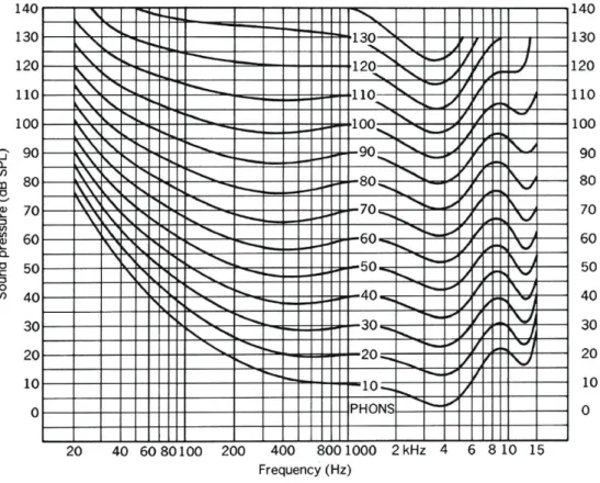
Loudness is the subjective perception of the sound intensity and is related to Sound Pressure Level, frequency content, and duration of the signal. The sensitivity of human auditory system changes as a function of the frequency and not only as a function of the SPL as shown in the plot 3.1. The figure 3.1 shows the diagram of Fletcher and Munson and two main thresholds can be detected. The hearing threshold indicates the minimum sound level

(29)

perceivable to the human ear. The pain threshold represents the maximum sound level that a human ear can perceive without feeling pain. The other lines, called isophonic curve, show the SPL required for each frequency to be perceived at the same loudness. We can also observe from the diagram that the ear was thought to perform at its best in the speech range between 1 kHz and 4 kHz. However, it has a minimum perceivable pitch of 20 30 Hz while a maximum of 15-20 kHz.

In the Fletcher and Munson diagram the Loudness Level is also indicated, expressed in Phon, for each isophonic curve at 1 kHz.

Figure 3.1: Fletcher Munson diagram

(30)

3.1.3 Timbre

In a situation where two sounds have identical pitch, loudness, and duration, they could not be distinguished but thanks to the timbre character they can be. Timbre is a general character of a sound, usually attributed to the sound of an instrument. It denotes a digital fingerprint of all the sounds of an instrument.

From the Acoustical Society of America, the Acoustical Terminology defines the timbre as ”that attribute of auditory sensation which enables a listener to judge that two nonidentical sounds, similarly represented and having the same loudness and pitch, are dissimilar. The timbre depends primarily upon the frequency spectrum, although it also depends upon the sound pressure and the temporal characteristics of sound” (Acoustical Society of America Standards Secretariat 1994).

The timbre is used to define the color or the quality of the sound. It is closely influenced both by the time evolution (attack, decay, sustain, release time) and by the spectral components in a sound.

3.1.4 Rhythm

The temporal relation between events is described by the rhythm. The per-ception of it is linked to two different factors: the grouping, which is more formal measure, whereas the meter, is a more perceptive one. Indeed, group-ing refers to hierarchical division of a musical signal in the rhythmic struc-tures of variable length.

A group can be extended from a set of notes to a musical phrase to a musical part. On the other hand, meter refers to regular alteration between a strong beat and a weak beat heard by the listener. Pulses or beats do not have an explicit assignment in the music but are induced by the observation of a rhythmic pattern underlying the musical structure.

The main measure to define the rhythm of a song is the tempo. Tempo de-fines the rate of the most prominent among the pulses and it is expressed in Beat Per Minute. Indicating with Tactus the beat, i.e. the measured tempo reference for each individual event, the Tempo can be expressed as the time rate of the Tactus. The shortest time interval between events in the track is called Tatum and constitutes the base structure of it. Finally, bars refer to harmonic changes and rhythm pattern changes. The number of beats in every measure is called time signature.

(31)

3.2 Music information retrieval

Music Information Retrieval (MIR) is ”a multidisciplinary research endeavor that strives to develop innovative content-based searching schemes, novel in-terfaces, and evolving networked delivery mechanisms in an effort to make the world’s vast store of music accessible to all”, as defined by Downie [42]. The quote of Downie is explicative of the wideness and of the potential that the Music Information Retrieval has in today’s world. Due to the increasing number of streaming services and the consequent availability of mobile music, the interest concerning the Music Information Retrieval is quickly increasing. It is mainly focused on the extraction and the inference of meaningful features from music, on the indexing of music, and on the development of the scheme for the retrieval and the research of data. Of particular interest during this work are those MIR applications referred to feature extraction. Indeed, in the case of Automatic Music Transcription methods, descriptors of audio signals play a central role in understanding musical contents. In fact, AMT systems can be decomposed as MIR tasks linked to mid-level features. Note onset and offset detection, beat tracking or tempo estimation represent the actual research field needed for a complete transcription.

Onset detection has the aim to identify the start point of an event, called on-set. More specifically the onset detection needs to identify the starting point of all the events within a musical signal. Depending on the instrument being played, onsets can be divided into three categories: pitched, percussive or pitched-percussive. The first is typical of string instruments or wind instru-ments; percussive ones are produced by drums; finally, pitched-percussive onsets characterize instruments such as the piano or guitar.

Facing polyphonic music with multiple voices complicates the onset task, since every voice has its own onset characteristic. Furthermore, onsets can be modified for aesthetical purposes using musical effects like the tremolo and the vibrato or other audio effects. Usually, modifications constitute interfer-ences in the onset detection task. For this reason, there are some methods focused on the onset detection suppressing vibrato like the one proposed by B¨ock [34].

Metrical organization of musical tracks follows hierarchical structure from the lower level, the beat, to the higher one, the time signature. The beat is the reference for each musical event and constitutes the most important rhythmic element. A pre-stated number of beats form a bar, the number of

(32)

the beats that need to be present in a bar is indicated by the time signature or meter. On the other hand, downbeats are meant to be the first beat inside a bar and it can be linked to rhythmic patterns or harmonic changes within a musical piece.

Linked to the beat tracking, the tempo estimation task has the aim to recog-nize accurately the frequency at which beats occurs. Although theory could suggest deriving the tempo of a musical piece from the beat estimation, which is not as easy as it might appear. Tempo hypothesis is needed for a robust and good beat estimation algorithm.

3.3 MIDI

MIDI, which stands for Music Instrument Digital Interface, represents a com-munication digital language. It works with specifics that make possible the communication between different devices inside a cabled network. Finally, the MIDI is a medium to translate events linked to a performance or a con-trol parameter, such as pressing a key on the keyboard. Those messages can be, then, transmitted to other MIDI devices or can be used later on after the recording.

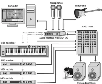
Figure 3.2: MIDI network scheme

A basic device within the MIDI environment is the sequencer. A MIDI sequencer can be software or hardware, which is used to record, modify and

(33)

send to the output MIDI messages in a sequential way. The MIDI messages are usually divided per track, each one dedicated to a different instrument as required by the producing concept. MIDI Tracks contain events and messages working on a specific channel. Once the performance has been recorded, it is stored and can be arranged or modified also with the help of graphical in-terfaces depending on the sequencer. Data is then stored in a file or a digital audio workstation to be played back or reused in different ways.

Most used sequencers are the software ones due to their portability through different Operating Systems. They exploit the versatility, the calculus speed and the memory of a personal computer.

From an artistic viewpoint, thanks to its flexibility, the MIDI language is a really important medium for artists. Once the MIDI has been recorded and mastered it can overtake the analogic difficulties and the recorded per-formance can be edited and controlled. In this dissertation, exploiting the power of the standard, we will use the MIDI annotation to use different pi-ano or instrument sounds on the same performance in order to have more variability inside the dataset.

It is important to remember that the MIDI does not have inside itself any sound information and does not communicate any audio waves or create any sound. It is a language to transmit instructions to devices or programs to create and modify the sound. This is the great strength of the MIDI standard since it permits the files to be very lightweight.

A Standard MIDI file can be of three formats:

1. Format 0: all the tracks of a song are merged in a unique one containing all the events of all the tracks of the original file;

2. Format 1: tracks are stored separately and synchronously, meaning that each track shares the same tempo value. All the information about tempo and velocity of the song are stored in the first track, also called Tempo Track. It is the reference point for all the other tracks; 3. Format 2: tracks are handled independently also for the tempo

man-aging.

Within a MIDI track, every event is divided from other events by temporal data called Delta-time. Delta-time translates into byte, the time between two occurring events, so it represents the duration in Pulse Per Quarter Note between an event and the following one. PPQN is the duration in a

(34)

microsecond of an impulse or also called tick per a quarter of note. It is given by the following equation: 60000000/bpm_{P P QN} . The Beat Per Minutes represents the metronome time of the song, while the PPQN is the resolution in impulses for a quarter of a note.

3.3.1 MIDI messages

The medium for the communication between devices within the MIDI net-work is called MIDI messages, transmitted along serial MIDI lines at 31,250 bit/sec, where MIDI cable is unidirectional. Data in a serial line follow a unique direction in a conductor cable, while in a parallel line data can be transmitted simultaneously to all the devices connected.

In MIDI messages the Most Significant Bit, left one, is dedicated to identi-fying the kind of byte. Bytes of MIDI messages could be Status Byte if the MSB is set to 1, or Data Byte if MSB is set to 0.

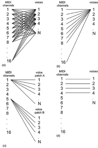
To permit different kinds of connections between devices and different in-struments, guidelines were specified, following those specifications a device can transmit or respond to messages depending on its own internal settings as specified in the figure 3.3. As a matter of fact, there is a different mode in which an instrument can work. The Base Channel is an assigned channel and determines which channel the device would respond to.

Now we will take a deep view of the mode in which a MIDI device can work: • Mode 1: Omni mode On, Poly mode On, the instrument will listen to all channel and retransmits the messages to the device set at the Base Channel. In this mode, the device acts as a relay of input messages in a poly mode. It is rarely used.

• Mode 2: Omni mode On, Mono mode On, the instrument will listen to all the channel and retransmits the messages to the device or instrument set at the Base Channel, the latter can act just as monophonic device. In this mode, the device acts as a relay of input messages in a poly mode. It is even rarer than the Mode 1 since the device cannot detect the channel nor play multiple notes at the same time.

• Mode 3: Omni mode Off, Poly mode On, the instrument would respond just to the assigned Base Channel in a polyphonic fashion. Data from a different channel from the Base Channel would be ignored. It is the most common mode due to the fact that voices within the multitimbral

(35)

device are controlled individually through messages on the channel, reserved for that voice.

• Mode 4: Omni mode Off, Mono mode On, the instrument would lis-ten to the assigned Base Channel, but every voice is able to play a unique note per time. A really common example is the recording sys-tem for a guitar, where each data is transmitted in a monophonic way on one channel, one for each string, as a matter of fact, one cannot play multiple notes on a single guitar string.

Figure 3.3: Voice channel assignment of the four modes that are supported by the MIDI: top left Omni on/poly; top right Omni on/mono; bottom left Omni off/poly; bottom right Omni off/mono

(36)

Channel voice messages

Channel voice messages are used to transmit real-time performance data through a MIDI cabled system. Every time a parameter or a controller of a MIDI instrument is used, selected or changed by the performer, a channel voice message is emitted. Below are specified some of the most used channel voice messages:

• Note-On: used to denote the start of a MIDI note, it is generated every time a key is triggered on a keyboard, a controller or on other instruments. Status Byte contains the Note-On status and the midi channel number; Data Byte to specify which of the 128 MIDI pitch note needs to be played, one Data Byte to denote attack velocity of the pressed key or the pressure, the volume of the note is affected by the latter. MIDI note is contained in the interval from 0 to 127 knowing that in position 60 is placed the C4, to give an example the keyboard has 88 keys and its MIDI note interval comprehends numbers from 21 to 88. In the specific case in which a note has an attack velocity 0, the On events is equal to a Off. This peculiar use of the Note-On message was exploited in the project to modify easily the MIDI files without deleting any of the events.

• Note-Off: is the message to stop a specified MIDI note. The sequence of MIDI events is characterized by a sequence of Note-On Note-Off messages. The note-off command would not cut the sound, but it would stop the MIDI note depending on the release velocity parameter that represents how fast the key was released.

• Program-change: it is a message for specifying a change in the number of the program or pre-set which is playing. The program number usu-ally define the MIDI instrument to play, pre-sets are usuusu-ally defined by manufacturers or by the user to trigger a specific sound patch or a specific setup.

• All Notes-Off: since a MIDI note could remain played, All Note-Off message can be used to silence all the modules that are playing. • Pressure/Aftertouch: it renders the double pressure on a key.

(37)

• Control-change: it is used to transmit information related to changes in real-time control or performance parameters of an instrument like foot pedals, pitch-bend wheels.

3.3.2 System messages

System Messages are forwarded to every device within the MIDI network, so there is no need to specify any MIDI channel number. Every device would respond to a System Message. Three are the types of System Messages in the MIDI Standard:

1. System Common Messages: they transmit general information about the file being played like the MIDI time code, the song position, the song selection, the tune request. Typical System Common messages are: MIDI Time Code Quarter-Frame,Song Select, End of Exclusive messages;

2. System Exclusive messages: are special messages left to the manufac-turers, programmers, and design to make other devices of the same brand communicate without restriction of the length of data and MIDI messages customized;

3. Running Status messages: running status messages are a special type of messages used in a situation of redundancy of the same type of message. It permits a sequence of the same message type to omit the Status Byte, that would be the same for each one. If for example, we have a long series of Note-On messages on a specific channel with a Running Status message, we can omit the Status Byte.

(38)

3.4 Introduction to machine learning and

Neu-ral Networks

Nowadays, artificial Intelligence, AI, is widely used in many research areas not only automating routines but also in the field of discerning high-level of information. The true challenge for artificial intelligence was solving those tasks hardly describable for people due to their spontaneous and intuitive nature.

The Deep Learning term is linked to that way to approach an AI problem in which tasks requiring high-level concepts need to be decomposed in many lower-level terms [24].

One of the main reasons for the increasing use of deep learning in the last 20 years was the growing quantity of digitalized data. Training data is really important in deep learning. The process of digitalization of the society and the consequent start of the era of Big Data makes easier the resolution of Machine Learning problems. Indeed, Machine Learning algorithms end with good results when trained on a big amount of data.

Neural Networks are a framework to approach Machine Learning problems. They take inspiration from the human brain system: how it is composed, how it is connected and how its elements interact with each other.

Artificial Neural Networks are composed of interconnected processing units. The goal of the network is to find an approximated function f∗ that can map the input x as the target y. ANN try to minimize the result of the function f∗ so to have y = f∗(x). The processing units are also called artificial neu-rons of the network and they usually perform a sum on the weighted inputs they receive. The weight of each input depends on how much the input influ-ences the neuron. The output of the weighted sum, called activation value, is usually modified by a bias value which is then passed as input to a transfer function.

The transfer function σ(a) applied to the activation value calculated by the neurons is a non-linear function like a hyperbolic tangent, arc-tangent, and sigmoid. σ(a) =        1

1+e−a, sigmoid

tanh a, hyperbolic tangent max(0, a), ReLu

(39)

Additional non-linearities can be added depending on the purpose of the Neural Networks, for example, the softmax algorithm can be applied to clas-sification problems.

The topology of a network refers to the way in which neurons are connected among each other to accomplish for example a pattern recognition problem. Usually, Neural Networks are organized following a layered structure. In each layer, the set of all the activation values from each neuron is called the activation state of the network, while the output state is the set of all the neurons’ output related to a layer.

The training of the Network consists of adjusting the parameters of each neuron, weight and bias, in order to get an approximation of the output as close as possible to the desired output target, provided by the input data at the Network. Thanks to the layered structure, an iterative algorithm can be used during the training, such as the backward propagation of the error based on the gradient descent method. The gradient is the loss function and measures the difference between the real output of a neuron and its desired target output. Depending on the results of the gradient loss, the parameters of the neurons are updated to get the minimal error between the target and the actual output. Different loss functions are available for calculation such as cross-entropy function, the one chosen during the development of the NN used within the AMT system.

The minimization of the loss during the training phase can be performed in three different approaches. Batch Gradient Descent approach tries to min-imize all the sets of data. Stochastic Gradient Descent applies single data to the Neural Network. Finally, Mini-Batch Gradient Descent use just a little subset for the training. In addition, to avoid problems such as local minima and to accelerate the training process, optimized Gradient Descend algorithms were developed like Nesterov, Adam, Adadelta or RMSprop [24]. The activation state of a network represents the activation values in a layer and determines the short-term memory of a network. On the other hand, long-term memory is represented by the learning process of adjusting weights [24].

(40)

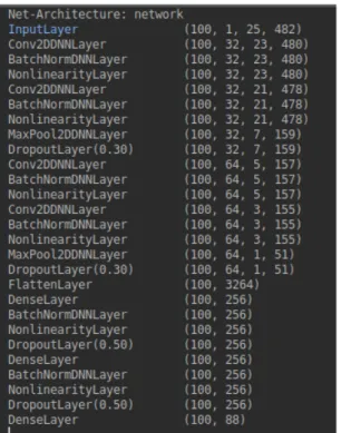
A variant of Forward Neural Networks is the Convolutional Neural Net-work, figure 3.4. Its main characteristic is the fully connected convolutional layer. CNN was chosen in the dissertation as framework for the pitch detec-tion task.

Figure 3.4: Convolutional Neural Network scheme

The extension of basic Neural Networks exploits the long and short corre-lation of the input signal with different types of Networks. Recurrent Neural Networks, figure 3.5, for examples, extend Forward Neural Networks with feedback connections, allowing the connection of previous layers. Feedback connection accounts for different time instant of the input relating the actual input to the past one, representing short time memory.

Figure 3.5: Deep Neural Network scheme. Left: Forward Neural Network; Right: Recurrent Neural Network

(41)

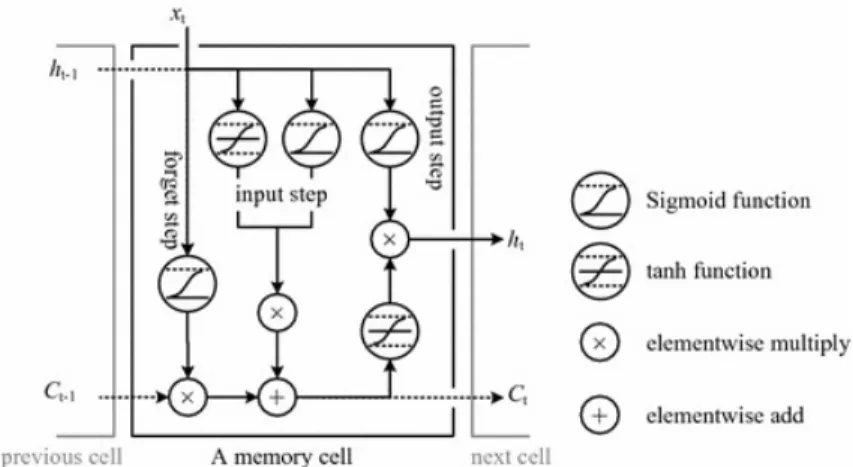
Long-term memory is exploited with the use of Long-Short Term Memory cells, figure 3.6, allowing the Neural Network to learn long-term dependen-cies. LSTM cells have an internal memory that can be accessed and updated from gates depending on the input they are fed with.

Figure 3.6: Long Short-term cell

3.5 Madmom library

Due to the emerging of the Music Information Retrieval research field in recent years, audio-based systems for the retrieval of valuable information have become more important. Furthermore, their role is still gaining rele-vance thanks to the increasing trend of available data.

Audio-based MIR systems in the state-of-the-art are designated as systems which make use of low-level feature analysis for retrieving meaningful mu-sical information from an audio data. The latest audio-based MIR systems exploit Machine Learning algorithms to extract this information. Further-more, they usually integrate a different level feature extraction sub-system to derive them directly from the audio signal.

Madmom library, as an open-source library, was thought to facilitate research in MIR field both in terms of low-level feature extraction, like Marsyas and YAAFE, and in terms of high-level extraction like MIRtoolbox, Essentia or LibROSA. What makes Madmom different from all the other libraries is the use of Machine Learning algorithms [34].

Madmom library would like to give a complete processing workflow allowing

(42)

the construction of both full processing systems and stand-alone programs using Madmom functionalities. Thanks to Processors objects, Madmom con-verts running programs into a simple call interface.

The use of Processors allows an easy use of complicated and long proce-dures included in the library as low-level feature extraction ones. High-level features are then used by Machine Learning techniques to retrieve musical information. Madmom includes both Hidden Markov Model and Neural Net-work methods applied to state-of-the-art algorithms of MIR tasks as onset detection, beat, and downbeat detection, and also meter tracking, tempo estimation and chord recognition. Availability of state-of-the-art techniques permits users to build a complete processing method or just integrate them in stand-alone programs as we have done.

Madmom is an open-source audio processing and Music Information Re-trieval library based on Python language. Following the Object Oriented Programming approach, it encapsulates all the information within objects that instantiate subclasses of the NumPy class.

Madmom depends just on three external modules: one for array handling routines, NumPy, one for the optimization of linear algebra operation for FFT, SciPy, and finally one for the speed-up of critical parts, Cython. ML algorithms can be applied without any other third-party modules since they are algorithms pre-trained on external data, which are just tested with input data, allowing reproducible research experiments.

The source code for each file is available on the net and the complete docu-mentation for the API can be found at http://madmom.readthedocs.io. The Madmom library was extensively employed during the development of the Automatic Music Transcription system. In particular during feature extraction and peak detection phases (the latter applied during the pitch detection). It was exploited for its robust algorithms, and is easy to include within external code.

(43)

Chapter 4 Methodology

The proposed transcription system consists of three main phases as suggested from the figure 4.1: an initial signal-processing stage, followed by an activa-tion funcactiva-tion calculaactiva-tion and finally a peak picking one. In the first phase features are extracted from the audio signal and target values are also de-rived from the MIDI files. Feature extraction works on raw audio data, while target creation works on that of MIDI. During the activation function calcu-lation phase, the Neural Network is trained on the same input features. The final stage is represented by the detection of onset employing a simple peak picking method. After the training of the Neural Network, the evaluation phase consists of the prediction extraction from the interpretation of the fea-tures. Target and evaluation prediction are compared to estimate the system.

(44)

The following sections describe the entire system workflow, narrowing down the analysis to the signal processing and the Neural Network training phases that can be referred to as the core of the method itself.

4.1 Design choices and considerations

Automatic Music Transcription systems aim at retrieving a new represen-tation of the input signal starting from a different one, exploiting analysis methods. The Dixon method, for example, uses a time representation of the signal. But, usually, as seen throughout the relevant section 2.4, probabilistic and factorization algorithms rely on a time-frequency one. One of the main reasons which support the choice of undergoing through time-frequency anal-ysis, the method employed to perform our study, is the simultaneous study of a signal under both time and frequency parameters. In fact, their tight coupling helps and supports the signal analysis. From a practical point of view the signal can be transformed from a one-dimensional signal to a two-dimensional one through the Fourier Transform, assuming the signals to be either infinite in time or periodic. A more realistic interpretation of the Fourier Analysis is the Short-Time Fourier Transform used to compute the Fourier Transform on short time-frames. STFT determines frequency con-tent and phase in each local time-frame and was the one chosen in the dis-sertation. Other time-frequency representations are available for analyzing the signal like Q-transform, Wavelet transforms and Bilinear time-frequency distribution. In practice, Short-Time Fourier Transform and Q-Transform are the most frequently employed ones due to the availability of convenient computational algorithms and deep theoretical knowledge. STFT’s main drawback is constant frequency resolution, which may generate problems an-alyzing lower frequencies. To overcome this issue, usually, a bank of filters of a number of pitches is used (12 per octave in the case of musical signals) with all the filters logarithmically spaced. Indeed the Q-Transform can be seen as a logarithmic-spaced filter to which Fourier Transform is applied. In the case of multi-pitch system, the evolution in time of the spectral con-tent of a signal is really important to understand. Furthermore, the pitch being played is extracted from the frequency content, and the onset time of a note from the time information.

An investigation of piano transcription algorithm for jazz music

POLITECNICO DI MILANO

AN INVESTIGATION OF PIANO

TRANSCRIPTION ALGORITHM

FOR JAZZ MUSIC

Supervisor: Prof. Fabio Antonacci, Politecnico di

Milano

Co-supervisor: Prof. Peter Knees, Technische

Universit¨

at Wien

Co-supervisor: Richard Vogl, Technische Universit¨

at

Wien

Master Thesis of:

Giorgio Marzorati, ID 876546

Abstract

Acknowledgment

Contents

List of Figures

List of Tables

Chapter 1

Introduction

1.1

The challenge of Automatic Music

Tran-scription

1.2

Scope of the thesis

1.3

Aims and applications

1.4

Structure of the thesis

Chapter 2

Related works

2.1

Overview on Automatic Music

Transcrip-tion

2.2

Automatic Music Transcription history

2.3

Single-pitch estimation

2.4

Multi-pitch estimation

2.4.1

Signal processing techniques

2.4.2

Statistical techniques

2.4.3

Spectrogram factorization techniques

2.4.4

Machine learning techniques

2.5

Trend and future directions

Chapter 3

Background and terminology

3.1

Musical sounds

3.1.1

Pitch

3.1.2

Loudness

3.1.3

Timbre

3.1.4

Rhythm

3.2

Music information retrieval

3.3

MIDI

3.3.1

MIDI messages

3.3.2

System messages

3.4

Introduction to machine learning and

Neu-ral Networks

3.5

Madmom library

Chapter 4

Methodology

4.1