Testing crucial model assumptions: the income/willingness to pay for the environment nexus in the Environmental Kutznetz Curve
Abstract
Several theoretical models investigating the relationship between economic growth and environmental degradation postulate that consumers’ willingness to pay for it gets higher as far as per capita income grows. We test this hypothesis on willingness to pay (WTP) for the environment data collected from the World Value Survey database for a large number of countries and find strong support for it after controlling for demographics, personal values and country variables such as domestic institutional quality and pollution intensity. We also document that the additional and most robust determinants of the WTP are age, education, religious practice, proxies of civic values (tax morale, sense of belonging to a wider community) and quality of domestic institutions.
Sabrina Auci
University of Rome Tor Vergata Leonardo Becchetti
University of Rome Tor Vergata Luca Rando
University of Rome Tor Vergata
1. Introduction
The Environmental Kuznets Curve (EKC) hypothesis postulates the existence of an inverse U-shape relationship between per capita GDP and measures of environmental degradation (Panayotou, 1993 and 2000; Grossman and Krueger, 1991 and 1995; Selden and Song, 1994; Shafik and Bandyopadhyay, 1992; Hettige, Lucas and Wheeler, 1992, Koop, 1998, Stern 2004; Copeland and Taylor, 2004).
According to the EKC literature such relationship may be determined by a series of concurring supply and demand side factors such as: i) economies of scale in pollution abatement, ii) changes in the industry mix and evolution from physical to human capital intensive activities, iii) changes in input mix; iv) changes in the elasticity of income to the marginal damage generated by environmental degradation; v) changes in environmental regulation (Stern, 2004; Copeland and Taylor, 2004).
Early EKC empirical models, with a few exceptions, share the limit of being built on heuristic theories or ex post theoretical justifications of their findings rather than ex ante formal derivations from individual optimizing behaviour (Panayotou, 2000). More recently, however, a wide range of theoretical models have been developed whose results are broadly consistent with the findings of the empirical literature.
Each of these models focuses on specific mechanisms from which the inverted U-shape relationship may be derived. Lopez (1994) and Selden and Song (1995) provide an overlapping generation framework with exogenous technological growth, in which pollution is generated on the supply side. Brock and Taylor (2004) show that, once technological progress in abatement is incorporated into a Solow exogenous growth model, the EKC is a necessary by-product of convergence to a sustainable growth path. John and Pecchenino (1994), John, Pecchenino, Schimmelpfennig, and Schreft (1995), and McConnell (1997) focus on demand side determinants. Finally, Copeland and Taylor (2004) show that the EKC may be solely generated on the demand side when the
government maximizes the utility of a representative consumer and the latter has an elasticity of income to the marginal damage suffered from pollution, which varies in the level of income, or is subject to some threshold effects.
The consumption side changing elasticity of income hypothesis has therefore a crucial role in the EKC literature but has seldom been tested. The first relevant attempts come from Israeli and Levinson (2001), Ivanova and Tranter (2005) for Australia and Garcia and Togler (2005) for Spain.
Our study aims to test this hypothesis and differs from the previous ones in several respects: i) we outline in a microfunded theoretical model the theoretical link between the inverse U-shape of the EKC and the changing elasticity of income hypothesis; ii) we decompose the impact of income into absolute and relative effects; iii) we use a richer set of variables at individual level, controlling not only for standard demographics (education, age, gender and town size), but also for individual values (sense of belonging to a wider community, tax morale, national proudness, etc.) and for country variables related to pollution intensity, institutional quality and tax pressure.
The paper is divided into five sections (introduction and conclusions included). In the second section we sketch the theoretical framework outlining the link between the shape of the EKC and the relationship between per capita income and the willingness to pay for the environment which we are going to test. In the third section we illustrate characteristics of the database and our descriptive empirical findings. In the fourth section we comment econometric findings. The fifth section concludes
2. The theoretical framework for a consumer driven environmental Kutznets curve
To illustrate the relevance of our empirical analysis, and to highlight the role of consumer preferences in the EKC literature, we illustrate the general equilibrium framework presented by Copeland and Taylor (2004) and show that, in this framework, the inverse U-shape of the EKC may be solely determined by the changing elasticity of income hypothesis. We further explain how our empirical analysis represents a direct test of this hypothesis.
In the supply side of the Copeland and Taylor (2004) model there are two goods (X and Y) produced with constant returns to scale, where p is the price of product X and product Y is the numeraire. The authors assume that the productive process of X generates pollution, while the same does not occur for Y.
Pollution is considered as an input (but the model may be represented equivalently by considering it as a joint output) in the following production function
1
[ ( x, x)]
x = zα F K L −α
where x is the output of product X, z is pollution, F(.) is the production function of good X, K and L are the usual production inputs (capital and labour) and 0<α <1. The government sets a price τ for each emission unit and, due to the Cobb-Douglas functional form, emission costs on total output are α=τz/px. The interior solution of the firm which minimizes emission intensity is equal to e=z/x= α/pτ. With non positive profits and full employment it is possible to derive output functions of the type x=x(p,τ,K,L) and y=y(p,τ,K,L) for the two goods.
In the model the private sector maximizes national income for a given pollution level z G(p,K,L,z)=
{ },
{
}
max : ( , ) ( , , ) x y px+ y x y ∈T K L z
with T being the feasible technology set. In this framework it is possible to demonstrate that, in equilibrium, the price of pollution (τ) is equal to the value of the marginal product of emissions. In the Copeland-Taylor (2004) model the economy is populated by identical consumers with the following indirect utility function V(p,I,z)=v(I/β(p))-h(z), where I stands for per capita income, β is a price index, h’>0, h’’>0, v’>0 and v’’<0.
From the model it is possible to derive the following corporate demand for pollution, z= α(p/τ)x(p,τ,K,L), which is downward sloping in the (τ,z) space.
Pollution supply is chosen by a benevolent planner who can obtain exactly the target level of emission z0, either by imposing it, or by choosing the price τ0 such that the horizontal supply of
emissions crosses the downward sloping demand curve in z0.
The more reasonable assumption, though, is that the benevolent planner does not act as a dictator, but maximizes the following indirect utility function of the representative consumer
{ }
{
}
max V(I/ (p),z)s.t.I=G(p,K,L,z)/N
z β .
If the economy is small, and p is given, the first order condition will be 0 I z z V G V N + = .
By rearranging this first order condition it is possible to obtain the following upward sloping supply of pollution
[
]
* Z / I * ( , , )
N V V N M D p R z
τ = − =
where R=I/β is real income and MD is the consumer’s marginal damage from pollution, or the marginal rate of substitution between pollution and income.
By setting demand of pollution equal to supply we obtain the market clearing equilibrium level of emissions
( , , , ), ) * ( , ( , , , ), )
z
G p K L z z = N M D p R p K L z z .
At this point the authors evaluate the effect of a neutral technological progress shift λ. The shift moves demand to the right and supply to the left since
( , , , ), ) * ( , ( , , , ) / ( ), ) z G p K L z z N M D p G p K L z p z λ = λ β . Given that dz 1 M D R, d ε λ − =
∆ , we know that the new equilibrium level of pollution on the horizontal axis will be lower than before if the income elasticity of the marginal damage is higher than one. Hence, as far as per capita income rises, if the above mentioned elasticity grows and passes from less to more than one, we obtain the classical inverse U-shaped pattern of the EKC.
To provide an example with a specific functional form, in order to have an EKC generated by a pure income driven explanation, we need an indirect utility function of the type
/
1 2
V(p,I,z)=c R ( )
c e− ξ h z
− − .
In such case, the income elasticity of the marginal damage from pollution is R/ξ and, therefore, as far as real income grows and moves from R<ξ to R>ξ, we obtain the inverse U-shaped pattern of the EKC.
2.1 The model and our empirical test
Consider now the relationship between our empirical test and the Copeland-Taylor (2004) model. In the empirical section we test whether the willingness to pay grows in income quintiles, net of all the other possible country effects and of the impact of other control variables. If we have coefficients of income quintiles that are increasing and positive after some income quintile threshold (and if the magnitudes are significantly different at a given distance among quintiles), we definitely demonstrate that the willingness to pay for the environment grows as far as income gets higher.
Consider also that a passage from a zero to a nonzero willingness to pay for the same individual must be necessarily related to an increase in the income elasticity of marginal damage since the ratio between the disutility of pollution and the utility of income must necessarily rise to obtain this result.
Nonetheless, our result does not exactly coincide with the assumption of the model, where the representative consumer (the same individual) is modeled as having an income elasticity of marginal damage which grows in real income. To what extent is our finding close to what the model assumes and, under what conditions may we conclude that it produces equivalent results ?
Consider that we will try to control for all possible covariates in our econometric estimate. This is important as we isolate the income effect from all other possible concurring effects which may have an impact on the willingness to pay for the environment. The richer our set of controls, the more confident we are that we are measuring the true willingness to pay-real income relationship.
Second, what our result exactly tells us is that, coeteris paribus, a higher share of individuals will be willing to pay something for the environment when we move up across income quantiles.
If we aggregate all our respondents into a representative individual, and translate the share of those who are willing to pay for any given income quantile into a measure of the amount of the willingness to pay of the representative consumer, we have a relationship which is correspondent to the one described in the model.
Hence, under the reasonable assumption of a one to one mapping from i) the share of those willing to pay in a given income quintile into ii) the income elasticity of the marginal damage of the representative individual, we may establish an equivalence between our finding (coeteris paribus, at higher income quantiles more people are willing to pay for the environment) and the model assumption (the representative consumer has an increasing income elasticity of marginal damage as far as real income rises) which is crucial to obtain a pure consumption driven EKC.
3. The database and the descriptive evidence
We test our hypothesis on the cross-sectional database of the World Value Survey which joins representative samples from more than 60 countries in the world1
The two questions related to the WTP for the environment, relevant for our empirical work, are the following: i) I would agree to an increase in taxes if the extra money were used to prevent environmental damage (in WVSs 1990–1993 and 1995-1997), I would agree to an increase in taxes if the extra money were used to prevent environmental pollution (in WVS 2001); ii) I would give part of my income if I were certain that the money would be used to prevent environmental pollution (in WVS 2001).
As it is well known, the literature on contingent valuation highlights some potential biases arising from the investigation of the willingness to pay for a given good based on a direct demand on it from survey data (Mitchel-Carson, 1989; Diamond-Hausman, 1994). A first bias is represented by strategic behaviour when the respondent knows that his response may affect the decision on the quantity of a public good and service provided. A second bias arises when the hypothetic scenario prospected by the interviewer is too unrealistic. This bias may be reduced if the respondent is familiar with such scenario. A third bias is the so called “embedding effect”. Many empirical results
1 The World Values Survey is a worldwide investigation of sociocultural and political change. It has carried out representative national surveys of the basic values and beliefs of publics in more than 65 societies on all six continents, containing almost 80 percent of the world's population. It builds on the European Values Surveys, first carried out in 1981. A second wave of surveys, designed for global use, was completed in 1990-1991, a third wave was carried out in 1995-1996 and a fourth wave took place in 1999-2001. The surveys are based on stratified, multistage random samples of adult citizens aged 18 and older. Each study contains information from interviews conducted with 300 to 4,000 respondents per country.
(see, among others, Kahneman-Knetsch, 1992; Carson et al. 1995; Randall-Hoehn, 1996) show that quantitative responses tend to be strikingly similar, in spite of the different situations presented within the same scenario. The rationale is that individuals have a clear idea of their general WTP for a given good, but not of its exact quantitative amount and of its variation according to changes in the side conditions prospected in the hypothetical demands. As a consequence, they tend to round up or to converge to average values. The fourth is an upward bias on WTP findings generated by the desire of the respondent to please the interviewer when it is costless to do so.
By looking at the WVS questions we may conclude that the first bias might lead to an underestimation of the willingness to pay for the environment, provided that some individuals who care for it believe that their answers might have economic consequences and want to free ride to shift the burden on other respondents. With regard to the second bias, paying more taxes for the environment does not appear to be particularly unrealistic and therefore this distortion should not be significant.
The third bias should not apply since all of the three questions carefully avoid to ask respondents to quantify exactly their willingness to pay. The fourth bias should not apply as well since the questionnaire has a large number of questions on different issues concerning values and it is difficult to figure out that the interviewer desires a positive response on the two questions above. Consider finally that a fifth bias (similar but not identical to the fourth) might apply since respondents are generally inclined to provide a positive image of themselves when there are no costs for doing it. This is likely to induce to an overestimation of the willingness to pay. In support of this hypothesis we may observe a gap between the declared willingness to pay, on the one side, and, on the other side, the revealed preferences of consumers toward green or “socially responsible” products whose market shares are far below those implied by willingness to pay answers.2 Part of this difference, though, may be explained by the fact that consumer choice occurs in reality in a framework of imperfect information on the environmentally responsible characteristics of the products and that (due to the presence of a limited range of environmental products) consumers seldom have the opportunity to choose without differences in search costs between two identical products, differentiated only on the basis of the environmental friendly characteristics.
To conclude on this point, consider however that the focus of our paper is not on the evaluation of the exact share of respondents who declare a willingness to pay for environmental quality, but on the determinants of the latter and, more specifically, on the difference in the impact on our dependent variable of different income classes, net of all relevant control factors. We may therefore reasonably assume that such difference should not be affected by the above mentioned possible distortions on willingness to pay responses. This is likely to be true under the non particularly restrictive assumption that the desire to please the interviewer is uncorrelated with income.
3. 1 Descriptive evidence
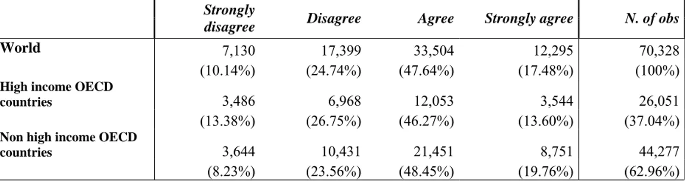
Descriptive evidence shows that around 17 percent of respondents would strongly agree (and around 48 would agree) to an increase in taxes when the latter are used to prevent environmental damage (Table 1).3 The share is surprisingly lower for high income than for non high income
countries, most of them being emerging countries (14 percent against 20 percent would strongly agree and 46 against 48 would agree). Remember, though, that what we are measuring here is the
2 Information on market shares of green and socially responsible products in different countries may be found, among others, from Demos & Pi / Coop (2004) for Italy, Moore (2004) and Bird and Hughes (1997) for the UK, De Pelsmacker, Driesen and Rayp (2003) for Belgium and TNS Emnid for Germany (www.fairtrade.net/sites/aboutflo/aboutflo).
3 Note the slight difference in the tax question between the 1990-93 and 1995-1997 WVSs (taxes used to prevent environmental damage) and the 2001 WVS (taxes used to prevent environmental pollution). In Table 1 we pool information from these two questions while in the econometric analysis country dummies will control for time effects and therefore for differences in demand formulation.
“excess demand” of environmental protection, that is, the demand not already covered by domestic environmental policies. In this perspective, it may be reasonable to assume that the willingness to pay extra taxes for environmental protection may be lower in countries in which environmental policies are already well developed.
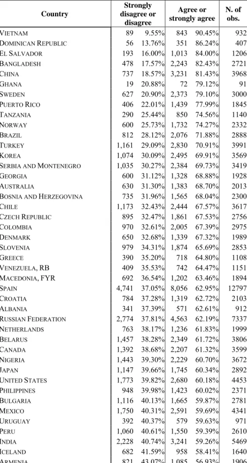
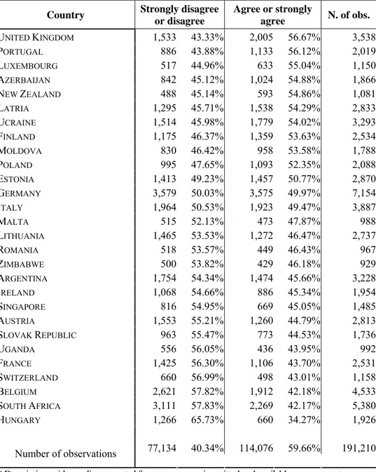
Keeping this in mind, we look at descriptive evidence on country rankings (Tables 2A-2B) and observe some findings which are expected (countries such as Sweden and Norway are among the first ten in terms of the willigness to pay more taxes, Eastern European countries are almost all on the bottom of the ranking) and some others that may be puzzling (why Vietnam and some Central American countries are on the top ?). Country rankings on the willingness to give part of the income question are substantially similar (Table 2B). To interpret these descriptive findings consider that country differences may be affected by sample composition effects related to the factors which affect the willingness to pay for the environment and that there may be some relevant cultural differences in the way interwieved individuals declare their willingness to pay (most Asian countries are for example on the top, and Eastern European countries are at the bottom, in the same World Value Survey in terms of tax morale). In the rest of the paper we will not focus on country differences and take into account the problem of cultural disparities by controlling with country dummies our test on the relationship between the dependent variable and individual income.
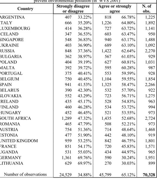
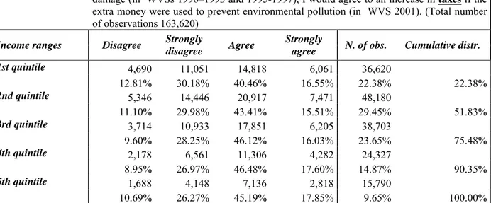
Descriptive evidence on the relationship between the willingness to pay for the environment (in terms of payment of higher taxes or destinatition of part of the respondent’s income) and progression across income quintiles seems to indicate a significant link between the two variables in the tax question (Tables 3A-3B), even though when we aggregate disagreement and agreement (regardless of the intensity) we do not find a monotone relationship across quintiles. The sum of the shares of those who agree and strongly agree is at 57 percent in the first quintile and goes monotonically up to 64 percent in the fourth quintile (but it slightly falls to 63 percent in the last). The relationship appears stronger in the income question (Table 3B). The sum of the shares of those who agree and strongly agree monotonically grows from 61 percent in the first to 74 percent in the last quintile.
These findings do not imply per se that a significant relationship between income and WTP for the environment exists. Before accepting this conclusion we need to control for several factors which can affect it. First, what matters is not just domestic relative income, but also absolute cross-country comparable income in PPP, corrected for household size. Furthermore, the WTP for the environment is highly likely to be affected from other individual characteristics such as age, gender, education, individual values and domestic variables related to pollution intensity, institutional quality and tax pressure. To all these variables we must obviously add country fixed effects which capture here both cultural factors and domestic supply of pro environment policies. Only after correcting for all these variables we can evaluate whether the hypothesis of the increasing concern for the environment as far as income rises, postulated by several theoretical models in the EKC literature, is supported by the data.
With this respect, the advantage of our database is that it allows to control not only for traditional demographic variables used in standard econometric analyses, but also for variables measuring individual values. In this way we can evaluate the effect of income for a given level of concern for local and global public goods which can be independent from income itself, but also control whether the same concern for local and global public goods is higher for those earning higher income. In simple words, in case of a positive relationship between per capita income and WTP for the environment, we may discriminate between the hypothesis that richer people are more willing to pay because they have higher social capital and care for public goods, or if this finding depends on a pure income effect which persists after controlling for individual values.
Given all the above mentioned considerations we estimate the following logit model
[
]
t[
]
t j j j l l l t t t t t t t t t t t t kt k k t t t dcountry dyear taxpress pc CO laworder irrpay cheattax politideas natproud ggbelong pratrelig townsize unemployed dchildren education male age Dincome equincome equincome WTP∑
∑
∑
+ + + + + + + + + + + + + + + + + + + + + + = − − β γ δ β β β β β β β β β β β β β β ϑ β β β 5 17 5 2 16 15 14 13 12 11 10 9 8 7 6 5 4 3 2 2 1 0 ] [where, in the left hand side, we have the dichotomous WTP for the environment variable selected in the estimate between questions i) and ii) (see section 3), which takes the value of one when individuals agree or strongly agree and zero otherwise.
In the right hand side we introduce income in two ways. First, we bring in a continuous measure of (income class median) equivalent income expressed in year 2000 US dollar purchasing power parities in levels and in squares (Equincome and [Equincome]2).4 Second, we also we consider a
relative income measure by introducing four dummies measuring individual position in the relevant income quintile (DIncomek) .
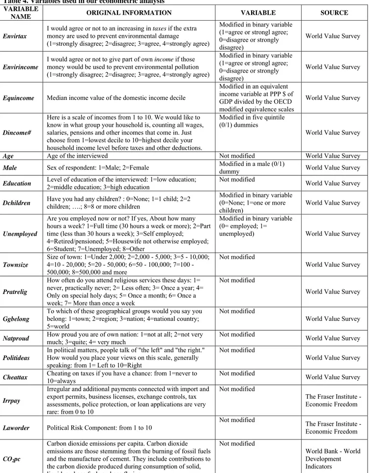
The set of additional controls includes three types of variables (individual sociodemographic, individual value and country variables). Individual sociodemographic variables include age, a gender dummy (male), a dummy for those who completed secondary education (education), a dummy measuring whether the interwieved has children (dchildren), an additional dummy introduced to pick up the effect of unemployment (unemployed) and, finally, the size of the town in which the respondent lives (townsize).
Among variables measuring individual’s values we include the intensity of religious practice (pratrelig), an indicator of care for global public goods (sense of belonging to a wider regional group) (ggbelong), a measure of national proudness (natproud), a variable measuring the inclination toward rightwing political ideas (politideas), an indicator of the individual opinion on tax evation (cheattax). Details on the construction of these variables are provided in Table 4.
The addition of these regressors is important as it helps us to net out the income effect from the concurring impact of proxies of personal values. In this way we can rule out the possibility that higher income individuals are more willing to pay for the environment just for the effect of these concurring factors associated with their higher income (i.e. different levels of social capital).
Among country variables we include proxies of domestic corruption (irrpay), of quality of institutions (laworder), a measure of domestic pollution (CO2pc) and of tax pressure (taxpress) (see
Table 4 for details). Year and country dummies are finally added to the specification.
4.1 Estimation approach
4 The World Value Survey database contains two variables which respectively provide the income
decile and the median household income value (in local currency) for that class for the majority of countries. For a second group of countries (Azerbaijan, Australia, Belarus, Israel, Armenia, Bangladesh, Belgium, Brazil, Colombia, Dominican Republic, Finland, Georgia, Hungary, Indonesia, Iran, Korea, Luxembourg, Nigeria, Pakistan, Philippines, Poland, Puerto Rico, Romania, Tanzania, United Kingdom, Viet Nam) sources of the missing median income value are the database of World Bank Development Indicators or, in alternative, Domestic Account data.
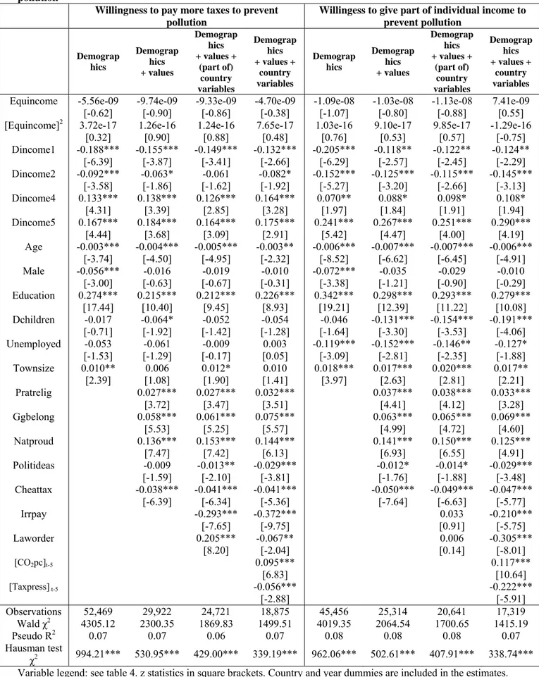
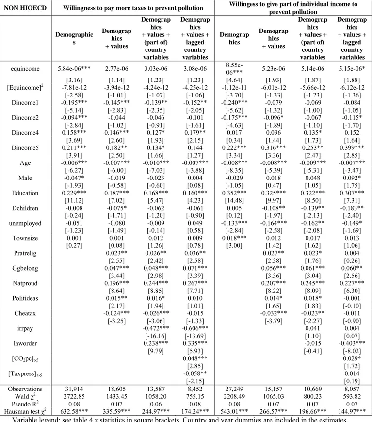
We estimate the model under four different specifications by considering alternatively as dependent variables the WTP more taxes and the willingness to provide additional income to prevent environmental pollution.5 In the first we just consider the impact of demographic variables (including relative and absolute income variables) and country dummies (Table 5, columns 1 and 5). In the second we introduce variables measuring individual values (concern for international public goods, tax morale, national proudness, political stance) (Table 5, columns 2 and 6). In the third, country variables related to corruption and quality of institutions (Table 5, columns 3 and 7). In the fourth two additional country variables (pollution intensity, measured in terms of per capita CO2, and overall tax pressure) which may be relevant control factors, but must be handled with care
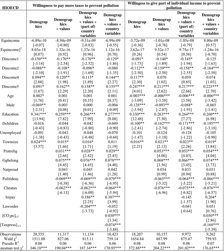
because of endogeneity (Table 5, columns 4 and 8). In Table 5 we estimate the model under the logit specification for the world sample by looking alternatively at the WTP more taxes and the willingness to provide additional income. In Tables 6 to 7 we propose robustness checks by estimating four different logit specifications for the subsamples of the high income OECD countries and the complenentary sample.6
4.1 Income
The most important finding in terms of income is that, while absolute income is not significant, relative income is significant and in the expected direction. The lack of significance of absolute income is likely to depend from the difficulties we have in measuring this variable (availability of only the income class median for each individual, conversion in dollars and in PPP). These problems, coupled with the presence of relative income and country dummy variables, probably eliminate any explanatory power of our absolute income proxy. When moving to relative income we find that the impact of income quintiles on both the tax and income equation is significantly negative (but increasing as far as we pass to higher income quintiles) below the median income and significantly positive above it. This result is reasonable since the omitted (third) quintile is the central one and therefore quintile dummies included in the estimate capture deviations from the effect of the omitted quintile on the dependent variable. Confidence intervals of the income quintile coefficients confirm that there is a significant change in the share of those willing to pay when we move from low to high income quintiles. To provide an example, the tax equation in the first column of Table 4 shows that coefficient magnitudes of the first and second quintiles are .19 and -.089 and both significantly different from zero at 99 percent level, while coefficient magnitudes of the fourth and fifth quintile dummies are .12 and .16, and significantly different from zero as well at the same significance level. Hence, individuals in the two highest quintiles exhibit significantly higher willingness to pay than those in the two lowest ones. The income equation also presents positive (negative) and significant coefficients for two upper (lower) quintiles.
This finding is remarkably stable across estimation methods (logit and ordered logit7) and subsample splits (high income OECD countries and the complementary sample) (Tables 6 and 7).8
5 Descriptive statistics and pairwise correlation matrix of variables used in the econometric estimates are provided in Appendix A.
6 The dependent variable takes the value of one if individuals strongly agree or agree (to pay more taxes or to give part of their income to prevent pollution) and the value of zero if they disagree or strongly disagree. In a robustness check we also reestimate the model for the world sample with an ordered logit specification. The dependent variable takes the value of three if individuals strongly agree, two if they agree and one if they disagree. It takes the value of zero otherwise. Estimates are omitted for reasons of space and available upon request.
7 Estimates are omitted for reasons of space and available upon request.
8 An additional robustness check on income effects, performed by running our specifications on country specific samples, confirms the presence of an income effect. Estimates are omitted and available upon request.
The hypothesis that the WTP for environmental protection becomes higher at higher income levels is not rejected by our findings even though, given the cross-sectional structure of the database, we cannot directly test whether an individual changes his WTP as far as his income grows.
4.2 Other demographics
Among the effects of other demografics we observe that younger and more educated individuals have higher willingness to pay for the environment. These findigs are also robust in all the reported subsample estimates (Tables 6 to 7) and consistent with those reported by Israely and Levinson (2001). The absence of repeated information for the same individuals is a problem for the age effect, as it is impossible to say whether we observe a temporal or a cohort effect. There are rationales in the literature to support both interpretations: younger generations may have grown with stronger environmental concerns, but also, as far as individuals get older, intertemporal discount rates may become higher in absence of intergenerational altruism.
An interesting finding is the negative and significant effect of the unemployment status on the willingness to give part of the income (Table 4, columns 5-8), but not on the willingness to pay additional taxes for the environment (Table 4, columns 1-4). The different impact on the two answers is reasonable if we assume that the willingness to pay has costs in the first, but presumably not in the second case (an unemployed should be tax exempt).
The positive and significant effect of town size in both equations is also understandable. Larger cities are expected to have relatively more severe environmental problems. What is interesting here is that individuals living in larger towns are also partially willing to internalize such externalities, as they probably clearly perceive their effects on the quality of their life and on their health.
An interesting finding is that a gender effect exists (women have significantly higher willingness to pay), but disappears once controlling for individual values. The most obvious interpretation is that the higher willingness to pay of women is explained by their relatively higher participation to the values (included in our estimates) which positively affect the propensity to pay to avoid pollution. Finally, the negative and significant effect of the presence of children in the respondent’s family in the income equation may be explained by the fact that this variable is likely to be a proxy of the household equivalised income.
4.3 Individual values
Some of the results on individual values are strongly stable across different specifications, estimation approaches and subsample splits. This is the case of the positive effect of religious practice (pratrelig), the sense of belonging to a wider regional group (ggbelong), national proudness (natproud) (all of them positive) and opinion about cheating on taxes (cheattax) (negative).
The positive and significant effect of religious practice is consistent with findings of Guiso et al. (2003) showing how religion reinforces civic values.
The sense of belonging to a wider regional group may be considered as a proxy of the respondent’s care (aversion) for global public goods (bads) and therefore its positive effect on the dependent variable (many environmental phenomena such as global heating and ozone layer depletion are global public bads) is reasonable. Another strongly significant variable in the estimate is tax morale. Individual blame on tax evasion is strongly positively correlated with the willingness to pay for the environment. Both national proudness and tax morale should be related to individual confidence in the use that domestic government could do of additional income to fight environmental degradation. Right wing political beliefs have negative and weakly significant effects on the dependent variable, probably showing that individuals with this political orientation put stronger confidence in the capacity of technological development of fighting environmental degradation, or are relatively less worried about the environmental problem. Our finding might also be affected by conditionality of
the interview bias to this variable (i.e. left wing oriented individuals may be more prone to give environmental friendly answers).
4.4 Country specific variables
Results on country specific variables are in some cases controversial (Tables 5,6 and 7, columns 3,4,7 and 8). The most stable and expected ones are the negative (positive) effect of domestic corruption (institutional quality) on the willigness to pay taxes. When moving to evaluate the effects of the other two country specific regressors (domestic pollution intensity and domestic tax pressure) we may have two different expectations according to whether individual preferences shape government behaviour (direct causality) or government behaviour affects individual preferences (reverse causality). With reference to pollution intensity, on the one side, we can think that individuals in their answers are conditioned by what the government already does and therefore their WTP is high if government commitment for the environment is low and pollution intensity high (positive relationship). On the other side, government preferences should reflect those of individuals and therefore, if the population has higher WTP for the environment, the equilibrium level of pollution intensity should be lower (negative relationship)
In a similar way, for tax pressure, the direct causality argument should imply that higher tax pressure has negative effect on the propensity to pay additional taxes against pollution, while the reverse causality argument should imply that higher tax morale should both determine higher tax pressure and willingness to pay for the environment. Given this potential reverse causality effect we introduce these last two variables only in the fourth specification in order to isolate their effects from the previously obtained findings (Tables 5, 6 and 7, columns 4 and 8) and lag of five years the two regressors.9 Our findings seem to support the direct causality argument in both cases. In short, individual willingness to pay taxes is higher the higher domestic pollution intensity and the lower the overall tax pressure.
4.5 Robustness check on regressors which vary at country level
A major problem in estimates on individuals belonging to different countries in which regressors include some variables varying at individual level and other varying at country level is that coefficients on the latter variables may be highly sensitive to inclusion or exclusion of a single country. In order to test whether it is the case we perform a two-step DFBETA test (for a similar approach see Frey and Stutzer, 2000). In the first step we estimate our fully augmented “tax model” with country dummies but without country variables. In the second step we create a dependent variable represented by coefficients of country dummies from the previous estimate and then regress it on the selected variables which vary at country level (i.e. , cheattax, irrpay, laworder, CO2pc, taxpress). 10 We then repeat this estimate by excluding any time one of the sample
countries. For each repeated estimate the coefficient is subtracted from the one obtained in the regression with all countries and divided by the estimated standard error. Table 8 finally reports the related F-test value. If the latter is lower than 1.96 in absolute value, the null of independence of our result from a country outlier is not rejected. Reported results clearly evidence that, in none of our four regressors varying at country level, we find an influential country outlier. 11
9 We also try to instrument the current values of these two variableswith lagged values, but the extremely low variability of these indicators across individuals (country effects are the same for all individuals of a given country) and across time prevents us to do so.
10 In this second step the number of observations is obviously equal to the number of countries in the sample.
11 Results on the income model (in which the dependent variable is the willingness to give part of income) also highlight that the null hypothesis is never rejected. They are omitted for reasons of space and available upon request.
4.6 Final comments
The use of a wide set of regressors shows that the relationship between income and WTP for the environment is independent from country specific culture and variables related to quality of institution, tax pressure, pollution intensity and corruption levels. It is also independent from a rich set of individual value indicators. Hence, whatever the country, the culture, the institutional environment and the set of individual values, richer individuals declare that they are more willing to pay for environmental quality. This higher willingness to pay, sufficient in demand side models (such as the one of Copeland and Taylor (2004) discussed in section 3) to generate an inverse U-shaped EKC, does not depend on the fact that higher income may be associated to different values, or to some cultures or countries, but is a pure income driven effect.
The significance of relative, and not absolute, income is important because it rules out the alternative rationale that the correlation between income and the WTP taxes is determined by the higher propensity to pay of richer countries (this last interpretation is also excluded by the fact that our result is robust when estimated in the subsample high income OECD estimate).
5. Conclusions
The link between empirical analyses and theoretical models may be of at least two types. More traditionally, statistical or econometric approaches tend to be used to test a specification derived from a theoretical construct. Alternatively, they may be used to test a crucial assumption on individual preferences which can generate a key result in a given, or in a class of, theoretical models.
We follow the second type of approach by considering that the inverse U-shaped relationship between per capita CO2 and per capita income, often observed in empirical papers in the
Environmental Kutznets Curve literature, may have demand and supply side explanations. A crucial element in the demand side explanation is the hypothesis that individuals have an elasticity of income to the marginal damage suffered from pollution which varies in the level of income. This assumption has seldom been directly tested.
In this paper we provide a straightforward test of it by controlling the effect of income on the willingness to pay for the environment for several (in some cases unexplored) concurring factors such as standard demographic variables, individual values, domestic corruption, institutional quality and level of pollution.
The richness of our controls helps to disentangle the income effect from other concurring effects. It tells us that the significantly higher willingness to pay for the environment for higher levels of income does not depend on differences in individual values and on domestic factors related to pollution intensity or confidence in domestic institutions.
References
Andreoni J., Levinson A., 1998. “The simple analytics of the Environmental Kuznets Curve”, NBER Working Paper 6739.
Antweiler, W., Copeland, B. R., e Taylor, M. S., 2001. “Is free trade good for the environment?”, American Economic Review, 91: 877-908.
Bird, K. & Hughes, D.: 1997, ‘Ethical consumerism: the case of “fairly-traded” coffee, Business
Ethics: a European Review, 6, 3, pp.159-167
Borghesi S., 2000. “Income inequality and the Environmental Kuznets Curve”, Nota di Lavoro FEEM 83/2000.
Borghesi, S., 2001. “The environment Kuznets curve: a critical survey”, Fondazione ENI Enrico Mattei, Working Paper 85ּ99.
Borghesi, S., 2005. “The Kuznets curve and the environmental Kuznets curve:A simple steady-state analysis”, Rivista Internazionale di Studi Economici e Commerciali, Università Bocconi-CEDAM, Padova, (52): 35-61. Carson, Richard T.; Robert Cameron Mitchell. 1995. “Sequencing and Nesting in Contingent Valuation Surveys.” Journal of Environmental Economics and Management, Volume: 28, Issue: 2, Pages: 155-173.
Cole, M. A., Rayner, A. J. e Bates, J. M., 1997. “The environmental Kuznets curve: an empirical analysis”, Environment and Development Economics, 2: 401-416.
Cole, M. A., Elliott, R. J., 2003. “Determining the trade–environment composition effect: The role of capital,
labour and environmental regulations”, Journal of Environmental Economics and Management, (46): 363–
383.
Common, M., 1995. “Sustainable and Policy”, Cambridge University Press, Cambridge.
Copeland, B. R. e Taylor M., 2004. “Trade, Growth, and the Environment”, Journal of Economic Literature, 42 (1): 7-71.
Dasgupta, S., Laplante, B., Wang, H., e Wheeler, D., 2002. “Confronting the environmental Kuznets curve”, Journal of Economic Perspectives, 16: 147-168.
De Benedictis, L. e Helg, R., 2002. “Globalizzazione”, Rivista di Politica Economica, marzo-aprile, 92 (3-4): 139-209.
Demos & Pi / Coop, 2004, Osservatorio sul Capitale sociale Virtù e valori degli italiani, Indagine 2004
De Pelsmacker, P. Driesen L. Rayp G., 2003, Are fair trade labels good business ? ethics and coffee buying intentions. Workign paper University of Gent.
Grossman, G. e Krueger A., 1991. “Environmental impacts of a North American Free Trade Agreement”, National Bureau of Economic Research Working Paper 3914, NBER, Cambridge MA.
B. S. Frey and A. Stutzer, Happiness, Economy and Institutions, The Economic Journal, 110 (466, October), 2000, pp. 918-938
Grossman, G. e Krueger A., 1993. “Environmental Impacts of a North American Free Trade Agreement,”, The U.S.-Mexico Free Trade Agreement. Peter M. Garber, ed. Cambridge, MA: MIT Press, pp. 13–56.
Grossman, G. e Krueger, A., 1994. “Economic growth and the environment”, NBER, Working Paper 4634, Febbraio.
Guiso, L., Sapienza, P. & Zingales, L. (2003), 'People's opium ? Religion and economic attitudes', Journal of Monetary Economics 50, 225 282.
Islam, N., Vincent, J., e Panayotou, T., 1999. “Unveiling the Income-Environment Relationship: an
Exploration into the Determinants of Environmental Quality”, Department of Economics and Harvard Institute
for International Development, Working Paper 701.
Israel, D., e Levinson, A., 2002. “Willingness to Pay for Environmental Quality: Testable Empirical
Implications of the Growth and Environment Literature”, Contributions to Economic Analysis & Policy, 1 (1):
art 3.
Israel, D., e Levinson, A., 2004. “Willingness to Pay for Environmental Quality: Testable Empirical
Implications of the Growth and Environment Literature”, Contributions to Economic Analysis & Policy, 3 (1):
art 2.
IPCC, 1992. “Intergovernmental Institute for Applied Systems Analysis”, Science and sustainability, Novographic, Vienna.
Jaffe, A. B., Peterson, S. R., Portney, P. R., e Stavins, R. N., 1995. “Environmental regulation and the
competitiveness of US manufacturing: What does the evidence tell us?”, Journal of Economic Literature, 33:
132–163.
Kahneman, D.; Knetsch, J. (1992) Valuing Public Goods: The Purchase of Moral Satisfaction, Journal of Environmental Economics and Management 22, 57-70.
Kuznets, S., 1955. “Economic growth and income inequality”, American Economic Review, 45 (1): 1-28. Lopez, R., 1994. “The environment as a factor of production: the effects of economic growth and trade
liberalization”, Journal of Environmental Economics and Management, 27: 163-184.
Lopez, R. e Mitra S., 2000. “Corruption, Pollution and the Environmental Kuznets Curve”, Journal of Environmental Economics Manage, 40 (2): 137–50.
Lucas, R. E. B., Wheeler, D., e Hettige, H., 1992. “Economic development, environmental regulation and the
international migration of toxic industrial pollution: 1960-1988”, P. Low (Editor), International Trade and the
Environment, World Bank Discussion Paper No. 159, Washington DC.
Magnani E., 2000. “The Environmental Kuznets Curve, environmental protection policy and income
distribution”, Ecological Economics, 32: 431-443.
Moore, G., 2004, The Fair Trade Movement: parameters, issues and future research, Journal of Business Ethics, 53, 73-86
Panayotou, T., 1993. “Empirical Tests and Policy Analysis of Environmental Degradation at Different Stages
of Economic Development”, Technology and Employment Programme, International Labour Office, Geneva,
Working Paper WP238.
Panayotou, T., 1997. “Demystifying the environmental Kuznets curve: turning a black box into a policy tool”, Environment and Development Economics, 2: 465-484.
Panayotou, T., Peterson A., e Sachs J., 2000. “Is the Environmental Kuznets Curve Driver by Structural
Change?”, mimeo, Center Int. Develop., Harvard U.
Panayotou, T., 2000. “Economic Growth and the Environment”, Environment and Development, CID Working Paper 56 (4).
Perman, R. e Stern, D. I., 2003. “Evidence from panel unit root and cointegration tests that the environmental
Kuznets curve does not exist”, Australian Journal of Agricultural and Resource Economics, Vol. 47.
Randall, A. and Hoehn, JP, 1996, Embedding in market demand systems, Journal of Environmental Economics and Management, 30: 369-380.
Selden, T. M. e Song D., 1994. “Environmental quality and development: Is there a Kuznets curve for air
pollution?”, Journal of Environmental Economics and Environmental Management, 27: 147-162.
Selden, T. M. e Song, D., 1995. “Neoclassical growth, the J curve for abatement and the inverted U curve for
pollution”, Journal of Environmental Economics and Environmental Management, 29: 162-168.
Selden, T. M., Forrest, A. S., e Lockhart, J. E., 1999. “Analyzing reductions in U.S. air pollution emissions:
1970 to 1990”, Land Economics, 75:1-21.
Shafik, N., 1994. “Economic development and environmental quality: an econometric analysis”, Oxford Economic Papers, 46: 757-773.
Shafik, N. e Bandyopadhyay, S., 1992. “Economic Growth and Environmental Quality: Time Series and
Cross-Country Evidence”, Background Paper for the World Development Report 1992, World Bank,
Washington DC.
Solow, R.M., 1986. “On the intergenerational allocation of natural resources”, Scand. Journal Economics, 88: 141–149.
Stern, D. I., Common, M. S., e Barbier, E. B., 1996. “Economic growth and environmental degradation: The
environmental Kuznets curve and sustainable development”, World Development, (24): 1151–1160.
Stern, D. I. e Common, M. S., 2001. “Is there an environmental Kuznets curve for sulfur?”, Journal of Environmental Economics and Environmental Management, 41: 162 178.
Stern, D., 2003. “The Environmental Kuznets Curve”, International Society for Ecological Economics, Internet Encyclopaedia of Ecological Economics, Department of Economics, Rensselaer Polytechnic Institute, Troy, NY 12180, USA.
Stern, D., 2004. “The Rise and Fall of the Environmental Kuznets Curve”, World Development, 32 (8): 1419-39.
Stiglitz, J. E., 2002. “La Globalizzazione e i suoi oppositori”, Enaudi editore, Torino.
Stokey, N. L., 1998. “Are there limits to growth?”, International Economic Review, 39 (1): 1–31.
Suri, V. e Chapman, D., 1998. “Economic growth, trade and the energy: implications for the environmental
Torgler, B., e Garcia-Valinas, M. A., 2005. “The Willingness to Pay for preveting Environmental Damage”, Working Paper 22, Center for Reserch in Economics, Management and the Arts.
Table 1. Willingness to pay for the environment: descriptive evidence at world level
I would agree to an increase in taxes if the extra money were used to prevent environmental damage (in WVSs 1990–1993 and 1995-1997), I would agree to an increase in taxes if the extra money were used to prevent environmental pollution (in WVS 2001)
Strongly
disagree Disagree Agree Strongly agree N. of obs
World 7,130 17,399 33,504 12,295 70,328
(10.14%) (24.74%) (47.64%) (17.48%) (100%)
High income OECD
countries 3,486 6,968 12,053 3,544 26,051
(13.38%) (26.75%) (46.27%) (13.60%) (37.04%)
Non high income OECD
countries 3,644 10,431 21,451 8,751 44,277
(8.23%) (23.56%) (48.45%) (19.76%) (62.96%)
I would give part of my income if I were certain that the money would be used to prevent environmental pollution (in WVS 2001)
Strongly
disagree Disagree Agree Strongly agree N. of obs World 21,303 55,831 83,377 30,699 191,210
(11.14%) (29.20%) (43.60%) (16.06%) (100%)
High income OECD
countries 9,497 21,367 31,688 9,622 72,174
(13.16%) (29.60%) (43.91%) (13.33%) (37.74%)
Non high income OECD
countries 11,806 34,464 51,689 21,077 119,036
(38.87%) (28.95%) (43.42%) (17.71%) (62.26%) High income OECD countries: Australia, Austria, Belgium, Canada, Denmark, Finland, France, Germany, Greece, Iceland, Ireland,
Italy, Japan, Luxembourg, Netherlands, New Zealand, Norway, Portugal, Spain, Sweden, Switzerland, United Kingdom, United States of America.
Non high income OECD countries: Albania, Algeria, Azerbaijan, Argentina, Armenia, Bangladesh, Bosnia Herzegovina, Brazil,
Bulgaria, Belarus, Chile, China, Taiwan, Colombia, Croatia, Czech Republic, Dominican Republic, Egypt, El Salvador, Estonia, Georgia, Hungary, India, Indonesia, Iran, Israel, Jordan, Korea, Latvia, Lithuania, Macedonia, Malta, Mexico, Moldova, Montenegro, Morocco, Nigeria, North Ireland, Pakistan, Peru, Philippines, Poland, Puerto Rico, Romania, Russian Federation, Serbia, Singapore, Slovakia, Slovenia, South Africa, Tanzania, Turkey, Zimbabwe, Uganda, Ukraine, Uruguay, Venezuela, Viet Nam, Zimbabwe.
Table 2.A Willingness to pay for the environment: country rankings
I would agree to an increase in taxes if the extra money were used to prevent environmental damage (in WVSs 1990–1993 and 1995-1997), I would agree to an increase in taxes if the extra money were used to prevent environmental pollution (in WVS 2001). Country Strongly disagree or disagree Agree or strongly agree N. of obs. VIETNAM 89 9.55% 843 90.45% 932 DOMINICAN REPUBLIC 56 13.76% 351 86.24% 407 EL SALVADOR 193 16.00% 1,013 84.00% 1206 BANGLADESH 478 17.57% 2,243 82.43% 2721 CHINA 737 18.57% 3,231 81.43% 3968 GHANA 19 20.88% 72 79.12% 91 SWEDEN 627 20.90% 2,373 79.10% 3000 PUERTO RICO 406 22.01% 1,439 77.99% 1845 TANZANIA 290 25.44% 850 74.56% 1140 NORWAY 600 25.73% 1,732 74.27% 2332 BRAZIL 812 28.12% 2,076 71.88% 2888 TURKEY 1,161 29.09% 2,830 70.91% 3991 KOREA 1,074 30.09% 2,495 69.91% 3569
SERBIA AND MONTENEGRO 1,035 30.27% 2,384 69.73% 3419
GEORGIA 600 31.12% 1,328 68.88% 1928
AUSTRALIA 630 31.30% 1,383 68.70% 2013
BOSNIA AND HERZEGOVINA 735 31.96% 1,565 68.04% 2300
CHILE 1,173 32.43% 2,444 67.57% 3617 CZECH REPUBLIC 895 32.47% 1,861 67.53% 2756 COLOMBIA 970 32.61% 2,005 67.39% 2975 DENMARK 650 32.68% 1,339 67.32% 1989 SLOVENIA 979 34.31% 1,874 65.69% 2853 GREECE 390 35.20% 718 64.80% 1108 VENEZUELA,RB 409 35.53% 742 64.47% 1151 MACEDONIA,FYR 692 36.54% 1,202 63.46% 1894 SPAIN 4,741 37.05% 8,056 62.95% 12797 CROATIA 784 37.28% 1,319 62.72% 2103 ALBANIA 341 37.39% 571 62.61% 912 RUSSIAN FEDERATION 2,774 37.81% 4,563 62.19% 7337 NETHERLANDS 763 38.17% 1,236 61.83% 1999 BELARUS 1,457 38.28% 2,349 61.72% 3806 CANADA 1,392 38.68% 2,207 61.32% 3599 NIGERIA 1,443 39.30% 2,229 60.70% 3672 JAPAN 1,147 39.66% 1,745 60.34% 2892 UNITED STATES 1,773 39.82% 2,680 60.18% 4453 PHILIPPINES 948 39.98% 1,423 60.02% 2371 BULGARIA 1,116 40.13% 1,665 59.87% 2781 MEXICO 1,750 40.31% 2,591 59.69% 4341 URUGUAY 392 40.37% 579 59.63% 971 PERU 1,060 40.61% 1,550 59.39% 2610 INDIA 2,228 40.74% 3,241 59.26% 5469 ICELAND 682 41.59% 958 58.41% 1640 ARMENIA 821 43.07% 1,085 56.93% 1906
Table 2.A (follows) Willingness to pay for the environment: country rankings*
I would agree to an increase in taxes if the extra money were used to prevent environmental damage (in WVS 1990–1993 e 1995 1997), I would agree to an increase in taxes if the extra money were used to prevent environmental pollution (in WVS 2001).
Country Strongly disagree or disagree Agree or strongly agree N. of obs. UNITED KINGDOM 1,533 43.33% 2,005 56.67% 3,538 PORTUGAL 886 43.88% 1,133 56.12% 2,019 LUXEMBOURG 517 44.96% 633 55.04% 1,150 AZERBAIJAN 842 45.12% 1,024 54.88% 1,866 NEW ZEALAND 488 45.14% 593 54.86% 1,081 LATRIA 1,295 45.71% 1,538 54.29% 2,833 UCRAINE 1,514 45.98% 1,779 54.02% 3,293 FINLAND 1,175 46.37% 1,359 53.63% 2,534 MOLDOVA 830 46.42% 958 53.58% 1,788 POLAND 995 47.65% 1,093 52.35% 2,088 ESTONIA 1,413 49.23% 1,457 50.77% 2,870 GERMANY 3,579 50.03% 3,575 49.97% 7,154 ITALY 1,964 50.53% 1,923 49.47% 3,887 MALTA 515 52.13% 473 47.87% 988 LITHUANIA 1,465 53.53% 1,272 46.47% 2,737 ROMANIA 518 53.57% 449 46.43% 967 ZIMBABWE 500 53.82% 429 46.18% 929 ARGENTINA 1,754 54.34% 1,474 45.66% 3,228 IRELAND 1,068 54.66% 886 45.34% 1,954 SINGAPORE 816 54.95% 669 45.05% 1,485 AUSTRIA 1,553 55.21% 1,260 44.79% 2,813 SLOVAK REPUBLIC 963 55.47% 773 44.53% 1,736 UGANDA 556 56.05% 436 43.95% 992 FRANCE 1,425 56.30% 1,106 43.70% 2,531 SWITZERLAND 660 56.99% 498 43.01% 1,158 BELGIUM 2,621 57.82% 1,912 42.18% 4,533 SOUTH AFRICA 3,111 57.83% 2,269 42.17% 5,380 HUNGARY 1,266 65.73% 660 34.27% 1,926 77,134 40.34% 114,076 59.66% 191,210 Number of observations
Table 2.B Willingness to pay for the environment: country rankings
I would give part of my income if I were certain that the money would be used to prevent environmental pollution (in WVS 2001)
Country Strongly disagree or disagree Agree or strongly agree N. of obs. VIETNAM 38 3.98% 917 96.02% 955 TANZANIA 177 15.62% 956 84.38% 1,133 REPUBLIC OF KOREA 167 16.32% 856 83.68% 1,023 CROATIA 171 17.59% 801 82.41% 972 GREECE 198 17.82% 913 82.18% 1,111 SLOVENIA 174 17.96% 795 82.04% 969 PUERTO RICO 128 18.00% 583 82.00% 711 CHINA 161 18.01% 733 81.99% 894 PERU 275 19.10% 1,165 80.90% 1,440 BANGLADESH 281 20.50% 1,090 79.50% 1,371 MEXICO 301 20.90% 1,139 79.10% 1,440 MACEDONIA 210 21.06% 787 78.94% 997 DENMARK 207 21.14% 772 78.86% 979 SWEDEN 213 21.19% 792 78.81% 1,005 CZECH REPUBLIC 417 22.79% 1,413 77.21% 1,830 TURKEY 272 23.49% 886 76.51% 1,158 BOSNIA-HERZEGOVINA 282 24.33% 877 75.67% 1,159 NETHERLANDS 257 25.73% 742 74.27% 999 PHILIPPINES 325 27.61% 852 72.39% 1,177 SERBIA 590 28.88% 1,453 71.12% 2,043 LATVIA 278 29.54% 663 70.46% 941 CHILE 346 29.65% 821 70.35% 1,167 JAPAN 326 29.80% 768 70.20% 1,094 ALBANIA 272 29.89% 638 70.11% 910 CANADA 575 30.34% 1,320 69.66% 1,895 USA 365 30.70% 824 69.30% 1,189 ZIMBABWE 290 30.82% 651 69.18% 941 MOLDOVA 284 31.66% 613 68.34% 897 INDIA 487 32.97% 990 67.03% 1,477
Table 2.B (follows) Willingness to pay for the environment: country rankings
I would give part of my income if I were certain that the money would be used to prevent environmental pollution (in WVS 2001)
Country Strongly disagree or disagree Agree or strongly agree N. of obs. ARGENTINA 407 33.22% 818 66.78% 1,225 ITALY 666 35.20% 1,226 64.80% 1,892 LUXEMBOURG 414 36.28% 727 63.72% 1,141 ICELAND 347 36.53% 603 63.47% 950 SINGAPORE 548 36.83% 940 63.17% 1,488 UKRAINE 403 36.90% 689 63.10% 1,092 RUSSIA 848 37.36% 1,422 62.64% 2,270 BULGARIA 362 38.97% 567 61.03% 929 POLAND 404 39.19% 627 60.81% 1,031 MALTA 392 39.72% 595 60.28% 987 PORTUGAL 375 40.41% 553 59.59% 928 BELGIUM 750 40.45% 1,104 59.55% 1,854 SPAIN 941 41.53% 1,325 58.47% 2,266 BELARUS 390 42.30% 532 57.70% 922 SLOVAKIA 552 43.29% 723 56.71% 1,275 IRELAND 435 45.17% 528 54.83% 963 FINLAND 460 46.28% 534 53.72% 994 HUNGARY 452 46.45% 521 53.55% 973 SOUTH AFRICA 1,289 47.32% 1,435 52.68% 2,724 ROMANIA 465 47.79% 508 52.21% 973 AUSTRIA 754 51.36% 714 48.64% 1,468 ESTONIA 477 51.90% 442 48.10% 919 UNITED KINGDOM 959 53.25% 842 46.75% 1,801 FRANCE 851 54.17% 720 45.83% 1,571 UGANDA 531 55.03% 434 44.97% 965 GERMANY 1,361 69.76% 590 30.24% 1,951 LITHUANIA 629 69.97% 270 30.03% 899 Number of observations 24,529 34.88% 45,799 65.12% 70,328
Table 3.A Willingness to pay for the environment and income quintiles
I would agree to an increase in taxes if the extra money were used to prevent environmental damage (in WVSs 1990–1993 and 1995-1997), I would agree to an increase in taxes if the extra money were used to prevent environmental pollution (in WVS 2001). (Total number of observations 163,620)
Income ranges Disagree Strongly
disagree Agree
Strongly
agree N. of obs. Cumulative distr. 1st quintile 4,690 11,051 14,818 6,061 36,620 12.81% 30.18% 40.46% 16.55% 22.38% 22.38% 2nd quintile 5,346 14,446 20,917 7,471 48,180 11.10% 29.98% 43.41% 15.51% 29.45% 51.83% 3rd quintile 3,714 10,933 17,851 6,205 38,703 9.60% 28.25% 46.12% 16.03% 23.65% 75.48% 4th quintile 2,178 6,561 11,306 4,282 24,327 8.95% 26.97% 46.48% 17.60% 14.87% 90.35% 5th quintile 1,688 4,148 7,136 2,818 15,790 10.69% 26.27% 45.19% 17.85% 9.65% 100.00%
Table 3.B Willingness to pay for the environment and income quintiles
I would give part of my income if I were certain that the money would be used to prevent environmental pollution (in WVS 2001) (Total number of observations 61,067)
Income ranges Disagree Strongly
disagree Agree
Strongly
agree N. of obs. Cumulative distr. 1st quintile 1,687 3,427 5,757 2,352 13,223 12.76% 25.92% 43.54% 17.79% 21.65% 21.65% 2nd quintile 1,969 4,608 8,168 3,003 17,748 11.09% 25.96% 46.02% 16.92% 29.06% 50.72% 3rd quintile 1,203 3,465 7,587 2,754 15,009 8.02% 23.09% 50.55% 18.35% 24.58% 75.29% 4th quintile 673 2,135 4,892 1,793 9,493 7.09% 22.49% 51.53% 18.89% 15.55% 90.84% 5th quintile 362 1,106 2,939 1,187 5,594 6.47% 19.77% 52.54% 21.22% 9.16% 100.00%
Table 4. Variables used in our econometric analysis
VARIABLE
NAME ORIGINAL INFORMATION VARIABLE SOURCE
Envirtax
I would agree or not to an increasing in taxes if the extra money are used to prevent environmental damage
(1=strongly disagree; 2=disagree; 3=agree, 4=strongly agree)
Modified in binary variable (1=agree or strongl agree; 0=disagree or strongly disagree)
World Value Survey
Envirincome
I would agree or not to give part of own income if those money would be used to prevent environmental pollution (1=strongly disagree; 2=disagree; 3=agree, 4=strongly agree)
Modified in binary variable (1=agree or strongl agree; 0=disagree or strongly disagree)
World Value Survey
Equincome Median income value of the domestic income decile
Modified in an equivalent income variable at PPP $ of GDP divided by the OECD modified equivalence scales
World Value Survey
Dincome#
Here is a scale of incomes from 1 to 10. We would like to know in what group your household is, counting all wages, salaries, pensions and other incomes that come in. Just choose from 1=lowest decile to 10=highest decile your household income level before taxes and other deductions.
Modified in five quintile (0/1) dummies
World Value Survey
Age Age of the interviewed Not modified World Value Survey
Male Sex of respondent: 1=Male; 2=Female Modified in a male (0/1) dummy World Value Survey Education Level of education of the interviewed: 1=low education; 2=middle education; 3=high education Not modified World Value Survey
Dchildren Have you had any children? : 0=None; 1=1 child; 2=2 children; ….; 8=8 or more children
Modified in binary variable (0=None; 1=one or more
children) World Value Survey
Unemployed
Are you employed now or not? If yes, About how many hours a week? 1=Full time (30 hours a week or more); 2=Part time (less than 30 hours a week); 3=Self employed;
4=Retired/pensioned; 5=Housewife not otherwise employed; 6=Student; 7=Unemployed; 8=Other
Modified in binary variable (0= employed; 1=
unemployed) World Value Survey
Townsize
Size of town: 1=Under 2,000; 2=2,000 - 5,000; 3=5 - 10,000; 4=10 - 20,000; 5=20 - 50,000; 6=50 - 100,000; 7=100 - 500,000; 8=500,000 and more
Not modified
World Value Survey
Pratrelig
How often do you attend religious services these days: 1= never, practically never; 2= Less often; 3= Once a year; 4= Only on special holy days; 5= Once a month; 6= Once a week; 7= More than once a week
Not modified
World Value Survey
Ggbelong
To which of these geographical groups would you say you belong: 1=town; 2=region; 3=nation; 4=national country; 5=world
Not modified
World Value Survey
Natproud How proud you are of own nation: 1=not at all; 2=not very much; 3=quite; 4= very much Not modified World Value Survey
Politideas
In political matters, people talk of "the left" and "the right." How would you place your views on this scale, generally speaking: from 1= Left to 10=Right
Not modified
World Value Survey
Cheattax Cheating on taxes if you have a chance: from 1=never to 10=always Not modified World Value Survey
Irrpay
Irregular and additional payments connected with import and export permits, business licenses, exchange controls, tax assessments, police protection, or loan applications are very rare: from 0 to 10
Not modified
The Fraser Institute - Economic Freedom
Laworder Political Risk Component: from 1 to 10
Not modified The Fraser Institute - Economic Freedom
CO2pc
Carbon dioxide emissions per capita. Carbon dioxide emissions are those stemming from the burning of fossil fuels and the manufacture of cement. They include contributions to the carbon dioxide produced during consumption of solid, liquid, and gas fuels and gas flaring
Not modified
World Bank - World Development Indicators
Taxpress
Top marginal income and payroll tax rates (and income thresholds at which they apply). Countries with higher marginal tax rates that take effect at lower income thresholds received lower ratings: from 1 to 10
Not modified
The Fraser Institute - Economic Freedom
Table 5. The determinants of the willingness to pay more taxes or to give part of individual income to prevent pollution
Willingness to pay more taxes to prevent pollution
Willingess to give part of individual income to prevent pollution Demograp hics Demograp hics + values Demograp hics + values + (part of) country variables Demograp hics + values + country variables Demograp hics Demograp hics + values Demograp hics + values + (part of) country variables Demograp hics + values + country variables Equincome -5.56e-09 -9.74e-09 -9.33e-09 -4.70e-09 -1.09e-08 -1.03e-08 -1.13e-08 7.41e-09
[-0.62] [-0.90] [-0.86] [-0.38] [-1.07] [-0.80] [-0.88] [0.55] [Equincome]2 3.72e-17 1.26e-16 1.24e-16 7.65e-17 1.03e-16 9.10e-17 9.85e-17 -1.29e-16 [0.32] [0.90] [0.88] [0.48] [0.76] [0.53] [0.57] [-0.75] Dincome1 -0.188*** -0.155*** -0.149*** -0.132*** -0.205*** -0.118** -0.122** -0.124** [-6.39] [-3.87] [-3.41] [-2.66] [-6.29] [-2.57] [-2.45] [-2.29] Dincome2 -0.092*** -0.063* -0.061 -0.082* -0.152*** -0.125*** -0.115*** -0.145*** [-3.58] [-1.86] [-1.62] [-1.92] [-5.27] [-3.20] [-2.66] [-3.13] Dincome4 0.133*** 0.138*** 0.126*** 0.164*** 0.070** 0.088* 0.098* 0.108* [4.31] [3.39] [2.85] [3.28] [1.97] [1.84] [1.91] [1.94] Dincome5 0.167*** 0.184*** 0.164*** 0.175*** 0.241*** 0.267*** 0.251*** 0.290*** [4.44] [3.68] [3.09] [2.91] [5.42] [4.47] [4.00] [4.19] Age -0.003*** -0.004*** -0.005*** -0.003** -0.006*** -0.007*** -0.007*** -0.006*** [-3.74] [-4.50] [-4.95] [-2.32] [-8.52] [-6.62] [-6.45] [-4.91] Male -0.056*** -0.016 -0.019 -0.010 -0.072*** -0.035 -0.029 -0.010 [-3.00] [-0.63] [-0.67] [-0.31] [-3.38] [-1.21] [-0.90] [-0.29] Education 0.274*** 0.215*** 0.212*** 0.226*** 0.342*** 0.298*** 0.293*** 0.279*** [17.44] [10.40] [9.45] [8.93] [19.21] [12.39] [11.22] [10.08] Dchildren -0.017 -0.064* -0.052 -0.054 -0.046 -0.131*** -0.154*** -0.191*** [-0.71] [-1.92] [-1.42] [-1.28] [-1.64] [-3.30] [-3.53] [-4.06] Unemployed -0.053 -0.061 -0.009 0.003 -0.119*** -0.152*** -0.146** -0.127* [-1.53] [-1.29] [-0.17] [0.05] [-3.09] [-2.81] [-2.35] [-1.88] Townsize 0.010** 0.006 0.012* 0.010 0.018*** 0.017*** 0.020*** 0.017** [2.39] [1.08] [1.90] [1.41] [3.97] [2.63] [2.81] [2.21] Pratrelig 0.027*** 0.027*** 0.032*** 0.037*** 0.038*** 0.033*** [3.72] [3.47] [3.51] [4.41] [4.12] [3.28] Ggbelong 0.058*** 0.061*** 0.075*** 0.063*** 0.065*** 0.069*** [5.53] [5.25] [5.57] [4.99] [4.72] [4.60] Natproud 0.136*** 0.153*** 0.144*** 0.141*** 0.150*** 0.125*** [7.47] [7.42] [6.13] [6.93] [6.55] [4.91] Politideas -0.009 -0.013** -0.029*** -0.012* -0.014* -0.029*** [-1.59] [-2.10] [-3.81] [-1.76] [-1.88] [-3.48] Cheattax -0.038*** -0.041*** -0.041*** -0.050*** -0.049*** -0.047*** [-6.39] [-6.34] [-5.36] [-7.64] [-6.63] [-5.77] Irrpay -0.293*** -0.372*** 0.033 -0.210*** [-7.65] [-9.75] [0.91] [-5.75] Laworder 0.205*** -0.067** 0.006 -0.305*** [8.20] [-2.04] [0.14] [-8.01] [CO2pc]t-5 0.095*** 0.117*** [6.83] [10.64] [Taxpress] t-5 -0.056*** -0.222*** [-2.88] [-5.91] Observations 52,469 29,922 24,721 18,875 45,456 25,314 20,641 17,319 Wald χ2 4305.12 2300.35 1869.83 1499.51 4019.35 2064.54 1700.65 1415.19 Pseudo R2 0.07 0.07 0.06 0.07 0.08 0.08 0.08 0.07 Hausman test χ2 994.21*** 530.95*** 429.00*** 339.19*** 962.06*** 502.61*** 407.91*** 338.74*** Variable legend: see table 4. z statistics in square brackets. Country and year dummies are included in the estimates.