DOTTORATO DI RICERCA IN
Ingegneria Ambientale, Civile e dei Materiali
Ciclo XXVIII
Settore Concorsuale di afferenza: 08 A2
Settore Scientifico disciplinare: ING/IND 30
TITOLO TESI
Numerical modelling and simulation optimization of geothermal
reservoirs using the TOUGH2 family of codes
Presentata da: Ester Maria Vasini
Coordinatore Dottorato
Relatore
Prof. Alberto Lamberti Prof. Villiam Bortolotti
Correlatore
Ing. Alfredo Battistelli
In order to improve the reservoir engineering activities and, in particular, to optimize numerical modelling and simulation of geothermal reservoirs using the TOUGH family of codes, it has been decided to use the software T2Well for the interpretation of well-tests, coupling T2Well with the equation of state module EWASG, which describes the typical thermodynamic condition in high enthalpy geothermal reservoirs. T2Well-EWASG has been coupled and tested through the typical process of verification and validation. The application of T2Well-EWASG for the interpretation of well-tests related to the slim hole WW-01 drilled in the Wotten Waven Field (Commonwealth of Dominica) proves that it can be used as a tool for integrated interpretation of surface and downhole measurements collected during the performance of production tests in geothermal wells. The strength of this tool is that it allows to reduce the different possible solutions (in terms of reservoir characterization) within an acceptable error, by allowing the interpretation of surface and downhole measurements in conjunction, instead of separately. From this point of view T2Well-EWASG can effectively be used as a tool which allows an improvement of reservoir engineering activities. Finally, the huge amount of data managed during these activities has permitted to test and project the improvement of pre- and post- processing tools specific for TOUGH2 created by the geothermal research group of DICAM. In particular, the pre- and post-processing tools have been validated with a case study dealing with the migration of non-condensable gases in deep sedimentary formation.
Contents
NOMENCLATURE ... I
INTRODUCTION ... 5
1 BACKGROUND ... 9
1.1 SYSTEM, MODEL, CALIBRATION AND SIMULATION ... 9
1.2 NUMERICAL RESERVOIR SIMULATION ... 10
1.2.2 Reservoir Simulators ... 14
1.2.2.1 Brief overview on TOUGH family of codes ... 15
1.2.2.2 Pre- and Post-processing tools for TOUGH family of codes ... 17
1.2.3 Coupled Wellbore-Reservoir Simulators... 17
2 TOUGH2, T2WELL, TOUGH2VIEWER AND VORO2MESH ... 23
2.1TOUGH2... 23
2.1.1 Mass and energy balance ... 25
2.1.2 Space and time discretization ... 26
2.1.3 Brief input file description ... 28
2.1.4 EWASG EOS MODULE ... 29
2.1.4.1 Thermodynamic description ... 30
2.2T2WELL ... 35
2.2.1 Mass and energy balance ... 35
2.2.2 Drift Flux Model ... 37
2.2.3 Discretized equations ... 40
2.2.4 Heat exchange ... 40
2.3VORO2MESH AND TOUGH2VIEWER ... 41
2.3.1 Grid type ... 42
2.3.2 Voronoi diagrams ... 43
2.3.3 VORO2MESH ... 44
2.3.4 TOUGH2Viewer ... 45
3.1ANALYTICAL COMPUTATION OF HEAT EXCHANGE ... 47
3.2T2WELL SOURCE CODE ... 52
3.3T2WELL INPUT FILE ... 53
4 MODEL VERIFICATION &VALIDATION ... 57
4.1VERIFICATION AND VALIDATION ... 57
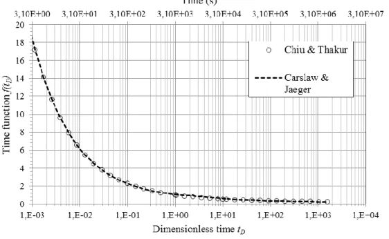
4.2VERIFICATION OF ANALYTICAL HEAT EXCHANGE ... 58
4.3VALIDATION ... 61
4.3.1 Reproduction of flowing pressure and temperature profiles ... 61
4.3.2 Application of T2Well for the interpretation of well-tests ... 66
5 APPLICATION OF TOUGH2VIEWER AND VORO2MESH ... 77
5.1TMGASEOSMODULE ... 78
5.2MODEL AND GRIDS DESCRIPTION ... 79
5.3SIMULATION RESULTS ... 82
6 CONCLUSIONS ... 87
6.1TOUGH2VIEWER AND VORO2MESH APPLICATION... 87
6.2T2WELL-EWASG ... 87
6.3FUTURE WORK ... 89
6.3.1 Inverse simulation ... 89
6.3.2 Analytical computation of heat exchange ... 89
6.3.3Non-Darcy flow near the wellbore ... 90
Nomenclature
A Cross sectional area m2
b0, b1, b2 Constant coefficients
b3, b4 Polynomial function of the temperature
C Specific heat J°C-1kg-1
C0 Profile parameter
d Wellbore diameter m
D, D1 Salt concentration polynomials
E0, E1, E2, E3, E4 Pressure dependent coefficient
F Mass or energy flux kg m
-2
s-1 or J m-2s-1
f Fanning friction factor
g Gravitational acceleration m s-2
h Specific enthalpy J kg-1
j Volumetric flux (m3s-1)m-2
k Absolute permeability m2
kr Relative permeability
l Temperature dependent parameter
M Mass or energy per volume kg m-3 or J m-3
NEL Number of grid blocks
NEQ Number of equation
NK Number of mass components
P Pressure Pa
PM Molecular weight Atomic mass
unit
q Mass or energy generation rate kg m
-3 s-1 or J m-3 s-1 R Residuals r Radius m Re Reynolds number
ii Nomenclature
S Saturation
T Temperature °C
t Time s
tD Dimensionless time
u Specific internal energy J kg-1
U Over-all heat transfer coefficient W°C-1 m-2
V Volume m3
v Velocity m s-1
X Mass fraction
y Heat transfer coefficient W °C-1 m-2
Z Set of n points Greek letters α Halite solubility Γ Surface area m2 γ Euler costant δ Euclidean distance ε Roughness
θ Angle between wellbore section and vertical direction
λ Thermal conductivity W °C-1m-1
μ Dynamic viscosity Pa∙s
ρ Density Kg m-3 τ Shear stress Porosity Subscript c Natural conduction cem. Cementation ci Inner casing
D Dimensionless
E Formation
f Film
G Gas phase
h Outer cementation
i Ith element or grid block
L Liquid phase m Mth element or mixture n Nth element r Radiation R Rock ti Inner tubing to Outer tubing tub. Tubing w Wellbore
β Phase (liquid or gas)
Superscript
k Number of equations [k=1, 2, …, NEQ; NEQ=NK+1]
List of Figures
Figure 1: Example of TOUGH2 input file. ... 28 Figure 2: Phase-pressure diagram for the IAPWS-97 [Croucher and
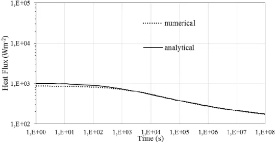
O’Sullivan, 2008]. ... 32 Figure 3: Example of model visualization with TOUGH2Viewe ... 45 Figure 4: comparison between the time functions proposed by Carslaw and Jaeger (dashed line) and Chiu and Thakur (circles). ... 51 Figure 5: Heat flux between the wellbore cell and the formation vs Time, comparison between the numerical and analytical results. ... 59 Figure 6: Absolute value of the difference between the temperature
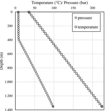
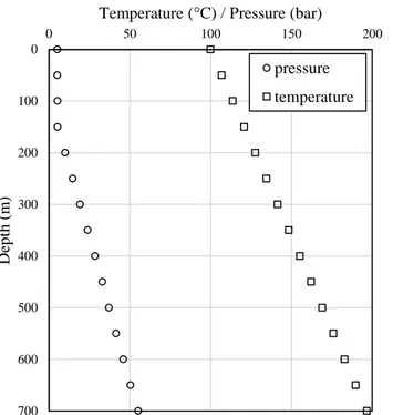
computed with the numerical approach and the temperature computed with the analytic approach for each time step. ... 60 Figure 7 Profile of pressure and temperature used as initial conditions for the simulation of well W2. ... 62 Figure 8: Initial condition for pressure and temperature for the production simulation of wellbore KD13. ... 63 Figure 9: Comparison between experimental data and simulation results for the flowing temperature profile of wellbore W2 after 11 hours of
production. ... 64 Figure 10: Comparison between experimental data and simulation results for the flowing pressure profile of wellbore W2 after 11 hours of production. . 64 Figure 11: Comparison between experimental data and simulation results for the flowing temperature profile of the wellbore KD13 after 100 hours of production. ... 65 Figure 12: Comparison between experimental data and simulation results for the flowing pressure profile of the wellbore KD13 after 100 hours of
production. ... 65 Figure 13: Conceptual model of the WW-1 well-reservoir system: well WW-1 and formation. ... 66 Figure 14: 2D vertical section of WW-01 wellbore –reservoir model. The main feed zones are the one with the lighter colors (yellow, green and cyan colors). The visualization of the model is performed by TOUGH2Viewer (Bonduà et al., 2012) ... 67 Figure 15: Initial pressure and temperature conditions assumed for the wellbore-reservoir model. ... 68 Figure 16: Comparison between simulated and measured mass rate. ... 70 Figure 17: Comparison between measured and simulated flowing pressure. The two set of data show a fairly good agreement. ... 71 Figure 18: Comparison between measured and flowing simulated
temperature. The two sets of data show a good agreement. ... 71 Figure 19: Flowing downhole pressure (800m and 1180 m depth) and WHP: simulated results compared with field measurements. ... 72
Figure 20 Measured and simulated production enthalpy. ... 73 Figure 21: Output curve: comparison between simulated results and
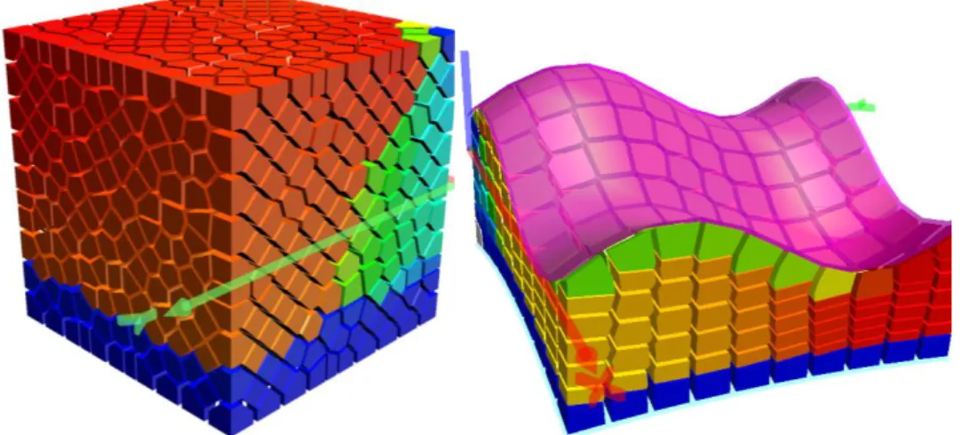
measured data. ... 74 Figure 22: 2D view of the gridded surface. Highlighted in red colour the position of the cluster of injection blocks. In green, the boundary block used as outlet of the system. ... 79 Figure 23: The 3D Voronoi grid (vertical exaggeration 5×), visualization by TOUGH2Viewer. ... 80 Figure 24: Grid and surfaces (purple wireframe) representing geological upper and bottom limits (vertical exaggeration 5×), visualization by
TOUGH2Viewer. ... 80 Figure 25: The same region gridded with: (a) regular discretization; (b) 3D Voronoi tessellation. The white wireframe represents the geological
boundary surface (vertical exaggeration 5×), visualization by Paraview. ... 81 Figure 26:Top view of non-aqueous phase saturation SNA after 106 years of
CO2 injection: (a) regular structured grid; (b) 3D Voronoi grid, as plotted by
Paraview. ... 82 Figure 27: Comparison of simulation results: total volume of gas vs time. 83 Figure 28: Comparison of simulation results: time steps vs. total simulated time. ... 83
List of Tables
Table 1: Primary variable sets in EWASG [Battistelli et al., 1997] ... 31 Table 2 Source code file for T2Well [Pan et al. 2011]. ... 52 Table 3: Production history of wellbore WW-01. ... 69 Table 4: Reservoir formation permeability (horizontal) as obtained by model calibration. ... 70 Table 5: Comparison of main characteristics of the regular structured grid and the 3D Voronoi grid. Volumes are in m3 and areas in m2. ... 82
Acknowledgements
I would like to thank the Geothermal Project Management Unit (PMU) of the Commonwealth of Dominica and ELC Electroconsult SpA for the permission to use well WW-01 field data.
Furthermore I would like to thank all the people who helped me with suggestions and inspirations: the Geothermal Research group of DICAM, Prof. Villiam Bortolotti, Prof. Paolo Berry, PhD Eng. Stefano Bonduà and PhD Eng. Carlo Cormio; Eng. Alfredo Battistelli of Saipem SpA, who collaborated to this work under the R&D project “Simulation of production tests with TOUGH2-T2Well”, and PhD Lehua Pan of the Lawrence Berkeley National Laboratory.
Introduction
In the last few decades, the demand of environmentally friendly energy is felt stronger. For “environmentally friendly energy” is meant the use of sources of energy not only less polluting, but also sustainable and renewable [Axelsson and Stefansson, 2003]. Geothermal energy, if correctly produced and managed, is one of these, and it is characterized by a particular versatility. In fact, it is used not only for the production of electrical energy (with temperature higher than approximately 150°C), but also in the case of lower temperature systems suitable for direct heat uses, such as space heating/cooling, greenhouses, aquaculture, etc. Italy was the first country in the world to develop the technology for the exploitation of geothermal energy (by Prince Piero Ginori Conti, 1904) and it is currently one of the world leaders in terms of electricity production from geothermal sources [Notiziario UGI, 2007; Bertani, 2015].
One of the goals concerning the geothermal exploitation activities is to keep the resource alive/available as much as possible, thus keeping the extraction of geothermal fluids compatible with the reservoir recharge, and taking advantage of the re-injection of the extracted fluids. During the exploitation of a geothermal reservoir it is therefore mandatory to be able to correctly plan the field development and perform a sound management of fluids production. This is a challenging activity that nowadays is essentially accomplished using numerical reservoir simulation. Geothermal numerical simulators, therefore, are of paramount importance to optimize the exploitation, for the
6 Introduction
characterization of geo-resources, to evaluate the economic sustainability of the project and estimate the environment impact.
It is, therefore, easy to understand that any effort dedicated to the improvement and optimization of numerical modelling and simulation is welcome, and this is the main objective of this study, particularly regarding the TOUGH family of codes [Pruess, 2004; Finsterle et al., 2014].
During the doctoral research work, many aspects of the geothermal numerical modeling and simulation were tackled and many specific software tools were used. In particular the improvement of the reservoir engineering activities has been a central point of the doctoral work. The main research work, therefore, deals with the use and improvement of T2Well (a coupled well-reservoir simulator based on TOUGH2, [Pan and Oldenburg, 2013] ) for the interpretation of geothermal well-tests. The dynamic P&T (pressure and temperature) logs and the pressure transient measurement during well-tests, unfortunately, are often incomplete, both for time saving and for issues related to the risk of loss of the logging tools, and this is a strong limitation in understanding of the reservoirs characteristics. A good way to solve the lack of these downhole data may be the use of coupled wellbore-reservoir flow simulation under transient conditions. In this way, it is possible to interpret the well-tests by means of simulations which allow analyzing the bottom and well-head measurements in an integrated approach, instead of analyzing them separately [Battistelli, 2016]. This can be done using, for instance, T2Well coupled with a proper Equation of State (EOS) module in order to allow the simulation of commonly exploited geothermal systems. While EWASG can be conveniently used to simulate geothermal reservoirs with temperatures from low to high, the applications described here below were focused on high temperature (or high enthalpy) reservoirs used for the generation of electrical energy. As high enthalpy geothermal fluids consist of mixtures of water, salts and non-condensable gases, supported by Eng. A. Battistelli and PhD L. Pan, T2Well was coupled with the EWASG module [Battistelli et al., 1997; Battistelli, 2012] to create the new code called
T2Well-EWASG. Furthermore, the analytical approach for the computation of heat exchange between the wellbore and the formation (option included in T2Well) was enhanced. The verification of T2Well-EWASG was accomplished by comparing analytical and numerical results concerning the heat exchange between the wellbore and the formation. The validation was obtained by reproducing flowing pressure and temperature logs taken from published literature and by using T2Well-EWASG for the interpretation of a short production test, performed on an exploratory well drilled in a recently discovered geothermal field.
Another important activity carried on during the doctoral work, concerns the improvement of pre- and post- processing tools specific for TOUGH2. Many efforts were done to modify the viewer TOUGH2Viewer [Bonduà et al., 2012] to work in conjunction with VORO2MESH [Bonduà et al., 2015]. In particular, TOUGH2Viewer was improved with new functionalities allowing managing fully unstructured 3D Voronoi grids created with VORO2MESH. The viewer was validated with a case study dealing with the migration of non-condensable gases in a deep sedimentary formation [Battistelli et al., 2015] using TOUGH2-TMGAS [Battistelli and Marcolini, 2009].
The thesis is structured as follows: It starts with a background chapter, where the topic of the research is described. Chapter 2 describes the TOUGH and T2Well software and the pre- and post-processor VORO2MESH and TOUGH2Viewer. Chapter 3 describes the T2Well-EWASG development and modifications; in chapter 4 the results of verification and validation of the software are provided. In chapter 5 the results of the application of TOUGH2Viewer and VORO2MESH are shown. Finally in chapter 6 conclusions and the hypothesis on future developments of the research are discussed.
1 Background
1.1 System, model, calibration and simulation
Defining the term process as a set of interactions, energy or material transformations and transmissions, aimed to obtain a certain goal, it is possible to define the system as a conglomerate of parts through which the process is realized. In other words, a system is a set of interacting parts, which constitute a single “body”, and that permits to the process to occur. The system behavior is characterized by a set of properties, which can be divided into two categories: the parameters, which usually are invariant system characteristics through time, and the variables, which are changing through the time as a consequent of the interactions between the different parts of the system and with the world external to the system. Usually, a real system is very difficult to analyze and study, because of the inability to proper evaluate the numerous system properties. For this reason, typically, the system is not studied directly, but using its simplified version which exclusively includes the crucial aspects of the system that concerns the problem analyzed. This simple version of the system is called model. There are different types of models: physical model, which can be scale models (scale representation of each element of the system) or analog model (representation of the system properties through different physical quantities), symbolic models (system representation in terms of symbols, which can be manipulated). The mathematical models, which describe the system in terms of equations and functional relations, are an example of symbolic models and can be
10 1 Background
distinguished in two categories: analytical and numerical models. The analytical models provide exact solutions, if any. The numerical models produce approximate solutions which are reasonably close to the expected results. Since in many cases it is impossible to obtain a solution of the analytical equations the numerical models are the only way to proper represent the system. As state before, the models are used in order to analyze and study the system, but in particular they allow two actions: the interpretation and the simulation. The interpretation is the procedure to interpret the output data of the system obtained by a specific stimulation of the system itself. The interpretation, therefore, is used in very important activities such as model calibration in primis, and in some extent also in sensitivity analysis and in the analysis of error propagation. In particular, the
model calibration allows to obtain the better values of the parameters of the
model (that also are parameters of the system) such that the model behavior is in agreement with that of the system. The sensitivity analysis allows to individuate what the parameters of the model are whose variations mostly impact on the output behavior of the model itself. Finally, the study of error
propagation permits to evaluate the influence of the uncertainty of the
parameters on the model results. The simulation is an activity which allows to use the model in order to obtain information about the behavior of the system, both in the original state evolution (natural state, before the exploitation of the system starts) and in its future evolution (during the exploitation period) [Bortolotti, 2013].
1.2 Numerical reservoir simulation
The multiphase multicomponent transport of mass and energy in porous and fractured rocks can be described by a set of partial differential mass and energy balance equations for which closed analytical solutions exist only for very simplified geometries, rock property distribution and thermodynamic
conditions. Thus, the set of partial differential equations suitable to describe the multiphase flow in geothermal reservoirs need to be solved with a numerical approach, by discretizing in space and time the partial differential equations in order to obtain an equivalent system of linear algebraic equations, which can then be solved with direct or iterative approaches. The numerical solution of complex differential equations becomes feasible with the diffusion of digital computers in the late 1960s. First adopted by the oil and gas industries, the numerical simulation becomes a common tool for the geothermal industry in the ‘80s. With the growth of computational power, the models gradually became more sophisticated, starting from very simple models, limited in details and characterized by, for example, single layer structure or 2D geometry, to achieve very detailed models, characterized, for example, by mesh with more than 106 grid blocks and layers that follow the geological structure of the formation [O’Sullivan et al., 2001].
Numerical modelling and simulation of geothermal reservoirs are essential tools in order to better optimize the resource exploitation and characterization. In fact, the simulation permits not only to study the reservoir before exploitation (i.e. the natural state modelling, that provides information that serve as the basis for exploitation models that may later be developed) but also to predict the possible future exploitation scenarios. The simulation is also useful to test the number and location for the wells, based upon a given generating capacity, to predict the longevity of the field according to a defined exploitation plan and to realize sensitivity studies [Bodvarsson, 1982]. Basically the numerical simulation consists in these main activities:
1. Collection of data, coming from geosciences, well production and reservoir engineering;
2. Review and interpretation of field data; 3. Development of the conceptual model; 4. Building of the numerical model;
5. Natural state calibration (by trial-and-error or with inverse simulation techniques);
12 1 Background
6. Matching of production history (by trial-and-error or with inverse simulation techniques);
7. Forecast of production and reinjection scenarios;
The first step involves the collection of all the needed data about the system in order to develop a conceptual model of the field. Collection and interpretation of field data is performed by experts in geosciences (geology, geophysics, geochemistry), taking advantage of both surface surveys and drilled wells, as well as by experts in well production and reservoir engineering. The construction of the conceptual model is a prerequisite of the simulation process because it is an outline that tries to connect all the available and useful information about the system and it requires the consultation of wide range of expertise: geologists, chemists, reservoir engineering and physicists [Grant M.A., Bixley P.F., 2011, cap 11]. Once the conceptual model has been developed, it is translated into the numerical model, in a format acceptable by the simulator (the software). Once the numerical model has been developed, it is possible to simulate the natural state condition. The simulation starts and goes on until the achievement of steady state conditions, which are usually assumed to be a proxy for the natural state. The natural state calibration consists in the adjustment of the model parameters by comparing the simulation results with the natural state conditions as depicted in the conceptual model, for example by comparing shut-in pressure and temperature profile measured in drilled wells with simulated results. The model parameters are changed until the differences between simulated and experimental data becomes lower than a target threshold. The history matching is performed using production/reinjection data: the model parameters are changed until the simulation results match the recorded behavior under exploitation of the actual reservoir. This last step is very important in order to determine the hydraulic condition of the formation [Grant M.A., Bixley P.F., 2011, cap 11]. De facto the realization of a model which reflect the actual system and that permits to predict different possible
exploration scenarios needs a continuous upgrade of data. Every experimental data, pressure and temperature logs, well test, etc, which become available with time, are important for the determination of the natural state and for the calibration and history matching of the model [Grant M.A., Bixley P.F., 2011, cap 11]. In this terms it can be stated that both the conceptual and numerical models need to be periodically updated during the development and exploitation phases to take advantage of new field observation acquired. Finally, once the model is calibrated, it is possible to use it in order to predict the possible future exploitation scenarios, in the process called forward simulation.
One of the main intent of the modeling activities is the evaluation of the spatial distribution of hydraulic properties and thermodynamic condition of the reservoir. Such characteristics play a key role in determining the production capacity of the wells and the reservoir behavior under exploitation. Common well-tests performed for the evaluation of the hydraulic properties are: production testing, shut-in and flowing temperature and pressure logging (either during injection and production and during and after drilling of the well), down-hole pressure transient measurements. For a more detailed description of the objectives and characteristics of well-test the reader is referred to Grant and Bixley 2011.
Production tests serve for the determination of the fluid enthalpy and to obtain the deliverability curve (flow rate versus the well head pressure). The P&T (pressure and temperature) logs, recorded both during injection and production, allow to locate the feed-zone, the thermodynamic properties of the feed-zone fluids and they are usually used for the calibration of the model. Pressure transient analysis requires the disturbance of the pressure state of the reservoir by production or injection and measuring the resulting pressure transients. They are performed to assess the principal hydrological parameters of the formation near the well, such as [Axelsson, 2013]:
formation permeability-thickness; formation storage coefficient;
14 1 Background
skin factor of the well; wellbore storage coefficient.
1.2.2 Reservoir Simulators
The first geothermal simulator has been developed in the 1970s for the study of the Wairakei geothermal field [O’Sullivan et al., 2009]. Development of geothermal numerical reservoir simulators at Lawrence Berkeley Laboratory (now LBNL) started in 1975 with the first version of SHAFT [Lasseter et al., 1975] and continued with the SHAFT78 and SHAFT79 release [Pruess, 1988]. In 1977 Faust and Mercer realized a model that can simulate two-dimensional flow of compressed water, two-phase mixture and super-heated steam over a temperature range between 10° and 300°C [Faust and Mercer, 1977]. In 1982 Bodvarsson realized PT (pressure-temperature) a simulator for three-dimensional mass and energy transport in a liquid-saturated medium, based on Integrated Finite Difference Methods (IFDM). PT also computes the deformation of the medium using the one-dimension consolidation theory of Terzaghi [Bodvarsson, 1982]. AQUA [Hu S., 1994; Hu B., 1995] is a software developed by Vatnaskil Consulting Engineers, 1990, to modelling the groundwater fluid flow and transport, based on the Galerkin finite element method. Aqua3D is a Galerkin finite-element numerical modelling software used to model 3D groundwater and contaminant transport, sell by Vatnaskil consulting engineers since 1997 [Vatnaskil, 1997]. HYDROTHERM [Hayba and Ingebritsen, 1994] is a finite-difference model describing three-dimensional, multiphase flow of pure water and heat at near-critical and supercritical temperatures (up to 1200°C). It has been developed as an extension of multiphase geothermal models produced by Faust and Mercer in the 1970s. This kind of multiphase model are needed in study related cooling plutons, crustal-scale heat transfer and volcanic systems with shallow intrusion.
Common simulators are STAR [Pritchett, 1995], a simulator for multiphase, multicomponent transport of fluid mass and heat in three-dimensional geologic media, and TETRAD [Vinsome and Shook, 1993], which require regular rectangular meshes. In this work was used one of the most popular software for geothermal numerical modeling, TOUGH2 [Pruess et al., 1999].
1.2.2.1 Brief overview on TOUGH family of codes
TOUGH is an acronym, which stand for “Transport Of Unsaturated Groundwater and Heat”. The most famous software of the TOUGH family of codes is TOUGH2. TOUGH2 is a numerical simulator for non-isothermal flows of multicomponent, multiphase fluids in one, two, and three-dimensional porous and fractured media. In addition to being widely used for geothermal simulations, TOUGH2 is used also for modelling of nuclear waste disposal, environmental remediation and geological carbon storage. TOUGH2 is used not only for academic purpose but also for private industrial works and also by government organization [Finsterle et al. 2014]. TOUGH2 is the result of about forty years of research at the Lawrence Berkeley National Laboratory (LBNL). After SHAFT, the first prototype developed in mid ‘70s [Pruess, 1988], in the 1980s, LBNL developed MULKOM, a modular architecture for simulating the flow of multicomponent, multiphase fluids and heat in permeable (porous or fractured) media [Pruess, 2004]. In 1987 a specialized version of MULKOM was released to the public under the name of TOUGH [Pruess, 1987], that was able to handle two-phase flow of water-air mixture. Subsequently, in 1991 TOUGH2 [Pruess, 1991], a more global set of MULKOM modules, was released, followed by TOUGH2 version 2.0 [Pruess et al., 1999] in 1999. Unlike STAR and TETRAD, TOUGH2 is able to handle unstructured meshes. TOUGH2 is structured by a modular architecture: there is a core module dedicated to assemble and
16 1 Background
iteratively solve the flow equations and an Equation Of State (EOS) module, which is dedicated to the description of the specific thermophysical properties of fluid mixtures involved in the problems.TOUGH2 V.2.0 is written in FORTRAN 77 and requires as input a set of ASCII files (whose manipulation is not easy without specific pre-processor software, especially in the case of full field simulations) defining the numerical model and its use in the simulation process. A more detailed description of TOUGH2 is proposed in chapter 2.
Other relevant tools from the TOUGH family of codes are T2VOC [Falta et al., 1995] and TMVOC [Pruess and Battistelli, 2002] and TMVOCBio [Battistelli, 2004] dedicated to study environmental contamination problems in presence of non-aqueous phase liquids. TOUGHREACT [Xu and Pruess, 2001, Xu et al., 2004] was realized for the modeling of non-isothermal multiphase flow and geochemical transport (reactive transport including equilibrium and kinetic mineral dissolution and precipitation, chemically active gases, intra-aqueous and sorption reaction kinetics and biodegradation). iTOUGH2 is an extension of TOUGH2 that allows inverse modeling, parameter estimation, sensitivity analysis, and uncertainty propagation analysis [Finsterle, 2007]. TOUGH-FLAC [Rutqvist et al., 2002] is the coupling of TOUGH2 and FLAC3D [Itasca Consulting Group Inc., 1997] and it allows the integrating simulation of geomechanics deformations and fluid and heat flow in porous media. TOUGH-MP [Zhang et al., 2008] is the TOUGH2 version for the massively parallel computing. TOUGH+ v1.5 [Moridis and Pruess, 2014] is a TOUGH2 successor, which uses dynamic memory allocation and is coded in FORTRAN 95/2003. TOUGH 2.1 [Pruess et al. 2012] is the last version of TOUGH2, with a restructured core, several bug fixes and support to additional EOS modules such as T2VOC, EOS7CA, ECO2N, ECO2M, and TMVOC.
1.2.2.2 Pre- and Post-processing tools for TOUGH
family of codes
As mentioned in the previous section, TOUGH2 does not have a native Graphical User Interface (GUI), so over time many efforts have been spent in order to manage input and output file, both by software houses and by scientific research group. A list of software tools developed by scientific group is: MulGeom [O’Sullivan and Bullivant, 1995], GeoCad [Burnell et al., 2003], G*Base [Sato et al., 2003], Simple Geothermal Modelling Environment [Tanaka and Itoi, 2010], TOUGHER [Li et al., 2011], PyTOUGH [Croucher, 2011; Wellmann et al., 2012]. Whereas a commercial list is: Petrasim [Alcot et al., 2006], WinGridder [Pan, 2003], mView [Avis et al., 2012] and Leapfrog [Newson et al., 2012]. In order to better manage the information required to realize the input files and to easily realize locally refined Voronoi grid, the geothermal research group of DICAM has realized TOUGH2GIS [Berry et al., 2014] a GIS-based pre-processor, and TOUGH2Viewer [Bonduá et al., 2012], a 3D visualization and post-processing tool, recently improved to visualize fully Voronoi 3D grid. To create fully Voronoi [Voronoi, 1908; Aurenhamer, 1991] 3D grids the geothermal research group of DICAM has developed VORO2MESH [Bonduá et al., 2015] a new software coded in C++, based on the voro++ library [Rycroft, 2009].
1.2.3 Coupled Wellbore-Reservoir Simulators
Since the 1980s, many efforts have been made in order to couple wellbore and reservoir simulators. The importance of the simulation of coupled wellbore-reservoir fluid flow lies in the fact that the flow inside the geothermal well cannot be considered isolated, but it must be considered in
18 1 Background
conjunction with the flow of fluid in the reservoir [DiPippo, 2008]. This approach leads to a more reliable modelling of the phenomena involved in the exploitation of the resource.
One of the first coupled software is due to Miller (1980), who developed a transient-wellbore code, WELBORE. The code allows the simulation of one-dimensional, two-phase, non-isothermal fluid flow in a wellbore coupled with the simulation of single-phase radial flow in the reservoir [Miller, 1980]. Murray and Gunn (1993) proposed a coupled wellbore-reservoir simulator composed by TETRAD and WELLSIM [Gunn and Freeston, 1991; Freeston and Gunn, 1993]. The latest is a steady-state wellbore simulator, which includes three codes: WFSA (for the simulation in presence of dissolved solids, multiple feed-zones and fluid-rock heat exchange), WFSB (dedicated to the simulation of gaseous well) and STFLOW (built to model saturated and superheated steam typical of wellbore located in vapor-dominated zones). TETRAD-WELLSIM coupling works by means of lookup table of wellbore pressure generated by WELLSIM given as input to TETRAD. In a paper of the 1995, Hadgu et al. describe the coupling of TOUGH and the steady-state wellbore simulator WFSA. In this way they were able to model the flow of geothermal brine both in the wellbore and in the reservoir, by using a new module, called COUPLE, which allowed TOUGH to call WSFA as a subroutine. Bhat et al. (2005) coupled TOUGH2 with the steady-state wellbore simulator HOLA [Björnsson, 1987]. HOLA is designed for the modeling of multi-feed zone in a wellbore of pure water, characterized by one or two phase flow. Modified versions of HOLA exist: GWELL, for the modeling of carbon mixture and GWNACL for the modeling of water-salt mixture. Similar to the work of Hadgu et al., Bhat et al. integrated HOLA as a subroutine of TOUGH [Bhat et al., 2005]. Tokita et al., presented in 2005 a method developed to predict the effects on a reservoir due to exploitation using a new simulator resulting by the coupling of a reservoir simulator, TOUGH2, a steady-state multi-feed zone wellbore simulator, MULFEWS [Tokita and Itoi, 2004], and a two-phase pipeline network simulator. The
simulator was used to forecast the middle-term power output of the Hatchobaru power plant in Japan. Marcolini and Battistelli [2012] developed wellbore flow modeling capabilities inside TOUGH2 by coding the solution of steady state mass, momentum and energy equations for the wellbore on deliverability option already available in TOUGH2. This code modification, limited to EOS1 and EOS2 modules, was addressed to the modeling of coupled wellbore-reservoir flow in full field geothermal reservoir simulations. Gudmndsdottir et al. (2012) developed a coupled wellbore-reservoir simulator using TOUGH2 and FloWell [Gudmndsdottir et al., 2012; Gudmndsdottir and Jonsson, 2015]. FloWell is a steady-state wellbore simulator dedicated to model liquid, two-phase and superheated steam flows in geothermal wells, and was part of a research project whose aim was to evaluate the well performance and the state of the reservoir using wellhead condition and inverse modeling. To address the need to simulate the coupled wellbore-reservoir flow, Pan and Oldenburg (2013) developed T2Well, a numerical simulator for non-isothermal, multiphase, and multi-component transient coupled wellbore-reservoir flow modeling [Pan and Oldenburg, 2013]. T2Well is the coupled wellbore-reservoir simulator used in this work. T2Well expands the numerical reservoir simulator TOUGH2 capabilities in order to compute the flow in both the wellbore and the reservoir by introducing a special wellbore sub-domain into the numerical grid. The wellbore flow is simulated using the Drift Flux Model [Zuber and Findlay, 1965]. As TOUGH2, T2Well can be used with different EOS in order to describe different fluid mixtures. Up to now it has been used with ECO2N [Pruess, 2005] for applications related to CO2 sequestration [Hu et al., 2012],
with ECO2H [Pan et al., 2015] for enhanced geothermal system simulations, with EOS7C [Oldenburg et al., 2013] for applications related to compressed air energy storage, and with EOIL for the modeling of Macondo well blowout [Oldenburg et al., 2011]. The heat exchanges between wellbore and the surrounding formation can be simulated numerically or, alternatively
20 1 Background
calculated with the analytical Ramey’s method [Ramey, 1962] or the Zhang’s convolution method [Zhang et al., 2011].
Since T2Well is simulator, which combine the capabilities and the benefits of TOUGH2 and allows the coupled wellbore-reservoir flow simulation under transient condition, it results that it is the eligible tool for the interpretation of well-tests, allowing the simulation of bottom and well-head measurement in an integrated approach.
2 TOUGH2, T2Well, TOUGH2Viewer and
VORO2MESH
2.1 TOUGH2
TOUGH2 is a numerical simulator program dedicated to multi-dimensional fluid and heat flow, characterized by multi-component and multiphase fluid mixture, in porous and fractured media. TOUGH2 is widely used in industrial and academic world and in different areas such as geothermal reservoir engineering, radioactive waste disposal, CO2 sequestration, environmental
assessment, etc.
TOUGH2 is characterized by a modular structure, with a main module dedicated to the assembling and solution of the flow equation that provides the primary variables to the EOS module and receives from it the values of secondary parameters according to the thermodynamic relation implemented in the EOS module.
There are different EOS modules that describe different thermodynamic systems: EOS1 is dedicated to water and water with tracer, EOS2 describe the thermodynamic equation for a mixture of water and CO2, etc. The
available EOS up to now are:
- EOS1: water, water with tracer, heat; - EOS2: water, CO2, Heat;
24 TOUGH2, T2Well, TOUGH2Viewer and VORO2MESH
- EOS4:water, air, with VPL, heat; - EOS5:water, hydrogen, heat; - EOS7:water, brine, air, heat;
- EOS7CA: water, brine, NCG (CO2, N2 or CH4), gas tracer, air, heat;
- EOS7R: water, brine, air, parent-daughter radionuclides, heat; - EOS8: water, air, oil;
- EOS9: Water (Richards’equation); - T2VOC: Water, air, voc, heat;
- EWASG: Water, salt (NaCl), NCG (includes precipitation and dissolution, with porosity and permeability change; optional treatment of VPL effects), heat;
- ECO2N:water, brine, CO2;
- ECO2M: water, brine, CO2 (multiphase);
- TMVOC: water, VOCs, NCGs; - T2DM: 2D dispersion module.
This modular structure gives TOUGH2 both the ability to simulate different thermodynamic situations and the flexibility to be applied to different area of interest. The set of primary variables depends on the type of EOS module chosen, for example in EOS2 the primary variables are pressure, temperature and CO2 partial pressure, whereas in EWASG, the primary variables are
pressure, salt mass fraction, NCG mass fraction and temperature.
The values of the primary variables are used in the EOS module to compute the secondary parameters, such as density, viscosity, enthalpy, etc. that are used to assemble the mass and energy balance equations.
In the next two paragraphs a survey of the fundamental equation used by TOUGH2 is presented, as it is described by Pruess et al., 1999, in the TOUGH2 v 2.0 manual.
2.1.1 Mass and energy balance
For each grid-block of the numerical model, TOUGH2 resolves the mass-energy balance equation:
n n n k k k n n n V V d M dV F n d q dV dt
(2.1)Where Vn and Γn are respectively the volume and the surrounding surface of
the element, n is the normal vector to the surface dΓn and Fk is the flux term. On the left side of the equation (2.1) there is the accumulation term, Mk that represents the mass (or energy) per volume. On the right side there are two integrals, the first take account of the mass (or heat) flux and the second represents the source and sink contributes. In the mass-casek1, 2,...,NK, where NK is the number of mass component. In the case of energy balance
1
kNK .
In the mass balance of a system characterized by more than one component in several phases, the accumulation term takes the form:
k k
M S X
(2.2)In which the porosity () is multiplied for the sum of each phase contribute of a k-component. Sβ, ρβ and Xβk are respectively the saturation, the density and the mass fraction of the phase β. The term, Fk, is equal to the sum all over the phases of the flux term of each phase weighted by the mass fraction
( k X): k k F X F
(2.3)Where Fβ is computed using the Darcy’s law:
r k F v k P g (2.4)26 TOUGH2, T2Well, TOUGH2Viewer and VORO2MESH
In which compare the Darcy’s velocityv of the phase β, the absolute permeability k, the relative permeability krβ, the viscosity coefficient, the fluid pressure P related to the phase β and the gravity vectorg. In this case
the sink and source contribute is a mass rate per volume.
In the energy balance, the heat accumulation is given by two contributes:
1 1 KN R R M C T S u
(2.5)The first contribute takes into account the matrix heat provision,
Ris the rock density, CR the rock specific heat and T is the rock temperature. The second contribute stands for the heat of each phase, where u is the specific internal energy of the phase β.Heat flux include conductive (Fourier’s law) and convective components:
1 NK F T h F
(2.6)Where his the specific enthalpy of the phase β, T is the temperature and
is the thermal conductivity.
2.1.2 Space and time discretization
TOUGH2 is based on the integral finite difference method (IFDM). Under this point of view, the accumulation term of equation (2.1) becomes:
n k k n n n V M dV V M
(2.7) where k nM is the average value of Mkin the volume Vn and similarly for the sink and source term:
n k k n n n V q dV V q
(2.8) with k nThe surface integral can be written as: n k n nm nm m F n d A F
(2.9)In which Fnmis the average value of the normal component of the flux Fk to
the surfaceAnmbetween the element Vn and Vm. In this way, equation (2.1) can be rewritten as:
1 k k k n nm nm n m n d M A F q dt V
(2.10)Time is discretized as a first-order finite difference and the flux term is processed with ‘fully implicit’ method. This means that the flux term and the sink and source contribution, on the right side of equation (2.10), are expressed in terms of the unknown thermodynamic parameters at the time step t1 t t. This method ensures numerical stability for the calculation of multiphase flow. The time discretization is then represented by the following set of coupled non-linear, algebraic equations:
k, 1 k, 1 k, k, 1 k, 1 0 n n n nm nm n n m n t R M M A F V q V
(2.11) In which each k, 1 nR is the residual corresponding to the kth equation (k=1, 2…
NEQ; NEQ= NK+1; NK is the number of fluid components), related to the nth
element, at the t 1 time step. For each grid block of volume Vn there are NEQ equations. In this way for a system characterized by NEL grid blocks, equation (2.11) represents a set of NEL NEQ coupled non-linear equations with NEL NEQ unknown independent primary variables which define the state of the flow system at the time step tk1. The resolution of these equations is made using Newton-Raphson iteration.
28 TOUGH2, T2Well, TOUGH2Viewer and VORO2MESH
2.1.3 Brief input file description
The TOUGH2 input file is composed by one or more ASCII data files, which describe the rocks properties of the system, the geometry of the mesh, the computational parameters, the initial conditions, etc. All these data have to be provided following a fixed format. The information are organized in blocks, identified by fixed keywords, and up to 80 characters per records compose them (see Figure 1). TOUGH2 adopts the standard metric (SI) unit (meters, seconds, kilograms) with the temperature expressed in Celsius degrees.
Figure 1: Example of TOUGH2 input file.
Here I supply a brief description of the main keywords. For a detailed description of the format and for a complete description on how to write the TOUGH2 input file, the reader is referred to the TOUGH2 v.2.0 manual [Pruess et al., 1999]. The keyword ROCKS describes the rock types providing
the hydrogeologic parameters (porosity, permeability, heat conductivity, specific heat, etc.). The keywords ELEME and CONNE provide the geometric information about the mesh (nodes coordinates, interfaces areas, etc), and in ELEME it is also specified the rock type for each grid block. The keyword MULTI is used in order to specify the number of fluid components and balance equations per grid block. SELEC is used to provide thermophysical property data. PARAM is the keyword dedicated to define the computational parameters, such as time stepping, simulated time and program options. Using the keyword GENER it is possible to define the sinks and sources. With the keywords INCON and INDOM it is possible to specified the initial condition.
2.1.4 EWASG EOS MODULE
EWASG (Equation-of-state for Water, Salt and Gas) is a EOS module for TOUGH2 V.2.0 used primarily for modeling hydrothermal systems containing dissolved solids and one non-condensable gas (NCG) such as CO2,
CH4, H2S, N2 and H2 [Battistelli et al., 1997]. Such components are typical of
geothermal reservoir. The limits of validity of thermodynamic correlations implemented in EWASG are up to 350°C and up to 1000 bar for H2
O-NaCl-NCG mixtures [Battistelli et al., 2012], with the limitation of low to moderate NCG partial pressures. In literature, it is possible to find several applications of the EOS EWASG. Battistelli and Nagy (2000) used it to evaluate the exploitation of geothermal resources in Skierniewice area in Poland characterized by high salinity aquifer at a temperature equal to 70°C. Battistelli et al. (2002) tested a conceptual model of Dubti geothermal field (Ethiopia) by using a simple 3D model. Crestaz et al. (2002) applied EWASG for the modeling of sea water intrusion in coastal plains of the Dominican Republic. Weisbrod et al. (2005) modeled the salt accumulation and precipitation due to water evaporation from soil fractures. Battistelli and Marcolini (2012) used EWASG supported by the pre- and post-processor
30 TOUGH2, T2Well, TOUGH2Viewer and VORO2MESH
Petrasim to model the natural state and simulate the production forecast for Lumut Balai geothermal field, Indonesia. Battistelli (2013) used EWASG supported by Petrasim to model the natural state and simulate the production forecast for Patuha geothermal field, Indonesia. Sirait et al. (2015) used EWASG supported by Petrasim to model the natural state and simulate the production forecast for the Dieng field, Indonesia. Other researchs are related to the investigation of the use of TOUGH2-EWASG for the modelling of halite formation in natural gas storage aquifers [Lorenz and Muller, 2003] and for the numerical simulation of salt water injection into a depleted geothermal reservoir [Calore and Battistelli, 2003; Geloni and Battistelli, 2010]. Flint and Ellett (2003) employed EWASG to model the artificial recharge of an aquifer in California, USA. Pruess et al. (2002) applied EWASG to study the hydrogeological processes developing outside the buried tanks and containing high level nuclear wastes at Hanford site, USA. Esposito and Augustine (2014) used EWASG to model the exploitation of a geopressured resource located in Texas, USA. Purwanto and Kaya (2015) modeled geothermal reservoirs in Waiotapu-Waikite-Reporoa areas, New Zealand. Blanco Martìn et al. (2015) applied EWASG with the TOUGH-FLAC simulator to model the coupled hydrodynamic and geomechanical processes in a generic salt repository for heat-generating nuclear wastes. Ratouis et al. (2016) performed simulations of the Rotorua geothermal field (New Zealand).
2.1.4.1 Thermodynamic description
A detailed description of the thermodynamic capability of EWASG is proposed by Battistelli et al. in a paper published in 1997 [Battistelli et al., 1997]. Here the aim is to outline the main features, the improvements
dedicated to update EWASG in the last years [Battistelli, 2012] and the characteristic correlations.
As stated before, EWASG describes a system composed by tree phases (solid, liquid and gas) and neglecting the case of single solid phase, the remaining combination are six. Table 1, created starting from Battistelli et al., 1997, lists the primary variables for each thermodynamic state. The code is able to determine the passage from a thermodynamic state to another by controlling the main thermodynamic variables of the system. For example, in the case of liquid conditions, the code checks the value of the pressure comparing it with the boiling pressure curve. Solid salt phase pops up if the salt mass fraction in the liquid phase exceeds the solubility of solid salt. In gas conditions it is possible for liquid to appear only if its partial pressure is greater than the vapour saturated brine pressure.
Table 1: Primary variable sets in EWASG [Battistelli et al., 1997] Thermodynamic
condition
Primary variables
1 2 3 4
Liquid Total pressure (liquid)
Salt mass fraction (liquid)
NCG mass
fraction (liquid) Temperature Gas Total pressure
(gas)
Salt mass fraction (gas)
NCG mass
fraction (gas) Temperature Liquid + gas Total pressure
(gas)
Salt mass fraction (liquid)
Gas phase
saturation Temperature Liquid + solid Total pressure
(liquid) Solid saturation
NCG mass
fraction (liquid) Temperature Gas + solid Total pressure
(gas) Solid saturation
NCG mass
fraction (gas) Temperature Liquid + gas + solid Total pressure
(gas) Solid saturation
Gas phase
saturation Temperature
Finally, in the case of liquid-gas mixture the code examines the gas phase saturation (SG): in a two-phase fluid system, when SG becomes equal or
32 TOUGH2, T2Well, TOUGH2Viewer and VORO2MESH
liquid phase. If the gas saturation assumes a negative value then the gas phase disappears and the single-liquid phase takes place. In the original version of EWASG pure water properties were computed using the International Formulation Committee correlations [IFC, 1967], but in the latest version these properties are computed using the IAPWS-IF97 correlations [Battistelli, 2012]. Different correlations for computing saturation pressure, density and internal energy for liquid water and steam are defined according to the different regions of the phase diagram (shown in Figure 2): liquid, vapour, super-critical and two-phase.
Figure 2: Phase-pressure diagram for the IAPWS-97 [Croucher and O’Sullivan, 2008].
In region 1 the thermodynamic conditions are those of the liquid phase, up to 350°C and 1000 bar. Region 2 describes the thermodynamic condition of steam up to 800°C and 1000 bar. Region 4 describes the two-phase condition up to the critical point (T = 373,946 °C, P = 220,64 bar). Finally, region3, which describes the supercritical condition is not taken into account in EWASG. The correlations for the dynamic viscosity of water and steam are taken from the IAPWS 2008, which provide more accurate viscosity values at high temperature [Battistelli, 2012].
In the latest version of EWASG, some correlations dedicated to the water-salt mixtures, like brine density, brine enthalpy and halite density, are computed using Driesner (2007). For brine density and enthalpy, Driesner proposes correlations between the water-salt solution and a reference substance, i.e. pure water. Starting from the temperature and salt mass fraction of the brine it is possible to compute the temperature TV* at which the pure water has the
same molar volume. Then the pure water density is determined by IAPWS-97 correlation. Finally, the brine density is computed with the following expression [Battistelli, 2012]:
2
2 * , , , brine brine NaCl H O V H O PM T P X T P PM (2.12)Where PMH O2 is the molecular weight of pure water and PMbrine is the brine
molecular weight, computed from the salt mass fraction and
2
H O
is the pure water density. Driesner proposes a similar approach for the determination of brine enthalpy: by computing the temperature TH* (function of pressure and
salinity) at which the pure water has the same enthalpy of the brine [Driesner, 2007]:
, ,
2
*,
brine NaCl H O H
h T P X h T P (2.13)
A linear relation with the pressure provides the halite density:
0
halite halite lP
(2.14)
Where
halite0 , the halite density at zero pressure and it is temperature dependent. l is a temperature dependent parameter. The correlations cover a range of temperature up to 350°C, with a minor error up to 370°C, the pressure can become up to 1000 bar and the NaCl concentration up to saturation. These correlations are coded into the DRIESNER subroutine. The halite solubility is computed as a function of temperature, T, using a correlation by Potter and quoted by Chou (1987):2
26.218 0.0072 0.000106
100
T T
34 TOUGH2, T2Well, TOUGH2Viewer and VORO2MESH
This expression is valid for temperature between 0°C and 800°C and it is coded into HALITE subroutine. Previously the enthalpy of halite was computed by integrating the specific heat provided by Silvester and Pitzer (1976), in the latest version of EWASG, the halite enthalpy is computed using the correlation for the specific heat given by Driesner (2007) in which it is function of both pressure and temperature:
2 2, 0 2 1 , 3 2 , 3 4
P halite triple NaCl triple NaCl
c b b TT b TT b P b P (2.16) where b0, b1and b2are known constants, b3and b4are obtained solving polynomials with respect the temperature. The integration of eq. (2.16) is made considering the halite enthalpy at triple point of halite as reference state (0 J/kg for enthalpy of pure liquid water at the triple point).
The brine vapour pressure is computed using a correlation by Haas (1976), coded into subroutine SATB. It is based upon the observation of Othmer et al., 1968a and 1968b, that the temperature of the brine (Tx) and the temperature of the pure water (T0) at the same pressure are related by the following expression: 1 ln 0 x x T D D T T e (2.17)
Where D and D1 are salt concentration polynomials. By computing the equivalent temperature for pure water, it is then possible to determine the saturation pressure using the pure water subroutine (SAT).
In regard to carbon dioxide component, density and enthalpy are computed using equation from Sutton and McNabb (1977). In particular, for the specific enthalpy they proposed the following expression:
2 6 10 8 7 10/3 1.667 10 1542 794800 log 0.3571 1 7.576 10 4.135 10 / 100 CO h T T P P T T (2.18)Where T is the temperature (in Kelvin), P is the pressure (in Pascal).
The dynamic viscosity of carbon dioxide is calculated using the correlation by Pritchett et al (1981):
2 3 4
80(P) 1(P) T 2(P) T 3(P) T 4(P) T 10
E E E E E
(2.19)
WhereE0, E1, E2, E3 and E4 are pressure dependent coefficients and Tis the temperature (in Celsius). This correlation is coded into VISGAS subroutine.
2.2 T2Well
As mentioned in the introduction section, T2Well is an extension of TOUGH2, which provides additional capabilities to calculate the flow in wellbore and reservoir. By introducing a special wellbore sub-domain into the numerical grid, denoted by “w” or “x” as initial letter, the code is able to compute the wellbore flow using the Drift Flux Model (DFM) [Zuber and Findlay, 1965]. In the next subparagraph, following the T2Well Manual by Pan et al. 2011, it is reported a survey of the fundamental equation solved by T2Well, a summary of the DFM, a brief description of both the discretized equations and of the analytical heat exchange.
2.2.1 Mass and energy balance
The equation for the mass and energy conservation have the same structure as in TOUGH2, eq.2.1: n n n k k k n n n V V d M dV F n d q dV dt
(2.20)The main difference from the equations used by TOUGH2 for the porous media are in the energy flux, energy accumulation and in the computation of phase velocity. Since the DFM implemented in T2Well is related to the
36 TOUGH2, T2Well, TOUGH2Viewer and VORO2MESH
motion of two phases, the mass accumulation term for the wellbore cells can be written as [Pan et al. 2011]:
1 2 k k k k G G G L L L M S X S X S X k and
(2.21)Where Xk denotes the mass fraction of the k component in the phase β,
is the density of the phase β and Sstands for the local saturation of the phaseβ. The local saturation is computed for both the phases with the sequent
relation: G G G G L A A S A A A (2.22)
Where A is the cross-sectional area and AG and AL are respectively the cross-sectional area occupied by the gas and the liquid phase over the cross section at a given elevation.
The energy accumulation term for wellbore cells is given by:
1 3 1 2 2 KN M M S u v
(2.23)Where uis the internal energy, 1 2
2v is the kinetic energy, both are per unit
mass, of the phase β.
For what concern the flow term, the relation to compute the total advective mass transport for the component k in one dimension is:
(A X S ) (A X S ) 1 k k k G G GvG L L LvL F A z z (2.24)
Where z is the coordinate along the wellbore.
The energy flux includes contributes due to advection, kinetic energy, potential energy and lateral wellbore heat loss/gain, and in one dimension can be written as:
2 1 3 1 cos 2 KN ex v T F F A S v h S v g Q z A z
(2.25)Here h denotes the specific enthalpy of the fluid phase β, g is the module of gravitational acceleration and Qexis the terms that take into account for the heat loss or gain of wellbore per unit length of wellbore (optional if the surrounding formation is not represented in the numerical model). is the angle between wellbore section and vertical direction. T is the temperature and λ is the area-averaged thermal conductivity of the wellbore.
The velocity of both phases, gas and liquid, are computed using the DFM, which is described in the next paragraph.
2.2.2 Drift Flux Model
First developed by Zuber and Findlay (1965), the Drift Flux Model represent a valid alternative for the study of two-phase flow in a pipe, in particular for the determination of the phase velocities, without solving the momentum equation for each phase.
The Drift Flux Model is based on the empirical constitutive relationship (all variables in the following development have to be considered as area-averaged or assumed to be constant over a cross-section):
Which stands that the gas velocityvG, can be related to the volumetric flux of
the mixture j, and the drift velocity of the gas,vd, via the parameter C0, named profile parameter, which takes in account for the effect of local gas saturation and velocity profiles over the pipe cross-section [Pan et al, 2011]. By definition, the volumetric flux of the mixture is:
Where vLis the liquid velocity and, combining the equations 2.26 and 2.27, it can be determined as:
0 G d v C j v (2.26) (1 ) v G G G L jS v S (2.27)
![Table 1: Primary variable sets in EWASG [Battistelli et al., 1997]](https://thumb-eu.123doks.com/thumbv2/123dokorg/8136575.125968/43.892.191.747.611.950/table-primary-variable-sets-in-ewasg-battistelli-al.webp)
![Figure 2: Phase-pressure diagram for the IAPWS-97 [Croucher and O’Sullivan, 2008].](https://thumb-eu.123doks.com/thumbv2/123dokorg/8136575.125968/44.892.184.648.438.782/figure-phase-pressure-diagram-iapws-croucher-o-sullivan.webp)
![Table 2 Source code file for T2Well [Pan et al. 2011].](https://thumb-eu.123doks.com/thumbv2/123dokorg/8136575.125968/64.892.145.706.352.877/table-source-code-file-t-well-pan-et.webp)