The Impact of Transaction Costs on Turnover and Asset Prices; The Cases of Sweden’s and Finland’s Security
Transaction Tax Reductions.
by
Peter L. Swan and Joakim Westerholm
Introduction
There is an ongoing debate on the effect of transaction taxes on financial markets. Several papers recommend the introduction of a security transaction tax [STT] to curb “excessive” short-term trading and to there by reduce “excess” volatility in the prices of financial assets. Traditional finance theory assumes the absence of benefits from trading, namely liquidity, when transaction costs are incorporated. Commonly a model is specified assuming no transaction costs and then these costs are subtracted from cash flows without further refinement of the underlying model. However, financial assets cannot be valued correctly if the costs of providing liquidity, i.e. transaction costs, are incorporated in the model while the benefits of liquidity are excluded. A companion paper by Swan (1999) challenges traditional theory and presents a new capital asset pricing model that incorporates transaction costs and the benefits of endogenous trading. In this paper we test the endogenous trading model in the context of a study of the effects of STT changes. The reason we do this is because the STT change is an exogenous event with a major impact on transaction
costs and thus an appropriate environment in which to study the effects of such changes on both turnover and asset prices.
To add current empirically based information to the discussion on the effects of STT we study the partial and then complete abolition of the STT in Sweden in 1991 and the abolition of the STT in Finland in 1992. We thus continue the work started by Umlauf (1993). We also add empirical evidence to the discussion on pricing of liquidity started by Amihud and Mendelsson (1986b). The most recent empirical evidence relevant for this discussion is presented by Chalmers and Kadlec (1998). The purpose of this paper is to test the Swan (1999) model of asset pricing together with a related turnover model, and to apply these models to the STT changes in Sweden and Finland.
When we use information available to all market participants up to the day before the change in STT we find that we can predict the impact with considerable accuracy. In Sweden the turnover rate (value of shares traded to market capitalization) is predicted to increase from 18 to 22 percent following the first reduction in STT and from 22 to 30 percent following the final abolition of STT. Asset prices are predicted to increase by 7.5 percent following the first STT reduction and 9.7 percent as a result of the second reduction. In Finland the turnover rate is predicted to increase from 10 to 15 percent following the abolition of STT change while prices are predicted to rise by 6.6 percent. These predicted changes are also observed in the markets with some of the price changes taking place at announcement of the STT change and the turnover increases within 8 months for Finland and 14.5 months
explanations for the price increases. When we include data pre and post STT changes transaction cost elasticity in turnover rate, i.e. the percentage response of the turnover rate to a percentage change in transaction costs, is –1.002 for Sweden and –1.274 for Finland. The transaction cost elasticity in asset prices, i.e. the percentage response of asset prices to a percentage change in transaction costs, is -0.27 before and -0.13 after the STT changes for Sweden and –0.15 before and –0.28 after the STT change for Finland. This means that lower (higher) transaction costs cause significant increases (decreases) in turnover and prices in a proportion given by the elasticity. We also find that the volatility in securities prices as measured by the daily high-low price dispersion is reduced when transaction costs are lowered. The transaction cost elasticity in volatility, i.e. the percentage response of volatility to a percentage change in transaction costs, is about 0.40.
We conclude that the model we present accurately predicts changes in turnover rate, prices, liquidity and volatility induced by alterations in transaction costs such as the STT. We also conclude that the abolished STT is an important reason for the improved security market conditions of the investigated Nordic countries. The remainder of the paper is organized as follows. Section 2 presents earlier literature on STT and transaction costs. Section 3 describes the changes in STT on the investigated markets, describes the models and variables used in our empirical tests and the construction of the dataset. Section 4 presents the empirical findings. Section 5 provides our interpretation of the results and outlines future research.
The issue of security transaction taxes [STT] has been extensively debated but little empirical evidence either for or against has been presented. Tobin (1984) recommends a curbing of the growth of the financial sector because it has taken up an increasing share of social resources and suggests a STT as one means of achieving this. Summers and Summers (1988), Stiglitz (1989) and Rubinstein (1992) suggest that STT would decrease volatility in securities markets by discouraging excessive “speculative” short-term trading.
At one level the empirical evidence to date generally supports the views that recommend a STT. An increase in transaction costs will reduce trading but that it curbs “excessive” short-term trading as the advocates of a STT desire, has not been established. Jarrell (1984) studies the effects of the deregulation of the brokerage commissions in the United States in May 1975. He estimates the increase in traded volume caused by the lower transaction costs during 6 years after deregulation of NYSE brokerage commissions and finds a transaction cost elasticity of about -1. Jackson and O’Donnell (1985) use quarterly data from the London Stock Exchange over the period 1964 to 1985. The dependent variable in their log linear regression model is number of shares traded divided by the market index. The independent variables are share price movements, market value per share index, net inflows to life insurance and pension funds, interest rates, and the value of mergers and acquisitions in the UK. They find the transaction cost, which they define as the transaction tax plus ¾ % for a round trip transaction, to have a long run effect of -1.65 on transactions. Based on their statistically significant results
In Sweden several working papers addressing the STT issue where published at the Stockholm School of Economics between late 1980s and 1995. They can be divided into two groups, one examines the effect of transaction taxes on stock market volume and the other evaluates the effect of transaction taxes on stock market volatility.
Lindgren and Westlund (1990) use quarterly data from the Stockholm Stock Exchange covering 1970 through 1988 to explain the turnover rate. Transaction cost is defined as 0.9 percent plus tax and other variables are Swedish stock market volatility, Standard and Poor 500 volatility, share price movements, accumulated percentage of collective fund ownership and value of merger announcements. They find the long run transaction cost elasticity to be between -.85 and -1.35, which implies an increase in trading volume by 43 to 70 percent if the tax is reduced from 2 percent to 1 percent and a 10 percent increase in share prices. Turnover would increase by between 57 and 87 percent. Ericsson and Lindgren (1992) conduct a cross country study using yearly data from 23 stock markets covering the period 1980 to 1989. They explain the turnover rate in a similar model as Jackson and O’Donnell (1985) and Lindgren and Westlund (1990). Transaction cost is assumed to be the transaction tax plus 1 percent. Other variables are market size, relative change in share prices, relative interest rate changes and interest rate. The transaction cost elasticity of the turnover rate is found to be between -1.2 and -1.5. When the two first years and some exotic markets are excluded the elasticity drops to -1.0, which the authors claim to be a better estimate. This indicates that the abolishment of a 1 percent tax would increase turnover by 100 percent over an adjustment time of one to two years. Nilsson and Svärd (1995) study yearly data from the period 1979 to 1994 from 17 stock exchanges and 16 countries. They explain turnover velocity (trading volume / market
capitalization) with transaction costs, relative price change, interest rate, market size, exchange rate, stock market volatility, commission fee regulation and a set of year and market dummy-variables. The variables with most influence on turnover rate are transaction cost, the relative price change and the relative exchange rate change. The long-run turnover elasticity for the whole sample is found to be -1.27 (5 percent significance). This indicates that an introduction of a 1 percent STT would lead to a fall in turnover by 50 to 65 percent in the long run.
Calles and Eriksson (1989) and Lindgren and Westlund (1990) study the volatility effects of STT on Swedish data. Axelson and Tärnvik (1992) and Johansson and Näslund (1993) study the volatility effects using international data. The main results of all these studies are that there appears to be no net effect, positive or negative, of transaction taxes on volatility. Lindgren (1994) adds evidence to this discussion in dividing his sample over 11 years of quarterly data from 14 stock markets in different countries. When the sample is divided in two clusters of equal size, one with tax rates from zero to 0.34 percent and one with tax rates from 0.50 to 2 percent of the transaction value (half of the tax paid by the buyer and half by the seller), the evidence show that tax rates above 0.5 percent increase volatility while lower tax rates have no significant effect on volatility.
Umlauf (1993) is the only internationally published work on the Swedish STT changes. He uses daily and weekly data on Swedish equity index returns over the period 1980 to 1987 to compute the price impact of the announcement of the 1 percent STT
London since the tax was only charged on trading in Sweden and international trades were tax exempt if traded overseas. By 1990 approximately 50 percent of the trading in Swedish shares was directed through London.
All above mentioned studies are based on yearly or quarterly aggregate market level data from which relatively crude long-run estimates of the volume or turnover elasticity are obtained. None of the studies assess whether or not the STT is desirable.
Aitken and Swan (1993) is the first study to consider the desirability of the STT. They estimate a transaction cost elasticity for detailed daily Australian data ranging from -0.97 to -1.2. Aitken and Swan (1998) examine the halving of the Australian STT in 1995 from 0.6 to 0.3 percent on the value (half of the tax paid by the buyer and half by the seller) value of transactions on the Australian Stock Exchange. Within three trading hours of announcement the market capitalization of the 90 most liquid stocks had risen by 1.73 %. Aitken and Swan examine these 90 liquid stocks and conclude that after adjusting for trading conditions volume rose, particularly for the smaller stocks. Transaction costs also fell markedly while volatility declined. Share prices rose on the announcement reflecting subsequent savings in transaction costs. There was an improvement in social welfare net of revenue losses of about $4.6 billion. The actual value of transactions subject to the tax rose by 50 percent.
Hu (1998) examines the economic effect of the stock transaction tax using 14 tax changes that occurred in Hong Kong, Japan, Korea and Taiwan during the period 1975 – 1994. He finds that on average an increase in the tax rate reduces the stock prices but finds no significant effects on market volatility and turnover. He
concludes that the evidence is not consistent with the hypothesis that a STT can reduce noise trading and volatility.
In Finland there has been no academic research of the effects of the STT change in 1992 even though data availability is good and the change was a clear-cut attempt to improve market efficiency. The price effects of changes in transaction costs are first addressed in Amihud and Mendelsson (1986b). Their paper is ground breaking in that it recognizes that there may be a relationship between transaction costs of an asset and the price of an asset. They find that narrower bid ask spreads decrease the equity risk premium on securities and thus increase security prices. Since the bid ask spread is one of the most important parts of transaction costs Amihud and Mendelsson (1986b) are suggesting a causal relationship between transaction costs and asset prices. Their empirical results are based on rather crude data however and implicit in their model is an assumption that turnover is unaffected by transaction costs. This assumption of no transaction costs elasticity in turnover is not applicable to real world equity markets; most studies included in this literature review find the transaction cost elasticity to be close to minus one. Atkins and Dyl (1997) examine average holding periods and bid-ask spreads for Nasdaq stocks from 1983 through 1991 and for NYSE stocks from 1975 through 1989. They find strong evidence that the length of investors’ holding periods are related to bid-ask spreads. They find a causal relationship between bid-ask spreads and holding periods as well as between holding periods and
bid-Chalmers and Kadlec (1998) examine amortized spreads (the bid ask spread scaled by the firms turnover rate) for Amex and NYSE stocks over the period 1983-1992. They find that stocks with similar spreads can have a vastly different share turnover and that a stock’s amortized spread cannot be predicted reliably by its spread alone. They find stronger evidence that amortized spreads are priced than they find for unamortized spreads.
On the other hand several studies find that volume increases cause narrower bid ask spreads. Stoll (1989) presents an overview of the research in this area. It is possible that what these empirical studies pick up is a feedback effect where lower transaction costs cause higher trading volume which leads to further decreases in transaction costs (bid ask spreads) creating the relationship between volume and bid ask spreads. The increase in volume would also improve liquidity, which would leads to higher asset prices. Thus the findings of a relationship between volume and bid ask spreads are consistent with the relationship between bid ask spreads and asset prices found by Amihud and Mendelsson (1986b). It is also possible that studies finding that increased volume cause narrower bid ask spreads actually are observing the inverse causal relationship that narrower bid ask spreads increase volume. There is clearly a need for further theoretical work in this area as Amihud and Mendelsson (1986b) also emphasize when they evaluate their own theoretical contribution. These theoretical issues are addressed in more detail in Swan (2000) and Swan andWesterholm (2000b).
1. The STT reductions, models, specification of variables and the data sample
1.1 The STT reductions
In Sweden a securities turnover-tax of one percent per roundtrip trade was introduced in 1983 and increased to 2 percent in 1986. Some concessions were made for smaller trades and trades within the brokerage houses. Trading in Swedish stocks outside Sweden were not taxed. In Sweden the turnover-tax reduction became effective in two steps. On January 1 1991 the tax of 2 percent for a round-trip transaction was decreased to 1 percent per round-trip transaction. and on December 1 1991 the turnover-tax was completely abolished. In Finland a stamp-duty on securities trading on the stock exchange had been collected since 1942. Except for a brief increase in 1985 it had been 1 percent per round-trip transaction. On May 1 1992 the stamp-duty on exchange traded stocks in Finland was abolished. The stamp-duty was still collected on OTC trades until the end of 1992 and is still collected on securities trades outside the stock exchange.
1.2 Definition of estimated variables
In this section we discuss the variables used in our empirical study and we describe how they are measured. We estimate sets of return, turnover rate, transaction cost-, sensitivity- and size variables. Each variable is presented under subsections a) to k). In table 2 we summarize the variables we use for estimation in a correlation matrix.
a) The excess return we measure as the daily percentile change
from close to close in a stock-, portfolio- or index price less the daily fraction of the annualized one month money market interest. See equation (1). Monthly and yearly returns are aggregated as the cumulative sum of the daily returns during the period.
365
1
1 InterestRatep.a. Price Closing Price Closing Price Closing Return Excess t t t− − = − − (1)
b) The logarithmic return is applied in estimations where the
model is in logarithmic form. See equation (2).
365 p.a. Rate Interest Price Closing Price Closing Return c Logarithmi Excess t-t − = 1 ln (2)
c) The turnover rate measures the rate at which the total amount
of outstanding stock is turned over. A security that has a higher turnover rate is considered to be more liquid than a security that has a lower fraction of its outstanding number of securities traded during the same time period. We measure the turnover rate as the number of shares traded each day divided by the number of shares outstanding. Monthly and yearly measures are calculated as a cumulative sum of the daily turnover rates. See equation (3).
t t t g outstandin shares of Number traded shares of Number rate Turnover = (3)
We use the turnover rate for estimation of transaction cost elasticity in turnover and for calculation of the amortized spread below.
d) The bid-ask spread [BAS] in our study is measured as the
daily closing bid-ask spread in the limit order book market from Sweden and Finland and calculated as the relative bid-ask spread. See equation (4). To define how we calculate the realized transaction costs, the amortized spread, we also define more exact measures of the bid ask spread the time weighed spread and the effective spread. + ÷ = = 2 Bid Ask Bid -Ask spread relative Spread Ask -Bid c c c c (4)
e) The time weighed spread, equation (6) is obtained by weighing
the best bid-ask spread during the course of the trading day by the length of time it has been existent in the limit order book.
n n n n c Time Time Time Time Bid Ask Time Bid Ask Time Bid Ask spread weighed Time + + + × − + + × − + × − = ... ) ( ... ) ( ) ( 2 1 2 2 2 1 1 1 (5)
f) The effective spread, equation (6) is the difference between
the price of an executed trade and the mid-point price between bid and ask existent when the trade occurs.
+ ÷ + − = 2 2 t t t t t t Bid Ask Bid Ask Price Trade spread Effective (6)
g) The estimated amortized spread [AMS] in equation (7) is
of shares outstanding that day. The estimated amortized spread should approximately equal the amortized spread in equation (8).
g outstandin shares traded shares daily 2 ) ( ) ( spread amortized Estimated × ÷ + − = c c c c c Bid Ask Bid Ask (7)
h) The actual amortized spread can be calculated more
accurately from limit order book data is the product of the effective spread and the number of shares traded at that price summarized over the day and divided by the firm’s market value at the end of the trading day. See equation (8). The use of closing spreads instead of effective spreads is not expected to have any radical impact on our results, since we are more interested in the relative changes in the spread than in the absolute level of the spread. g outstandin Shares traded Shares 2 ) ( 2 ) ( price Trade spread Amortized , 1 × ÷ + ÷ + − ∑ = = t t t t t t c t c Bid Ask Bid Ask (8) 1.2.3 Sensitivity variables
i) Stock price volatility measures the company specific risk or
the how much the stock price varies unrelated to other variables. This unsystematic risk could be estimated from the CAPM as the residual that is not explained by the relation to the market portfolio. Historic price volatility is traditionally measured as the yearly standard deviation in the security’s return defined in equation (9). Another less volume sensitive measure and thus
more suitable for our study is the intra-day high low price dispersion measure in equation (10)
Stock price volatility =
(9)
Standard deviation of the return calculated from the closing price calculated as:
) 1 ( ) return close to Close ( ) return close to Close ( 2 2 − ∑ − ∑ n n n
where n is the number of observations.
price mean Daily price low Daily price high Daily y volatilit price Stock = − (10)
j) The transaction cost elasticity measures the sensitivity in
turnover rate to changes in transaction costs. A price elasticity that measures the sensitivity in prices to changes in transaction costs can also be measured. The most straightforward way to estimate the elasticity at the current level of turnover rate and transaction costs is using the basic turnover function (11).
e
τ =αc β (11)
where α is a constant, c is the transaction cost and β is the transaction cost elasticity in turnover. The transaction cost elasticity is expected to be negative for most stocks since lower transaction costs generally leads to a higher turnover rate. Changes in transaction costs are expected to have more impact on active stocks, since the spread and other transaction costs are paid every time a stock is traded. That is why we expect that more liquid stocks will have a higher transaction cost elasticity. (With higher we mean higher in absolute value since the transaction cost elasticity is generally negative.)
1.2.4 Size variables
k) Company size or market value of equity is calculated to
measure the size of the investigated companies. We estimate size as the closing price times the number of shares on issue in equation (12). g outstandin shares of Number price Closing equity of ue market val or size Company = × (12) 1.3 Estimated models
1.3.1 Estimation of transaction cost elasticity in turnover
To measure the impact of the STT changes we present and estimate a set of models based on previous literature in the area, particularly Jackson and O’Donnell (1985), Amihud and Mendelsson (1986) and Swan (2000). Using the models we estimate expected effects of the STT reductions and compare these to actual changes in turnover, price, liquidity and volatility in the market. The purpose of the study is that our results may provide a reference when the effects of future tax changes are evaluated. The results may be applied to markets where there is a debate whether a STT tax should be introduced (eg US) as well as to markets where the authorities are considering the possible effects of further cuts in the STT tax (eg Australia).
β
α
τe= c 11)
where τ is turnover rate, α is a constant, c is transaction costs and β is the transaction cost elasticity in turnover rate. This model works well in earlier studies and has a strong intuitive appeal. As a special case this turnover function can be derived from a simple version of a general theory of asset pricing developed by Swan (2000). We start by estimating this basic specification on market level data for the full samples of daily data from Sweden and Finland.
To study the relationships between the transaction costs and the turnover rate in more detail and to be able to include control variables for other possible determinants of the turnover rate we apply (11) in the form of an auto distributed lag model in (13) using pooled daily data for individual stocks. The dependent variable is the turnover rate measured as shares traded per shares outstanding. The model is estimated with the lagged dependent variable to allow for partial adjustment of agents to new information within a day. In addition to the transaction cost variable that includes the STT, the brokerage fee and the bid ask spread other exogenous variables expected to have an impact on trading activity are considered as the remaining independent variables. During the model specification process the six independent variables with a significant impact where the price-volatility, the interest rate level, the exchange rate of the local currency, the surrounding markets’ return and the return and volume of the US market. The price volatility may have to be measured as the world market volatility excluding the investigated market to make it fully exogenous. All independent variables are lagged to allow the model to be used for predictive purposes. The model also has individual stock dummy variables when stock
specific data is estimated to allow each stock to have a different intercept. The model will also be tested with first differences in interest rate, exchange rate and world market indices, to decrease the risk of non-stationarity in the variables. The coefficients are given the expected signs in the equation (13) below:
ln(Turnover rate t,i) (13)
= α1+β1ln(Turnover rate (t-1),i) - β 2 ln(Transaction costs (t-1,i))
+ β ln(Price volatility3 (t-1,i)) - β ln(Interest rate4 (t-1,i))
+β ln(Exchange rate5 (t-1,i))
+ β ln(Swedish/ Finnish market return6 (t-1,i)) + β ln(US 7
market return t,i )
+ β ln(US traded volume 8 t,i ) + β9−jIndividual stock
dummies.
The variables are measured as follows:
Turnover rate is measured as daily shares traded per shares outstanding for each stock and each day during the sample period. The transaction costs are the sum of the relative bid-ask spread, the average brokerage fees and the STT. Volatility is measured as the daily high-low dispersion in traded prices. Interest rate is the annualized one month market rate. Exchange rate is either the daily SEK / EURO rate or the daily FIM / EURO rate reported by the central bank. Swedish market return is the daily market index change on Stockholm stock exchange while Finnish market return
total daily value traded on NYSE and US volatility is the daily variation in the market index.
Our primary interest in the estimation of (13) is the impact of transaction costs on the turnover rate. This impact is measured by the coefficient for the transaction cost variable β . This 2 coefficient measures the short-term transaction cost elasticity. The long-term transaction cost elasticity is calculated by adjusting the transaction cost coefficient with the coefficient for the lagged dependent variable β as follows the long-run transaction cost 1 elasticity is β / (1-2 β ). Since the model is in log-log form this is 1 directly the long run transaction cost elasticity in turnover.
1.3.2 Estimation of transaction cost elasticity in prices
The expected returns around the announcements of the STT changes and the expected price effects caused by the STT changes are estimated in equations (14a), (14b) and (15). To discount the possibility that the price responses could have been caused by known public information we attempt to explain the domestic stock market index with a series of exogenous information sources in equation (14a). These include changes in short term market interest rate, the term structure differential between short- and long-term interest rates and the US market index. all in price relative form. If the returns where caused by known public information we would expect equation (14a) to at least partly hold:
= α1+β1Short term interest rate + β Term structure +2 β 3 Exchange rate
4
β
If the STT change have an effect on prices we would expect (14b) to at least partly hold:
Predicted proportional tax induced change in price (14b)
where bi is the benefits from transacting less the costs of
transacting for individual i and D is dividend returns received by individual i and P current price of the assets i is holding. We consider that investors are faced with a choice between trading or keeping the stock, a trade-off between expected future dividend returns and the trading proceeds. To be able to test which of the above factors that have a stronger relation to the price change we suggest an estimation of the following form:
t 365 p.a. Rate Interest Price Closing Price Closing -Price Closing Return Excess t-t − × = 1 1
= α1+β1x((c t - c t-1) / c t-1) + β (Mean Market Cap) + 2x 1
3xτt−>t−
β +
+ β Short term interest rate + 4 β Term structure + 5
6
β Exchange rate + β US Market return 7 15)
The purpose is not to exactly explain the excess return but to determine if the changes in transaction costs have an impact on prices when known market information is considered. In equation (15) we include the change in transaction costs c over the
) b in Change -) P / ((D b in Change i 0 i 0 i i =
investigated period, where c is measured as the sum of the relative bid-ask spread, the average brokerage fees and the STT. The market capitalization is the average of the market capitalization in t-1 and the market capitalization in t. Theτt−>t−1measures the total number of shares traded to shares outstanding during the period. Interest rate is the annualized one month market rate. Term structure is the difference between the one month market rate and the one year market rate. Exchange rate is either the daily SEK / EURO rate or the daily FIM / EURO rate reported by the central bank. US return is the daily change in the Dow Jones industrial average or in the CRSP index. The model is also estimated with first differences in all independent variables to correct for non-statinarity in the variables.
To be able to more exactly measure the price impacts of changed transaction costs on specific assets or markets we apply theory from Swan (2000). We estimate the price elasticity using a liquidity-based capital asset pricing model with endogenous turnover. The model recognizes the benefits of the liquidity effects created by a change in transaction cost and is applicable to markets with any level of transaction cost elasticity. The
transaction cost elasticity in prices can be estimated by the endogenous trading model as equation 5.
where ? ?is the turnover rate, c transaction costs (including tax, brokerage fees, bid-ask spread, market impact costs and opportunity costs), D / pa dividend yield, rf the risk free interest
rate and ep the equity premium (the excess return on equity including dividends compared to the return on bonds). This price elasticity has an intuitive interpretation as the total transaction costs realized through trading (the amortized spread) discounted at the security’s cost of capital. The sensitivity of the price to transaction cost changes is thus proportional to the ratio of the value of transacting versus the expected equilibrium return on the security.
1.3.3 Estimating the impact of transaction cost changes on liquidity
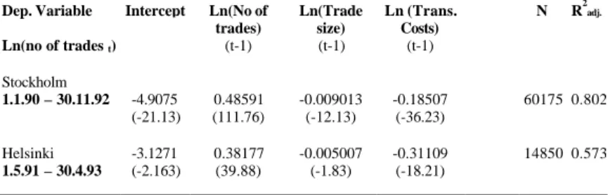
To measure the impact of the STT changes on liquidity the ideal equation would include information on the depth of the order book and measures of the market impact of different sized trades. These measures may not be available for all markets however and certainly not to all participants in the market and we present a publicly available proxy that should measure liquidity better than the commonly used market capitalization or plain volume. In model (17) the liquidity effects are measured as impacts on the dependent variable, the daily number of trades in each stock. The explanatory variables are average daily trade size for the same stock to pick up changes in market size, transaction costs and a set of independent market environment measures such as volatility and interest rates. Since we adjust the dependent variable by trade size the number of trades can be used to measure and compare
trading activity in individual stocks. A lagged impact of the dependent variable number of trades is expected why we also include a lagged dependent variable in the equation. The model is in multiplied form and will thus be evaluated in logarithmic form:
ln(Number of trades t) (17)
= α1+β1ln(Number of trades(t-1)) + β ln(Trade size2 (t-1)) + 3
β ln(Transaction
costs (t-1)) + β ln(Price volatility 4 (t-1)) + β ln(Interest rate 5 (t-1))
In model (18) we replace the transaction cost variables with a STT change dummy that takes the value 0 before the STT change and the value 1 after the STT change. For markets with several changes we use a dummy for each change. We also add dummy variables for devaluation of currency and the changes in foreign ownership legislation that allowed non resident investors to invest freely in the market. This gives an opportunity to compare the impact of these liquidity enhancing structural changes.
ln(Number of trades t )
(18)
= β ln(Number of trades1 (t-1)) + β ln(Trade size2 (t-1)) + 3
β STT change dummy (t-1)
+ β Currency devaluation dummy 4 (t-1) + ?5 Foreign ownership change dummy (t-1)
We also test models (6) and (7) with measures of term-structure changes, international stock-market measures and market impact
1.3.4 Estimating the impact of transaction cost changes on volatility
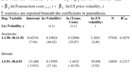
In model (13) we estimate the impact of price volatility on turnover rate. An estimation of the direct effects changes in transaction costs have on volatility is also motivated since one of the arguments for an introduction of STT are that the increased costs of trading would reduce volatility. Equation (19) measures the direct effect of transaction costs on volatility.
ln(Price Volatility t) (19)
= α + 1 β ln(Price Volatility 1 (t-1)) + β ln(Transaction costs2 (t-1)) +β3 ln(US market volatility t )
The price vola tility is measured as difference between highest traded price and lowest traded price on average price and as daily, weekly and monthly variance in returns. The high to low price measure is less sensitive to changes in volume than the variance measure and thus better for our purpose, since there is a relationship between transaction costs and volume. Equation (19) is also tested with the control variables used in equation (13) and (18).
All models are constructed using input variables publicly available at the time of estimation to emphasize the predictive purpose of the models. When variables are considered for inclusion we try to choose variables that generally are used in by market participants for predictive purposes. This approach may reduce the fit of the models to the data but should improve the applicability of the models for actual estimation tasks and ensure that the independent
variables are endogenous. We test the models both with the previous and the same days US return, volume and volatility data since this information is fully exogenous and is used as a proxy for world market data. The US information can be replaced in the models with data from some other major market or world market data. We also estimate the models correcting for possible time trends using the residuals from a regression of the dependent variable against time as the dependent variable.
1.4 The data sample
The data used in this study include detailed daily data from the Swedish stock exchange (Stockholms Fondbörs)1 and all on-market trades and a sample of quotes from the Finnish Stock Exchange (Helsingin Arvopaperipörssi)2. For Sweden the data consists of daily number of traded shares, volume in SEK, number of trades, daily high and low and the closing best bid and ask for the 121 stocks traded during the years 1990, 1991 and 1992. The data is centered on the two dates, January 1 1991 and December 1 1991, when the turn over tax reduction became effective in two steps. When foreign listed stocks and stocks with missing data are excluded the sample is narrowed down to 80 stocks. In addition market aggregate data for all shares traded on the main list over the period (at the end of 1992, 118 companies with several share
1
series) is used for analysis of price impact of the tax change, for liquidity analysis and for market descriptive purposes.
For Finland the data consists of all trades for the 30 stocks that have been traded during the whole period 1991, 1992 and 1993. An overview of the Swedish and Finnish stock market development during the period 1987 to 1998 is provided in table 1. The trade data includes trading price, volume, buying and selling broker dealer as well as information if the trade is made in the limit order book market (downstairs) or in the inter broker dealer market (upstairs). See Booth et al (1998) for a study of the distribution of trades between the upstairs and downstairs markets in Finland.3 The data is centered on May 1, 1992, the date the stamp duty reduction became effective in Finland. In addition a sample of all shares traded on the main list (138 at the end of 1993) is used for analysis of price impact of the tax change, for liquidity analysis and for market descriptive purposes.
The individual stock returns are corrected for dividends and the volume measures are corrected for changes in the number of outstanding stock of the companies. To estimate total market effects we use the all-share stock indexes for Stockholm and Helsinki adjusted for dividends.
To measure the turnover rate we use market capitalization and turnover measures for individual stocks and on a market aggregate basis. We use short- and long-term market interest rates to measure changes in the interest rate level and the term structure. We use market return and turnover data from the New
3
A majority of the larger trades are made in the upstairs market while the price level is determined to a greater extent in the downstairs market.
York stock exchange to proxy world market developments. We use the preceding days measures of the US stock market return and activity since due to the time difference New York opens when the Nordic markets close and most of the effects of New York (and Asia) hit the Nordic markets the following day. We use the Dow Jones Industrial average since this is the index that is used by most participants in the Nordic markets to measure US stock returns on a daily basis. We also compare our findings to estimations using the broader CRSP index for the US market. To measure exchange rate impacts we use the exchange rates of the Swedish krona and the Finnish markka towards the European currency ECU, (now Euro). All variables are measured on a daily level. Note that appendix 2 provides details on recent development of Sweden’s and Finland’s exchanges and the institutional environments.
While the variables in this study make use of intra-day variations (i.e. detailed trade records, bid-ask spread, market impact costs, and so on) all variables are summarized to a single daily observation. As a consequence, for Sweden we end up with 731 trading days over the two years and eleven months period with a total of 58480 observations. For Finland we end up with 500 trading days over the two-year period with a total of 15000 observations.
The primary criterion for inclusion in our sample is that a stock must have a closing bid-ask spread for all days included in the sample. Both the Finnish and Swedish markets characteristically have periods of thinner trade in otherwise liquid stocks. Both
been traded. In the Finnish sample of 30 stocks there is an average of 32 trading days of the 500 days or 6.3 percent, when the stocks have not been traded. This should not be a major problem since all of these stocks have bid ask quotes for all days (except trading halts) and have been traded actively during the later end of the investigated period. In the analysis measures will be taken to adjust for the thinly traded days. Also the thin trading is a natural consequence of high transaction costs and it would be wrong not to include stocks based on this criterion. Most of the days with little or no trading occurs before the changes in STT when some of the trading has migrated to other markets and some trades that may have occurred under lower transaction costs are not executed. We perform comparative studies based on weekly data to ensure that thin trading does not cause erroneous interpretations of our findings. As a result of these exclusions the analysis on company level will be performed on a sample that represents all larger capitalization companies and several smaller companies in Sweden; a total of 61 percent of total market capitalization at the end of the investigated period. The sample of companies used for Finland represents 81 percent of the market capitalization at the end of the investigated period.
2. Empirical findings 2.1 Economic environment
The market was considerably more active after the changes in STT. In the Swedish case there was no other major structural changes in the market around this time. Sweden experienced a currency crisis during the end of 1992 however causing a peak in interest rates and a fall in share prices. The effectively weaker currency may be one reason for the remarkably stronger share prices in 1993. To the extent we include this volatile period
starting about one year after the final STT change we have to be aware of these effects on our findings.
In Finland we can see a substantial increase in turnover when we compare the traded volume during one year before the STT change to traded volume one year after. When we look at a four months period before and after the STT change the turnover of shares does however decrease slightly. One of the reasons for this is that despite an improved environment for securities trading there was other serious problems in the Finnish economy. During the four months after the STT change a severe drop in price levels occurred as a result of a economic policy that was defending a weakening currency with higher interest rates. In this situation a flight of capital offshore is expected. During the autumn 1992 the Finnish markka was devalued and floated which led to a substantial decrease in the exchange rate after the currency crisis settled. This in turn resulted in an increase in the prices and volumes on the stock exchange both due to the adjustment of the exchange to the lower currency and to the improved outlook for the exporting sector, a vital part of the Finnish economy. Also by the beginning of 1993 the restrictions on foreign investments in Finnish securities was lifted. This started a trend towards a situation where close to one half of the most important Finnish companies are owned by investors outside of Finland and this has increased price le vel as well as liquidity and trading volume. In our analysis we attempt to correct for these other environmental changes to isolate the impact of the stamp duty change.
during the late 1980s in most other markets with increases in activity coinciding with market de-regulations and upheavals of market restrictions. In our study we are investigating one of the possible reasons for this increase in turnover the improved liquidity associated with lower costs of transacting. If there is a trend in turnover however this may have an impact on our findings. We estimate comparative results correcting for any trends over time in turnover.
2.2 Predicted effects
Before we examine the actual impact of the STT changes that occur on these markets we predict the expected effects based on our models. The prediction procedure can be divided into four steps. First we determine the effect of the STT change on total transaction costs including brokerage fees and bid ask spreads. When we know the percentual change in STT and when we assume that the change in overall transaction costs have a proportional effect on brokerage fees and bid ask spreads we can calculate expected change in total transaction costs. In Sweden the first STT change of 50 percent was 23 percent of average total transaction costs. The second STT change was 30 percent of total transaction costs. The abolishment of STT in Finland accounted for 20 percent of average total transaction costs. We assume that the brokerage fees and bid-ask spread levels change at least with the same proportion as total transaction costs. This assumption is based on earlier empirical findings but a model for this effect could be developed. Secondly we then expect the total effects on transaction costs including expected changes in brokerage fees and bid ask spreads are 36 and 56 percent for the Swedish STT changes respectively and 37 percent for Finland. Thirdly we estimate the transaction cost elasticity in turnover applying model (13) to daily market data available up to the day
before the STT change, (see tables 3 and 4). We estimate the transaction cost elasticity in prices applying model (16) to aggregated data for the year before the STT change, (see table 6). For Sweden the turnover elasticity estimates are 0.908 and -0.906 while the price elasticity estimates are -0.211 and -0.175. For Finland the turnover elasticity estimate is -1.388 and the price elasticity estimate is -0.177. Finally we use these estimates to calculate the impacts on the current volume, turnover rate and market capitalization to predict the turnover and price level after the STT changes. The effects are calculated with equation (9) and (10) as follows.
Predicted volume = (20)
Current volume * Trans. cost elasticity turnover* Change in Trans. costs STT,BRK,BAS
Predicted market capitalization = (21)
Current capitalization * Trans. cost elasticity price* Change in Trans. costs STT,BRK,BAS
When the turnover and price reactions are estimated using data available the day before the change in STT and equations (20) and (21) we can observe a substantial increase in turnover and a significant increase in prices. For Sweden we predict turnover to increase by 30 percent with the first STT reduction and another 54 percent with the second reduction. The respective increases in the turnover rate are from 18 to 23 percent in the first reduction and a change to 35 percent in the second reduction of STT. For
changes for Sweden are 17.3 percent summed over both STT changes and 6.6 percent for Finland. Compared to the predicted increases in market capitalization the forfeited tax revenue amounts to approximately 2.0 percent for Sweden and 1.6 percent for Finland. When we compare these predictions to actual changes in turnover and prices we find the estimations remarkably accurate, (see table 7). These results are encouraging for the use of our presented estimation technique on other markets. The effects of the changes in transaction costs appear to have a stronger impact on the level of brokerage fees than on the level of the bid ask spread when the estimates are compared to the real outcomes. A more exact model for the total change in transaction costs would improve the accuracy of the predictions.
In all our estimations we consistently use the preceding day’s closing values as input when we estimate the effects on today’s market activity. We are thus taking the position of an investor at the beginning of the day using information available at that moment to make his or her trading decisions. This approach does not affect the significance of the individual coefficients from our regressions, in fact it somewhat improves the t-values. The approach of using lagged values has a negative impact on the R squared measure of the explanatory power of the model. If we use the same day’s values as independent variables the adjusted R squares are in the range of 75 percent for Sweden and 47 percent for Finland, (not reported here). When we use lagged independent variables the adjusted R squares are 56 percent for Sweden and 36 percent for Finland, (see tables 3 and 4). The F values are still highly significant and the t-values for the transaction cost coefficients are 39 for Sweden and 20 for Finland.
2.3 Observed effects on turnover rate and transaction cost elasticity
The sample of 80 Swedish stocks and the 30 Finnish stocks are analyzed using model (13) above. Here we estimate the model using data for the period leading up to the STT changes and data for one year before and one year after the changes. This way we measure the actual impact of an exogenous change in transaction costs and are able to assess the dynamics of the elasticity in transaction cost and asset prices. We are still using lagged values as input variables. The results are presented in tables 3 and 4. The coefficients for the transaction cost are significantly negative on both markets. Rising transaction costs thus have a negative impact on the turnover rate of shares while lower transaction costs have a positive impact on the turnover rate. The long-run transaction cost elasticity settles at slightly higher than or close to one (negative). It is–1.0019 (t-value –39.15) for Sweden and –1.274 (t-value –20.42) for Finland, (see tables 3 and 4).
We also estimate the significance of dummy variables for the STT change, currency crisis followed by the devaluation of the local currency and free foreign ownership of shares. Our results indicate that a significant part of the increase in turnover rate seems to have been caused by the stamp duty change. The devaluation of the currency has a strong impact while the free foreign ownership has a moderate impact on turnover rate. We also achieve consistent results using market aggregate data and all shares indexes as price measures. These findings show that for
(t-value 21.7 and R2 0.77) for Sweden and –1.12 (t-value 10.5 and R2 0.67) for Finland, (not reported here).
A division of the samples from both markets into groups according to capitalization is performed to measure if the sensitivity to changes in transaction costs is larger or smaller in higher capitalization stocks. To the extent that larger capitalization stocks can be considered to be more liquid, we would expect a higher sensitivity since the STT is a larger fraction of the transaction costs and thus the total change in transaction costs due to the tax cut should be larger. There may however be stocks that have a large capitalization and still are traded less than stocks with a lower capitalization due to various company characteristics reflected in a higher bid-ask spread and lower liquidity. A division in portfolios using bid-ask spreads or turnover rate may be a better way to define groups of stock with similar level of liquidity. In table 5 we present the size portfolio results. On the Swedish market during the investigated period the absolute largest capitalization stocks are less sensitive to transaction costs than the large to medium sized companies. Overall the transaction cost elasticity in turnover rate decrease with capitalization as expected. On the Finnish market the highest capitalization stocks are less sensitive to the changes in transaction costs than the medium sized companies. The transaction cost elasticity in turnover rate is the lowest for small capitalization companies in Finland as well. Overall we conclude that higher capitalization is associated with higher transaction cost elasticity in turnover rate. Our findings also indicate that higher trading activity and lower bid-ask spread is associated with higher transaction cost elasticity in turnover rate. These observations are important as they show that each security has a different transaction cost elasticity and that the elasticity for
the whole market cannot be imposed on a single stock or a single group of stocks.
To correct for possible trends in the volume and turnover rate over time we estimate the above equations using the residuals against time to de-trend the series. The adjustment for a possible time trend in the volume and the turnover rate does not change the findings to any significant degree. The estimated coefficients for the transaction elasticity are slightly lower when de-trended turnover measures are used, (not reported).
The estimated coefficients are sufficiently robust. The Durbin-Watson statistic is close to 2 and the Durbin’s h-statistic has a mean close to zero and standard deviation close to one which indicates low autocorrelation in the data used to estimate of the auto-distributed lag model (13). A set of tests for heteroskedasticity in the error term show some signs of heteroskedasticity. When we apply White’s (1980) heteroskedastic -consistent covariance matrix the estimated coefficients are still significant with a slight decrease in t-values, (not reported). When first differences for short-term interest rate and exchange rate are used instead of levels the coefficients are still similar and significant. The transaction cost elasticity increases however since these transformed money market measures have a weaker explanatory power in the model, (not reported).
capitalization is still substantial in proportion to the decrease in revenue for the receivers of transaction costs.
Since the elimination of the STT taxes in Sweden and Finland were results of a lengthy political debate the decisions did not come entirely as a surprise. Still however the decisions can not fully have been incorporated in the prices. The Swedish decision was a part of a larger tax reform and the proposal to the parliament was announced much earlier for both changes. The proposal to change the 2 percent STT in place since 1986 to 1 percent (two-sided) was presented March 29 1990, while the change was introduced January 1 1991. The second change was proposed on October 18 1991, while the change was introduced on the December 1 the same year. In the Swedish cases we are looking at the price reactions both around the date of the proposal and on the introduction date. In Finland the decision was made and implemented fairly quickly with less public discussion than in Sweden. The tax in Finland had been unchanged since 1948 except for a temporary increase during 1985 and 1986. The Finnish decision was made on Tuesday night on April 28 1992 and the change came in force on the May 1 with trading commencing on May 4. The price reaction thus should have occurred from April 29 onwards. The consolidated numbers including earlier STT changes are presented in table 4. The average changes in the price level is measured as the change in the last trade (logarithmic daily returns) around the date when the proposals to change the STT law was presented and around the date when they where introduced separately. In Sweden the price impact of the two announcements is 0.38 and 2.47 percent for the 121 most liquid
stocks and -0.46 and 2.56 percent for the market index4. The reaction to the second proposal to abolish the STT completely is stronger than the reaction to the initial reduction. The price development is negative during the introduction dates in Sweden. The introduction of the STT change is no surprise, since the decision was finalized much earlier. In Finland the price effect including announcement and introduction was 6.2 percent for the 30 most liquid stocks and 5.51 percent for the market index5 in Finland. The Finnish case is more clear-cut since the tax has been established for a long time and it was cut to improve the functioning of the market. Also the announcement and introduction occur over a few days which makes the study of the price effects more reliable. See table 6 for an overview of the STT changes and the price effects.
2.5 Test of the impact on prices
The effects of the STT changes may not be fully incorporated into prices until the improvement in liquidity have been fully adjusted for in the terms of market activity. That is why we also estimate price change to the point when the turnover of shares has reached the estimated level. For Sweden the estimated level of turnover is reached 14 and a half months after the second change in STT. For Finland the estimated level of turnover is reached just under 8 months after the change in STT. The market capitalization for the whole Swedish market at the point when the estimated yearly volume is reached the increase is 13.9 percent compared to the
level before the change in STT. This is however 0.5 percent less than the return on the interest rate market of 14.4 during the same period. For Finland the increase in market capitalization for the whole market is 8.6 percent compared to the level before the change in STT. This is 0.8 percent less than the return on the interest rate market of 8.89 percent for the same period. The extremely high interest rate level during this period should be replaced with a long term average when we look at the long-term effects. The investors may have discounted some of the lower interest rate levels to come when they determined the prices for common stock. (The short term market interest rates have stabilized around four percent on both markets during 1997-2000). When we look at the raw changes in market capitalization during the period after the STT changes they are close to the estimated price increases when we consider that both markets have several disturbing events during or close to the investigated periods. Note that the change in STT in Sweden was two times larger than the change in Finland and that it appears to take twice the time for the Swedish market to adjust to the lower transaction costs. The observations in this section are only stated as an example of our hypothesis of a relationship between turnover activity and asset prices and have no statistical validity.
We attempt a test of the validity of our proposal that the price changes over the period when the turnover is adjusting to new transaction cost levels can (at least partly) be attributed to the changes in transaction costs. First we estimate how much of the price changes during the first month after the STT change for our sample of companies from Sweden and Finland can be explained by changes in transaction costs. Secondly we estimate how much of the price changes over the period when the turnover is adjusting to new transaction cost levels can be explained by changes in transaction costs. This period is 14.5 months for
Sweden and 8 months for Finland. We apply equation (15) from section 3 to estimate the relation between the excess return and the change in transaction cost and include as control variable for size the average market capitalization and as control variable for liquidity the turnover rate during the predicted adjustment period t-1 to t. Other control variables measuring the market environment during the period cannot be inclued in this estimation due to a low number of data points why we estimate a simpel version of equation (15) in equation (22) below.
= α1+β1x((c t - c t-1) / c t-1) + β Mean Market Cap + 2x
+β3xτt−>t−1 (22)
The findings are presented in tables 8a and 8b. For the Swedish sample of 80 stocks the relation change in transaction costs to the excess return is significant both for the one month period and the 14.5 month periods after the STT change. When the change in turnover rate or alternatively the total turnover rate during the period after the STT change is added to the equation this factor explains excess returns better than the change in transaction costs for the shorter period, (see table 8a). The estimations on the Swedish data indicates that the lower transaction costs cause higher turnover rates and an expected increase in prices due to a lower demand for compensation for illiquidity. The adjusted R squares are between 4.7 percent for the first month after the STT change and between 6and 8 percent for the longer adjustment period. For the sample of 30 Finnish companies none of the variables are significant, (see table 8b).
in line with our estimated price changes for both markets supporting the applicability of the presented models. When the returns in excess of the risk free market interest are considered the returns are much lower than the predicted returns and the similarities between predicted and raw price changes have to be considered as a strike of luck.
2.6 Observed liquidity effects and the impact of other structural changes
The sample of 80 Swedish and the 30 Finnish stocks during the STT change periods are analyzed using model (17) and (18). The findings are reported in table 9.
For both markets the liquidity measured as the number of trades scaled by trade size has improved significantly after the STT changes. In Sweden the total abolishment had a larger impact on trading activity than the earlier cut of equal size. In the case of Finland in addition to the STT change a large part of the increase in trading activity is due to the two other major structural changes, devaluation and free foreign ownership of securities. The effects of the currency devaluation appear to be assimilated by the market during the weeks around the devaluation. A dummy variable that gives a different intercept to 18 days around the devaluation picks up most of the effect. The change to free foreign ownership of shares has more long-term effects and is one of the major factors in sustaining the growth in the Finnish market. The effect of the change to free foreign ownership of shares appears to have little impact during the investigated period with positive price and turnover effects picked up by the dummy variable during three days after the change of January 1993.
2.7 Observed volatility effects
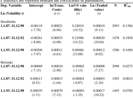
In the regressions presented in table 3 the volatility coefficient measured as the difference between high and low price to average price, takes a significantly negative value when it is regressed against turnover rate. This indicates that the higher turnover associated with lower transaction costs also can be associated with lower volatility. This is confirmed by the regressions of volatility against transaction costs using equation (19) and reported in table 10. The long term transaction cost elasticity in high low dispersion takes a significantly positive value at 0.40, (long-term coefficient derived from short-term and lagged transaction cost variable). The Finnish case give an indication of increasing volatility with higher turnover around the STT change, that we interpret as a result of the extreme volatility on the downside during end of 1992. A more detailed study of 1992 with regards to volatility is suggested for future research. In table 11 aggregate market data is analyzed over a longer time period and a positive relationship between transaction costs and volatility is documented for both markets. In these estimations the volatility is measured as the weekly variance in logarithmic returns, US market volatility is included to measure international volatility changes and traded value is included to pick up the relationship volume to volatility. The argument that higher transaction costs would decrease volatility is as follows not supported by our findings. Particularly in the Swedish case lower transaction costs appear to have a decreasing effect on volatility in securities prices.
2.8 Comparison to other markets where the STT has been changed
The case of Sweden’s STT reductions can be compared to Australia where a similar halving of stamp duty on securities trading have taken place and a total abolishment of the tax may be considered. The halving of the STT in Sweden increased turnover by 30 percent and prices by 7.5 percent. An improvement of social welfare net revenue losses of 14 billion SEK (1.7 billion US) can be associated with the STT change. In Australia the turnover of shares increased after the halving of the stamp duty by 26.2 percent, the price reaction to the announcement was 1.73 percent and a net 4.6 billion AUD (2.9 billion US) increase in social welfare can be associated with the tax change. The Swedish tax was initially higher at 2 percent compared to 0.6 percent for Australia. Thus the loss in tax revenue was substantially higher in Sweden. Since the tax in Sweden was left at one percent in the first change the following increase in capitalization was also lower. Correcting for these differences the increase in capitalization of about 20 times the forfeited tax revenue in Sweden and about 40 times the forfeited tax revenue in Australia are very much in line. The total abolishment of a tax on securities trading in Sweden in December 1991 is followed by a substantial increase in turnover and prices. The full effect is reached 14 months after the abolishment of tax with the increase in capitalization net revenue loss of 70 billion SEK (8.5 billion US). The current position of Stockholm as one of the leading European exchanges with a yearly turnover at the same level as and larger capitalization than AMEX in the US would not have been reached with a one percent STT tax on trading.
Since the level of tax in Australia is one third of what the le vel of tax was in Sweden we may not expect as drastic changes in
turnover and capitalization if the tax was to be lowered or abolished in Australia. On the other hand today’s market are more efficient and liquid than they were in 1991 and 1992 when the Swedish STT changes took effect. We have in this paper showed that decreased transaction costs have a larger impact on the turnover in more liquid stocks (with high capitalization) and earlier studies have also found a higher sensitivity to transaction cost changes on more liquid markets.
The case of Finland’s stamp duty reduction can be compared to New Zealand and Singapore where the stamp duty on securities trading has been abolished. In preliminary findings from Singapore we detect an increase in the turnover of shares after the STT abolishment in early 1997. A more detailed study of Singapore is required to draw any conclusions from this.
3. Conclusions and Research Agenda
We set out to apply a model that can accurately predict and measure the effects STT changes have on the turnover rate and asset prices. We specify a model that predicts changes in turnover rate and asset prices that are close to the observed effects. We conclude that STT changes have a significant impact on the price levels and the trading activity in Sweden and Finland. The price reactions to the announcements of STT adjustments downwards are positive. The transaction cost elasticity in asset prices is estimated to be between -0.12 and -0.21 for Sweden and between –0.18 and –0.33 for Finland. The estimations of the effects on turnover rate show significantly negative coefficients for
brokerage fees and bid ask spreads have rapidly followed the change in STT in the expected proportion.
Transaction costs have remained on a higher level in Finland than in Sweden. The transaction cost elasticity levels as well remain higher in Finland after the STT changes, partly due to the smaller more concentrated market and partly because the brokerage fees have not been as flexible as in Sweden. This is an indication that there is further means of increasing the efficiency of the Finnish stock market through lower costs. A more flexible and public brokerage fee policy in Finland would have a significant impact on the liquidity and as a result the size of the market.
Some of the improvements in market liquidity of the Nordic markets can be attributed to an international increase in stock market activity. Internal changes in exchange rate policy and the liberalization of foreign ownership of shares in Nordic companies have a large impact on the activity of the local stock markets as well. After controlling for these effects we still find that the abolishment of STT is an important factor explaining the increase in activity on these markets. Our findings indicate that in other markets an introduction of a STT can be expected to decrease demand for trading, have a negative effect on turnover with an elasticity of -1 or higher in absolute magnitude, to decrease liquidity and thus to have a negative impact on asset prices. A decrease in STT on the other hand can be expected to compensate for the loss in tax revenue by an increase in liquidity and asset prices that improve the total social welfare by more than the loss of revenue. We find it reasonable to propose that the remarkable increases in volume, liquidity and prices the Swedish and Finnish stock markets have experienced since 1993 would not have been possible if the security transaction taxes had been
retained. These findings also emphasize that transaction taxes may have negative effects other markets such as real estate. Further analysis of the price effects of transaction costs can be carried out in the capital asset pricing framework. The effects of transaction cost changes on the premium demanded on less liquid assets such as stocks compared to the premium demanded on more liquid assets such as bonds can be evaluated. A new approach is needed particularly since in this paper we show empirically that the long run transaction cost elasticity in turnover for two Nordic markets is greater than one in absolute value. We find that traditional theory cannot explain asset prices correctly and a more dynamic asset-pricing model incorporating endogenous trading is needed.