Optimal Filtering and Magnetometer-free Sensor Fusion: Applications to Human Motion Inertial Sensing

(1)

Ph.D Course in Information Engineering

Optimal Filtering and Magnetometer-free

Sensor Fusion: Applications to Human

Motion Inertial Sensing

Candidate:

Stefano Cardarelli

Advisor:

Prof. Sandro Fioretti

Coadvisor:

Ing. Federica Verdini Ing. Alessandro Mengarelli

(2)

(3)

Ph.D Course in Information Engineering

Optimal Filtering and Magnetometer-free

Sensor Fusion: Applications to Human

Motion Inertial Sensing

Candidate:

Stefano Cardarelli

Advisor:

Prof. Sandro Fioretti

Coadvisor:

Ing. Federica Verdini Ing. Alessandro Mengarelli

(4)

Facoltà di Ingegneria

Ph.D Course in Information Engineering Via Brecce Bianche – 60131 Ancona (AN), Italy

(5)

(6)

(7)

Abstract

During the last decade, the use of inertial sensors in human motion analysis has occupied a central role in the biomedical and electronic engineering scientific literature. The portability and relative low cost of such equipment opened up to a number of domestic, clynical, research and rehabilitation scenarios, leading to a growing interest in software methodologies to obtain accurate data from inertial and magnetic information. In the present dissertation a thorough study is reported regarding a series of common application of inertial sensors in human motion analysis, considering purely inertial measurements. Regardless of the complexity of the techniques that may be involved in the compensation of magnetic distorsions, the present work aims to investigate and assess the accuracy limits of purely inertial setups, in order to give an estimate of the reliability of such kind of minimal setup when other information sources are obstacled for relatively long epochs of time (if not for the whole duration of the measurement session). The present experimental studies concern a comparative study on Extended and Unscented Kalman filtering for sensor fusion in displacement and orientation estimation of human center of mass (CoM) during treadmill walking, center of pressure (CoP) and lower body joint angles estimation during unperturbed posture, pedestrian dead reckoning. A custom calibration method for navigation and local reference frames alignment in magnetometer-free setups is also reported. Results present accuracies within 2 deg (orientation) and 1.5 mm (displacement) for CoM and lower body joints angles estimations, high correlation between estimated and measured CoP, predictability in dead reckoning error drift and improvement in 90 deg turns estimation accuracy using a custom methodology.

(8)

(9)

Chapter 1 Introduction

Position and attitude tracking of physical bodies in space is of common interest in several engineering and research contexts. From aerospace, naval and automobilistic guidance systems [1], to virtual reality, robotics and human motion tracking for clinical and sports applications, the deterimination of such quantities is at the very basis of systems control and analysis of motion patterns in support of diagnostics and rehabilitation programs [2]. The variety of existing sensors for both attitude and position estimation, reflects their wide range of application contexts. Also, the costs and the volume of the employed hardware is strictly dependent from a series of factors including: required accuracy levels, minimal system portability, outdoor/indoor applications, budget limits, etc.. Furthermore, the physical principle the tracking system is based on, critically influences the application context and expected accuracy. As an example, Global Positioning Systems (GPS) rely on a time information to be elaborated by the target device, so that body triangulation can be achieved by the integration of signals coming from multiple satellites: hence the tracking accuracy is strictly dependent on satellites coverage and weather conditions, and it is obviously restricted to outdoor usage. Environmental and geographical information blockage in tracking systems is commonly referred to as shadowing.

The partial or total lack of information for relatively long or short epochs of time in real time tracking applications, is usually dealt with an increased number of sensors whenever it is possible to assume that the lack of information from one sensor can be compensated by the availability of the others. This implies using sensors clusters with different operating physical principles or arrangements in the measurement environment. Merging information from an array of sensors to obtain an estimate of a certain physical quantity (e.g. position and/or orientation of a body in space) is called sensor fusion. Sensor fusion tipically involves a filtering process to obtain estimates of the desired quantity.

The word filtering has assumed two main meanings throughout the years. At first, the concept of filtering was strictly connected to the use of analog circuits with frequency selective behaviors, or tuned circuits, to block unwanted systems behaviors in the frequency domain. One of the most important examples of this kind of filtering paradigm in the field of electrical engineering can be ascribed to the wave trap for transmission lines1_{. Henceforth, tuned filters,}

and consequently filter design theory, became more complex in order to satisfy amplitude and phase response requirements for a wide range of applications including digital filtering (e.g. Butterworth and Chebyshev filters [3]). In the 1940-50 decade, the work of Wiener and Kolmogorov [4, 5] introduced to the concept of statistic filtering, where the separation of wanted and unwanted components of a signal (i.e. noise) was performed on the basis of their stationary statistical properties. However, this stationarity assumption badly coped with

1_{A line wave trap example:} _{http://www.steel-sa.com/bzzz/wp-content/uploads/2011/06/ARTECHE_CT_}

(12)

applications where nonstationary processes or noises were involved. For this reason, in the early 1960s the work of Kalman and Bucy [6,7] introduced a new filtering technique, which did not required the stationarity assumption of the Weiner and Kolmogorov approaches. This particular technique soon assumed the name of Kalman filtering.

In this dissertation the term filtering is always referred to its statistical significance. Henceforth, given a system (stationary or nonstationary) in its discrete-time state-space form, the concept of filtering in the Kalman conception can be summarized in the minimum-square error estimation of the state at the discrete time-frame k, given a number l = k of available observations. At the same time, for l < k the same problem is referred to as prediction, and for l > k is referred to as smoothing [8–10].

Kalman filtering was a breakthrough in the field of information filters and sensor fusion. Due to its state-space formulation, it allowed great generalization with respect to the process model and the observation (measurement) process model involved, so that once the estimation problem is defined in its state-space form, it is possible to iterate the same algorithm for any application context. Also, the compact form of the algorithm allowed relatively easily-feasible solutions (and readaptations, in particular regarding nonlinear and nonstationary processes and observation functions) from a implementative point of view, both in terms of software and hardware2_{. Furthermore, thanks to its versatility, Kalman filtering theory very well suits}

the aforementioned problem of sensor fusion: indeed, such applications simply involve the use of sensor readings into the state propagation model in addition to the array of sensors readings injected through the measurement process.

As introduced above, the shadowing problem can be compensated through a sensor fusion software/hardware setup. Fortunately, the use of inertial sensors for orientation and position estimation overcomes this issue, being immune to shadowing. Indeed, orientation and position can be ideally estimated through the integration of, respectively, gyroscope and gravity-free accelerometer information. Nevertheless, direct integration of noisy signals eventually leads to unbounded drift, so that an accurate estimate can be expected for very short periods of time (dependently on sensors accuracy and superimposed noise). As a matter of facts, orientation estimation must be bounded in a sensor fusion process, including accelerometer gravitational readings in the measurement process to mitigate the drifting behavior induced by the integration of the gyroscope information during the state propagation [1, 11–14]. Magnetometer measurements as well are usually integrated in magnetic-inertial sensors setups to improve estimation accuracy. On the other hand, concerning position estimation through inertial sensing, unless direct observations are added to the position propagation via gravity-free acceleration integration [15], there is no way to avoid estimation drift without resorting to zero velocity update methods [16–20]. Such kind of techniques involve the injection of a pseudo "zero-velocity-measurement" into the measurement process whenever the inertial sensor is considered to be still. In pedestrian dead-reckoning systems the foot stance phase, during normal walking, is usually identified and leveraged for this purpose.

In the last two decades, inertial-magnetic sensing, in combination with Kalman filtering or similar "complementary" techniques (e.g. heuristic optimization-based measurements integrations like [21]), became quite popular in the field of human motion analysis, due to the extremely high portability and low costs of inertial systems with respect to gold-standard optical tracking systems (i.e. stereophotogrammetry). Several works can be found in literature regarding a wide range of clinical, tracking and monitoring related applications:

2_NASA _technical _memorandum: _{https://ntrs.nasa.gov/archive/nasa/casi.ntrs.nasa.gov/}

(13)

dead-reckoning [17, 18,20, 28–30], posture analysis [31], APA and freezing recognition in Parkinson patients [32–34] and other medical related instances [35].

In recent times, a common interest among inertial measurement units application studies has arised, regarding the problem of magnetometer-related disturbances. While accelerometer gravitational data is included in the measurement process when the linear acceleration is considered to be null, i.e. body stationarity, the hypothesis made to include magnetometer readings is related to the assumption of earth magnetic field sensing only and in general on the assumption of homogeneous magnetic fields [36,37]. As a consequence, many studies make efforts to model and estimate magnetic distances in order to remove them from readings [38–40].

In the present dissertation a thorough study is reported regarding a series of common appli-cation of inertial sensors in human motion analysis considering purely inertial measurements. Regardless of the complexity of the techniques that may be involved in the compensation of magnetic distorsions, the present work aims to investigate and assess the accuracy limits of purely inertial setups, in order to give an estimate of the reliability of such kind of minimal setup when other information sources are obstacled for relatively long epochs of time (if not for the whole duration of the measurement session).

The present work is divided as follows: Chapter 2provides an introduction to random variables and probability theory, with a particular attention on the orthogonality principle, which is the basis for the optimal estimator as reported by Kalman in its first formulation [6]. The essential aim of this chapter is to define the strong connection between the field of probability theory and the concept of least-mean-square estimators thanks to the geometrical properties of the Hilbert spaces of random variables. Indeed, it is possible to observe, since the first few sections, that the very definition of Bayes’ Theorem constitutes the bone structure of the a posteriori estimator without the optimality asset, which is allowed by certain characteristic of the processes involved. Also, it is possible to demonstrate that the Bayesian recursive estimator is a particular case of univariate linear Kalman filter3_{. Chapter}

3introduces the concept of stochastic processes and hence the properties of Markov processes to finally allow the definition of the linear Kalman filter and its well-known nonlinear variants, the Extended Kalman filter (EKF) and the Unscented Kalman filter (UKF). Pseudocode is available for each of the aforementioned formulations in the relative sections, and it matches the actual implementation employed in the following chapter. Chapter 4reports the quaternion-state EKF proposed by Sabatini in 2006 [13] alongside with its adaptation to the lack of magnetometer information and the Unscented transform. A custom-made calibration procedure is also presented to allow to refer inertial data to an earth-fixed navigation frame without the earth magnetic north information (transversal plane). The aforementioned calibration procedure, alongside with the magnetometer-free adaptation of the quaternion-state KF, played a key role in every experimental application presented in this manuscript. Finally a series of studies is reported regarding magnetometer-free approaches to human motion analysis, including center of mass displacement and pelvis orientation estimation during treadmill walking, center of pressure model-aided estimation during unperturbed balance mantainment, pedestrian dead-reckoning and lower body joints angles estimation during perturbed posturography. Each section reports relative state of the art and introductory subsection, results and discussions. Finally, a summary discussion of the whole manuscript is reported in chapter5.

(14)

(15)

Bibliography

[1] Malcolm David Shuster. A simple kalman filter and smoother for spacecraft attitude.

Journal of the Astronautical Sciences, 37(1):89–106, 1989.

[2] Akin Avci, Stephan Bosch, Mihai Marin-Perianu, Raluca Marin-Perianu, and Paul Havinga. Activity recognition using inertial sensing for healthcare, wellbeing and sports applications: A survey. In 23th International conference on architecture of computing

systems 2010, pages 1–10. VDE, 2010.

[3] James Edward Storer. Passive network synthesis. McGraw-Hill, 1957.

[4] Norbert Wiener. Extrapolation, interpolation, and smoothing of stationary time series:

with engineering applications. MIT Press, 1950.

[5] A No Kolmogorov. Interpolation and extrapolation of stationary stochastic sequences.

Izv. AN SSSR, Matematika, 5, 1941.

[6] Rudolph Emil Kalman. A new approach to linear filtering and prediction problems.

Journal of basic Engineering, 82(1):35–45, 1960.

[7] Rudolph E Kalman and Richard S Bucy. New results in linear filtering and prediction theory. Journal of basic engineering, 83(1):95–108, 1961.

[8] Brian DO Anderson and John B Moore. Optimal filtering. Courier Corporation, 2012. [9] Simon Haykin. Kalman filtering and neural networks, volume 47. John Wiley & Sons,

2004.

[10] Arthur Gelb. Applied optimal estimation. MIT press, 1974.

[11] MD Shuster and S Oh. Three-axis attitude determination from vector observations.

Journal of Guidance, Control, and Dynamics, 4(1):70–77, 1981.

[12] Daniel Choukroun, Itzhack Y Bar-Itzhack, and Yaakov Oshman. Novel quaternion kalman filter. IEEE Transactions on Aerospace and Electronic Systems, 42(1):174–190, 2006.

[13] Angelo M Sabatini. Quaternion-based extended kalman filter for determining orientation by inertial and magnetic sensing. IEEE Transactions on Biomedical Engineering,

53(7):1346–1356, 2006.

[14] IY Bar-Itzhack and Yaakov Oshman. Attitude determination from vector observations: Quaternion estimation. IEEE Transactions on Aerospace and Electronic Systems,

(1):128–136, 1985.

[15] Nima Enayati, Elena De Momi, and Giancarlo Ferrigno. A quaternion-based unscented kalman filter for robust optical/inertial motion tracking in computer-assisted surgery.

(16)

[16] Eric Foxlin. Inertial head-tracker sensor fusion by a complementary separate-bias kalman filter. In Proceedings of the IEEE 1996 Virtual Reality Annual International Symposium, pages 185–194. IEEE, 1996.

[17] Eric Foxlin. Pedestrian tracking with shoe-mounted inertial sensors. IEEE Computer

graphics and applications, (6):38–46, 2005.

[18] Xiaoping Yun, Eric R Bachmann, Hyatt Moore, and James Calusdian. Self-contained position tracking of human movement using small inertial/magnetic sensor modules. In

Robotics and Automation, 2007 IEEE International Conference on, pages 2526–2533.

IEEE, 2007.

[19] Xiaoping Yun, Eric R Bachmann, and Robert B McGhee. A simplified quaternion-based algorithm for orientation estimation from earth gravity and magnetic field measurements. Technical report, Naval Postgraduate School Monterey Ca Dept of Electrical and Computer . . . , 2008.

[20] Shu-Di Bao, Xiao-Li Meng, Wendong Xiao, and Zhi-Qiang Zhang. Fusion of iner-tial/magnetic sensor measurements and map information for pedestrian tracking. Sensors, 17(2):340, 2017.

[21] Sebastian OH Madgwick, Andrew JL Harrison, and Ravi Vaidyanathan. Estimation of imu and marg orientation using a gradient descent algorithm. In Rehabilitation Robotics

(ICORR), 2011 IEEE International Conference on, pages 1–7. IEEE, 2011.

[22] Thomas Seel, Jörg Raisch, and Thomas Schauer. Imu-based joint angle measurement for gait analysis. Sensors, 14(4):6891–6909, 2014.

[23] Elena M Gutierrez-Farewik, Åsa Bartonek, and Helena Saraste. Comparison and evaluation of two common methods to measure center of mass displacement in three dimensions during gait. Human movement science, 25(2):238–256, 2006.

[24] Marianne J Floor-Westerdijk, H Martin Schepers, Peter H Veltink, Edwin HF van Asseldonk, and Jaap H Buurke. Use of inertial sensors for ambulatory assessment of center-of-mass displacements during walking. IEEE transactions on biomedical engineering, 59(7):2080–2084, 2012.

[25] H Martin Schepers, Edwin HF Van Asseldonk, Jaap H Buurke, and Peter H Veltink. Am-bulatory estimation of center of mass displacement during walking. IEEE Transactions

on Biomedical Engineering, 56(4):1189–1195, 2009.

[26] Bora Jeong, Chang-Yong Ko, Yunhee Chang, Jeicheong Ryu, and Gyoosuk Kim. Com-parison of segmental analysis and sacral marker methods for determining the center of mass during level and slope walking. Gait & posture, 62:333–341, 2018.

[27] Patrick Esser, Helen Dawes, Johnny Collett, and Ken Howells. Imu: inertial sensing of vertical com movement. Journal of biomechanics, 42(10):1578–1581, 2009.

[28] Antonio Ramón Jiménez, Fernando Seco, José Carlos Prieto, and Jorge Guevara. Indoor pedestrian navigation using an ins/ekf framework for yaw drift reduction and a foot-mounted imu. In 2010 7th Workshop on Positioning, Navigation and Communication, pages 135–143. IEEE, 2010.

(17)

[29] Stéphane Beauregard. A helmet-mounted pedestrian dead reckoning system. In 3rd

International Forum on Applied Wearable Computing 2006, pages 1–11. VDE, 2006.

[30] Pragun Goyal, Vinay J Ribeiro, Huzur Saran, and Anshul Kumar. Strap-down pedestrian dead-reckoning system. In 2011 international conference on indoor positioning and

indoor navigation, pages 1–7. IEEE, 2011.

[31] Miguel F Gago, Vitor Fernandes, Jaime Ferreira, Hélder Silva, Luís Rocha, Estela Bicho, and Nuno Sousa. Postural stability analysis with inertial measurement units in alzheimer’s disease. Dementia and geriatric cognitive disorders extra, 4(1):22–30, 2014. [32] Benoît Sijobert, Jennifer Denys, Christine Azevedo Coste, and Christian Geny. Imu

based detection of freezing of gait and festination in parkinson’s disease. In 2014 IEEE

19th International Functional Electrical Stimulation Society Annual Conference (IFESS),

pages 1–3. IEEE, 2014.

[33] Martina Mancini, Lorenzo Chiari, Lars Holmstrom, Arash Salarian, and Fay B Horak. Validity and reliability of an imu-based method to detect apas prior to gait initiation.

Gait & posture, 43:125–131, 2016.

[34] Christine Azevedo Coste, Benoît Sijobert, Roger Pissard-Gibollet, Maud Pasquier, Bernard Espiau, and Christian Geny. Detection of freezing of gait in parkinson disease: preliminary results. Sensors, 14(4):6819–6827, 2014.

[35] Xuzhong Yan, Heng Li, Angus R Li, and Hong Zhang. Wearable imu-based real-time motion warning system for construction workers’ musculoskeletal disorders prevention.

Automation in Construction, 74:2–11, 2017.

[36] WHK De Vries, HEJ Veeger, CTM Baten, and FCT Van Der Helm. Magnetic distortion in motion labs, implications for validating inertial magnetic sensors. Gait & posture, 29(4):535–541, 2009.

[37] Wolfgang Teufl, Markus Miezal, Bertram Taetz, Michael Fröhlich, and Gabriele Bleser. Validity, test-retest reliability and long-term stability of magnetometer free inertial sensor based 3d joint kinematics. Sensors, 18(7):1980, 2018.

[38] Gabriele Ligorio and Angelo Sabatini. Dealing with magnetic disturbances in human motion capture: A survey of techniques. Micromachines, 7(3):43, 2016.

[39] Bingfei Fan, Qingguo Li, and Tao Liu. How magnetic disturbance influences the attitude and heading in magnetic and inertial sensor-based orientation estimation. Sensors, 18(1):76, 2018.

[40] Daniel Roetenberg, Henk J Luinge, Chris TM Baten, and Peter H Veltink. Compensation of magnetic disturbances improves inertial and magnetic sensing of human body seg-ment orientation. IEEE Transactions on neural systems and rehabilitation engineering, 13(3):395–405, 2005.

(18)

(19)

Chapter 2 Probability, Random Variables and

Optimal Estimators

This first chapter will cover the basis of probability theory. In order to fully comprehend all the aspects of the filtering problem, and finally to appreciate the proposed solutions, it is necessary for the reader to have a good grasp on the mathematical aspects of the axiomatic definition of probability and its geometrical interpretation.

Any filtering problem can be defined as the matter of knowing as closely as possible the true state of a (dynamic) system of which the measurements (observations) are available. Indeed, the statement "as closely as possible" in terms of technical and engineering purposes should be replaced with "short of a small, known error". In the following chapters this will be proven feasible, and also the state estimation will be proven optimal in a least-mean-square sense. Further on, all states estimations of a given system and its relative measurements (observations), will be defined in terms of stochastic processes. Hence, the necessity to define the concepts of probability spaces and random variables as mathematical tools to build good (or optimal) observers for the given problem.

2.1 Set theory, axioms of probability, and probability spaces

2.1.1 Set theory

Let us define a set A as a collection of items, such as colours, numbers, experimental outcomes etc.; those items can be defined as elements ξ of the set so that:

A = {ξ1, ξ2, . . . , ξn}; ⇐⇒ ξi∈ A ∀i = 1, 2, . . . n (2.1)

All the sets that we consider in this dissertation are subsets of a universe set defined as S.

A ⊆ S (2.2)

Example 1. Considering S as the real numbers axis, then A = N is a subset of S.

Considering the definition of universe set, it is possible to define also the null or empty set

A = {} or A = 0 (2.3)

(20)

Inclusion: we have already seen the inclusion operator in (2.2), so that if every element of a set B are contained in A, then

B ⊂ A ⇐⇒ B = {ξ1, ξ2, . . . , ξn} with ξi∈ A, ∀i = 1, 2, . . . , n (2.4)

Sum or Union and Difference: It is possible to define the sum or union operator, so

that the set

A + B (2.5)

contains all the elements of A or of B or of both. It also is easy to see that

A + B = B + A (2.6)

(A + B) + C = A + (B + C) = A + B + C (2.7)

A + A = A (2.8)

Similarly, the difference

A − B (2.9)

is a set that consists of elements of A that are not in B.

Product or Intersection: The product or intersection of two sets can be defined as

AB (2.10)

and it is a set that consists of elements that are common to both sets. It is trivial to see that

AB = BA (2.11)

(AB)C = A(BC) = ABC (2.12)

AA = A (2.13)

If two sets have AB = 0 they are said mutually exclusive.

Complement: Finally, the complement of a set can be defined as

A = S − A (2.14)

which is the set of elements that do not belong to A.

With those definitions it comes natural to see that the null and S sets have the following properties:

(21)

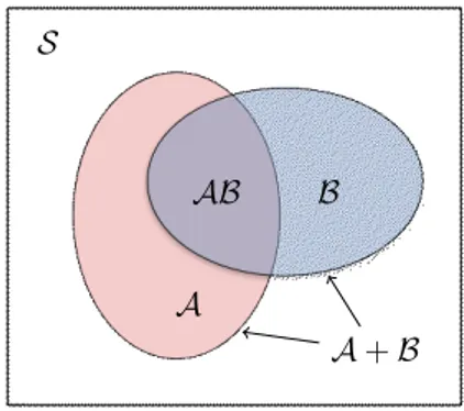
• A + 0 = A; A − 0 = A; A0 = 0 • A + S = S; A − S = 0; AS = A • S = 0 • A + A = S • AA = 0 S A B AB A + B

Figure 2.1: Venn diagram representation of the union and intersection operators.

2.1.2 Axioms of probability

Now that all the fundamental properties of sets have been laid out, it is useful for further dicussion to define a class of sets called a field (F).

Definition 1 (Field). A field is a non-empty class of sets that has the following properties :

• if A ∈ F then A ∈ F.

• if A ∈ F and B ∈ F then A + B ∈ F, AB ∈ F and A − B ∈ F.

Furthermore, if the sets A1, A2, . . . An belong to F, and also the sets • {A1+ A2+ · · · + An} ∈ F

• {A1A2. . . An} ∈ F

then the field F is called a Borel Field.

Thanks to this last definition, we have obtained a mathematical object in which sets and operations between sets are still contained in the same environment and share some useful properties.

Let us now identify the elements ξ of S as experimental outcomes. Hence, defining intuitively an experiment as a set of possible outcomes which consitute a set S, it is possible to state that any subset A ⊂ S as an event. Also, the null and S sets in this context, assume the respective properties of impossible and certain events.

Example 2. Let us define our experiment as the cast of a six-faced die: then S =

{1, 2, 3, 4, 5, 6}. Hence, the subset of even numbers A = {2, 4, 6} is a possible event of

our experiment.

From the example above, it is possible to notice that the event A has a certain probability to happen if the die is cast. The concept of probability of an event P (A) can be also defined as a mathematical object which has certain properties called the axioms of probability:

• P (A) ≥ 0 • P (S) = 1

(22)

• P (A + B) = P (A) + P (B) − P (AB) with the following corollaries:

• P (0) = 0

• P (A) = 1 − P (A) ≤ 1

• P (A + B) = P (A) + P (B) if the events are mutually exclusive. Finally, we can formally define the concept of experiment:

Definition 2 (Experiment). An experiment E is the following:

• A set S of elements (outcomes) ξ and it is the certain event. • A Borel Field consisting of subsets of S called events.

• A number P (A) assigned to every A which satisfies the axioms of probability.

Hence, it is possible to write the experiment as something that is specified by E : (S, F, P )

Probability on the Real Line

The definition of experiment makes it possible to construct a probability space. An important example of such kind of space is the Real Line. The importance of covering this aspect lies in the notation used to define such probability space. This will become clearer when the concept random variable is introduced in section 2.3.

On the real line probability space, the outcomes of an experiment are real numbers. Sums and products of events are still on the same probability space, making it suitable as a Borel

Field. It is common to assume the positive part of the real line as the a time line, so that

S = R and t ∈ S. Assuming an integrable function of time as

α(t) ≥ 0

Z ∞

0

α(t)dt = 1 (2.15)

we say that the probability of an event to happen from time t1 to an arbitrary time t2 is

P {t1≤ t ≤ t1} =

Z t2

t1

α(t)dt (2.16)

this is defined as a random call. Notice that the property of the real line alongside with the form of (2.15) and (2.16) are compliant with the definition of experiment.

2.2 Conditional probability, total probability, Bayes’ theorem

and independent events

2.2.1 Conditional probability

In an experiment E : (S, F, P ) let us assume a non-impossible event M ⊂ S so that

(23)

we define the Conditional Probability as the "probability of an event A ⊂ S to happen

assuming M" as

P (A|M) = P (AM)

P (M) (2.18)

The probability P (A|M) is obviously zero if the two events are mutually exclusive. Also if M ⊂ A then P (A|M) = 1. Finally, it is possible to prove that from the experiment E : (S, F, P (A)) it is possible to create a new experiment E1: (∗, ∗, P (A|M)) which outcomes

form the same universe and events form the same Borel Field, but has different probabilities.

A

M AM S

Figure 2.2: The probability of the event A to happen if the event M has happened (P (A|M)) is the purple area (AM) divided by the blue dashed one (including the

inter-section).

To clarify this concept, two examples will be given: one of discrete type and one on the real line.

Example 3. Let us consider the same experimental setup as in example 2, hence S =

{1, 2, 3, 4, 5, 6} and P (ξi) =1_/₆ _{for i = 1, 2, . . . , 6 (fair die). Now let us define two events}

which belong to our universe set:

• The die is cast and the outcome is 2: A = {2}.

• The die is cast and the outcome is an even number: M = {2, 4, 6}.

What is the probability that the outcome is a 2 assuming that an even number came out? The formalization of our problem is the following:

P (A|M) = P (AM) P (M)

It is easy to see that AM = {2} with P (AM) = 1_/₆_{. Similarly, it is easy to see that}

P (M) =1_/₂_{. Hence} P (A|M) = 1_/₆ 1_/₂= 1 3

(24)

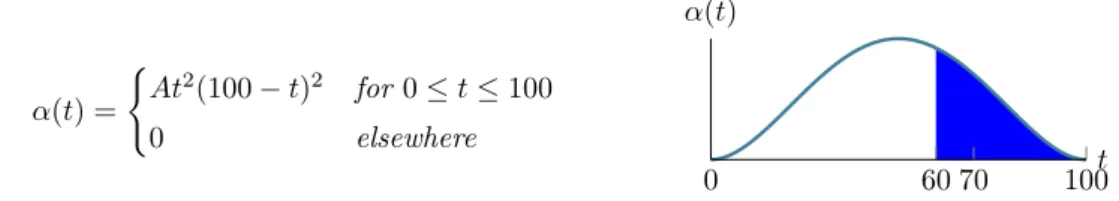
Let us suppose that we were able to build a "mortality" function of time α(t) from long records such as α(t) = ( At2_{(100 − t)}2 _{for 0 ≤ t ≤ 100} 0 elsewhere 0 60 70 100t α(t)

then the probability to die between two time intervals (t1, t2) is defined as (2.16).

Rephrasing the initial question in terms of conditional probability, it is the same as saying "what is the probability to die between 60 and 70 assuming to have lived to 60?". The formalization of such question is the following

P (60 ≤ t ≤ 70|t ≥ 60) = A Z 70 60 t2(100 − t)2dt A Z 100 60 t2(100 − t)2dt = 0.486

2.2.2 Total probability

We are now going to introduce the concept of Total Probability. Let us now assume we have

n mutually exclusive events {A1, A2, . . . , An} whose sum equals our universe. Let us have

another event B ⊂ S which intersects all (or a part of the) events Ai, i = 1, 2, . . . , n as in Fig. 2.3. B A1 A2 A3 A4 _A 5 · · · An−1 An

Figure 2.3: The event B intersects some of the events Ai which form the universe set.

From the set theory (see section2.1, properties of null and S) we know that B = BS, hence

B = B(A1+ A2+ · · · + An)

= BA1+ BA2+ · · · + BAn (2.19)

which probability, from the third corollary of the axioms of probability (since the events Ai are mutually exclusive) will result in

(25)

From (2.18) we can hence formalize the theorem of Total Probability:

P (B) = P (B|A1)P (A1) + P (B|A2)P (A2) + · · · + P (B|An)P (An) (2.21)

which is still true even if the sum of Ai is not S but is a superset of B. This is an important theorem since it provides the probability of a subset of mutually exclusive events just from the conditional probabilities P (B|Ai) and the probabilities of the single events P (Ai).

2.2.3 Bayes’ theorem

Now, from (2.18) we have that

P (AiB) = P (Ai|B)P (B) (2.22)

however, from the properties of the intersection between sets we have that P (AiB) = P (BAi), hence

P (AiB) = P (B|Ai)P (Ai) (2.23)

Putting (2.22) into (2.23) we obtain

P (Ai|B) = P (B|Ai)P (Ai)

P (B) (2.24)

and inserting (2.21) into the above we can formalize the Bayes’ theorem as follows

P (Ai|B) = P (B|Ai)P (Ai)

P (B|A1)P (A1) + P (B|A2)P (A2) + · · · + P (B|An)P (An)

(2.25)

Bayes’ Theorem - Discussion

Let us clarify this concept in comparison with the total probability: looking at Fig.2.3, let us suppose that every set Ai is a box containing both white and/or blue balls. The chance to pick a blue ball from a box Ai is described by the intersection between that box and the B set. Notice that not every box contains blue balls, and also there is a chance that some boxes do not contain white balls at all. Let us pick a random ball from any of the n boxes; suppose we know the number of balls available for each box and also we know the

rate between blue and white balls for each box, then the two theorems answer the

following questions:

• What is the chance that the extracted ball is blue? (Total Probability)

• Provided that we have extracted a blue ball, what is the chance that it comes from the

ithbox? (Bayes’ Theorem)

This last theorem also expresses the concept of an event’s a posteriori probability. This theorem is a keystone of filtering theory. It is indeed already possible to intuitively deline the bone structure of a filter by means of the Bayes’ theorem.

(26)

Let us suppose we want to know the real value of a certain process (e.g. position and velocity of a stone which leaves the hand of a thrower with a certain angle θ and a certain initial speed v) in real time through a series of measurements (e.g. camera images acquired during flight) which occur at a certain rate. Employing the Newton’s law to describe the trajectory of the stone, it would seem a simple deterministic problem, in which the state of the system can be described for each t by

             py(t) = kvk sin θ · t −1 2gt 2 px(t) = kvk cos θ · t vy(t) = kvk sin θ − gt vx(t) = kvk cos θ (2.26)

however, our model does not take into account a number of other factors that affect the actual state of our process, such as wind speed, air viscosity, stone shape, uncertainties on the initial (v, θ), etc. Hence, we can only guess that the position and velocity of the stone from t to t + 1 propagate as we would espect from (2.26). This guess can be translated into a cloud of possible positions more densely distributed near the center (our model guess) and more sparsely going outwards as in example 4, so that the probability of our estimation to be between certain boundaries is described by (2.16). The more accurate the model, the less sparse away from the center the cloud of points will be. This is called an a priori estimate of the system state.

After the state propagation, we take a measurement. Similarly to our model guess, the measurement is affected by uncertainties (e.g. circuit thermal noise). Finally, having our a

priori estimate of the state with a certain probability P (At+1) and a measurement event with a probability P (B), it is possible to fuse those two information in terms of a posteriori probability through the Bayes’ theorem. Just like in the example of the blue and white balls, we can intuitively rephrase our filtering problem as: "assuming we are given a measurement

of the state at time t+1, what is the probability that the true state comes from our a priori estimate At+1?". Hence our new state estimate will be another cloud of points distributed around our new guess with a probability P (At+1|B) described by (2.16), with an accuracy that in the following chapters (section3.2) will be proven higher than the one of the a priori estimate and the one of the measurement.

5 8 11.3 13 px

initial state

a priori

measurement

a posteriori

Figure 2.4: Focusing on a single state variable (e.g. px), we suppose our initial estimate of the state at time t is 5, with the uncertainty of this initial guess represented by the dashed bell curve. Then we propagate our initial guess through the model, getting our a priori estimate at t + 1. Notice that the uncertainty of the model negatively affects the initial guess. A at t + 1 we measure 13. The a posteriori estimate of the state is hence computed (red bell). Notice that this final result has its central value nearer the "most reliable" guess, which in this case is the measurement in comparison with the a priori estimate.

(27)

2.2.4 Independent events

Two events A, B ⊂ S are said independent if

P (AB) = P (A)P (B) (2.27) The independency of the two events implies the following statements:

• P (A|B) = P (A) • P (B|A) = P (B)

• P (A + B) = P (A) + P (B) − P (A)P (B)

Independency of n events and independency in pairs

If we have {A1, A2, . . . , An} independent events, then from (2.27) we can say

P (A1A2. . . An) = P (A1)P (A2) . . . P (An) (2.28)

However, if those events are independent in pairs

P (AiAj) = P (Ai)P (Aj) for every i 6= j (2.29) they are not automatically independent (see figure below).

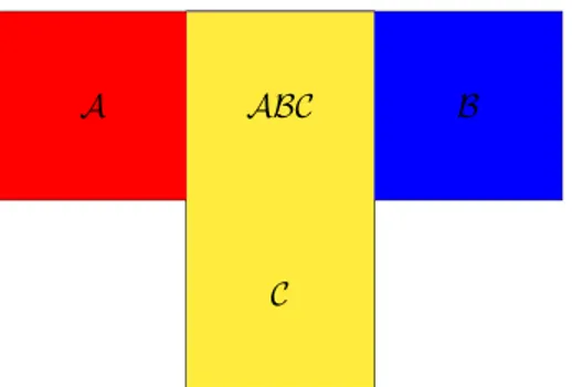
A B

C ABC

Figure 2.5: The events A,B and C are independent in pairs but not globally independent because AB = AC = BC = ABC, hence P (ABC) = P (AB) 6= P (A)P (B)P (C).

2.3 Random variables

Considering an experiment E : (S, F, P ) in which ξ ∈ S are outcomes and F is a field of subsets of S called events, we define a function x which domain is the universe set and the codomain is the real line R:

x(ξ) : S 7→ R (2.30)

(28)

2.3.1 The distribution function and the density function

Considering a number x ∈ R, the set {x ≤ x} represents another set of outcomes ξ such that

x(ξ) ≤ x (2.31)

which is the definition of an event (see section2.1.2).

Thus, we can define the probability of such event as a number which depends on x

Fx(x) = P {x ≤ x} (2.32)

defined for every x from −∞ to ∞. This is called the Distribution function of the random variable. For the sake of notation simplicity, the distribution functions of the r.v. x, y, z, . . . will be referred to F (x), F (y), F (z), . . . without fear of ambiguity.

The distribution function F (x) has the following properties (given without proof): • F (−∞) = 0, F (+∞) = 1

• F (x1) ≤ F (x2) for x1≤ x2 (nondecreasing for x)

• F (x+_{) = F (x) (continuous from the right)}

• P {x1< x ≤ x2} = F (x2) − F (x1) for x1< x2.

The derivative of the distribution function is the Density function

f (x) = dF (x)

dx (2.33)

However, the distribution function may not have a derivative ∀x, hence the following sections will shorly deal with continuous and discrete r.v.

Continuous type r.v.

Suppose F (x) to be a continuous function of x (and may have a countable number of corners). Then it follows from the second property of the distribution function that

f (x) ≥ 0 (2.34)

and from the first property Z ∞ −∞ f (x)dx = F (∞) − F (−∞) = 1 (2.35) F (x) = Z x −∞ f (ξ)dξ (2.36) Hence, F (x2) − F (x1) = Z x2 x1 f (x)dx (2.37)

(29)

which from the fourth property of the distribution function brings to

P {x1≤ x ≤ x2} =

Z x2

x1

f (x)dx (2.38)

Notice that we have finally estabilished a link between the random variables and the probability on the real line (cfr. 2.15and2.38), and that "integrable function of time α(t)" that we defined previously is nothing else than a density function.

Discrete type r.v.

Suppose now F (x) to be a discrete "staircase" type function with discontinuities at every countable xi. Each jump shall be defined by a probability

P {x = xi} = pi= F (xi) − F (x−_i ), i = 1, 2, . . . (2.39) and the distribution distribution function will be

F (x) =X

i

pi= F (∞) − F (−∞) = 1 (2.40)

Example 5. Let us consider a coin tossing experiment: S = {h, t} with the following

probabilities P {h} = p and P {t} = q. Let us suppose an unfair coin with q < p. Now let’s define the r.v. x by x(h) = 1, x(t) = 0 0 1 q 1 x F (x) 0 1 q p x f (x)

Since the experiment itself implies two possible outcomes, the distribution function is a staircase function. The density function is formed with the probabilities of each outcome as in (2.40).

2.3.2 Conditional distribution and density

It is now possible to extend the concept of conditional probability to the r.v.

Let us consider an event M ⊂ S, hence the conditional distribution of a r.v. x assuming M shall be

F (x|M) = P {x ≤ x|M} = P {x ≤ x, M}

P (M) (2.41)

where the set {x ≤ x, M} is the event of all the outcomes that satisfy both conditions

(30)

Furthermore, supposing x of continuous type we can define the conditional density function as

f (x|M) = dF (x|M)

dx (2.42)

2.3.3 Functions of one r.v.

When we talked about a r.v. x, we defined a function which domain is the universe set, and its range (codomain) is a set of real numbers Ix⊂ R. We now define another kind of function which takes a random variable as argument

y = g(x) (2.43)

by analogy with any other function which takes a real variable x as an argument, it is trivial to see that the domain of y is still S. Indeed, y is still a r.v.. Its distribution function is hence defined

F (y) = P {y ≤ y} = P {g(x) ≤ y} (2.44)

and its density function

f (y) = dF (y)

dy (2.45)

Similarly to x, the range of y so that {g(x) ≤ y} is Iy. Hence we can state that

g(x) ≤ y ⇐⇒ x ∈ Iy (2.46) so that

F (y) = P {y ≤ y} = P {x ∈ Iy} (2.47)

The following example is useful to fix this concept and also to better appreciate the implications of the definition of a function of one r.v..

Example 6. Let us consider the experiment of the fair six-faced die as in example2. Hence

for S = {1, 2, . . . , 6} = {f1, f2, . . . , f6} we have that

P {fi} =1_/₆ _for _{i = 1, 2, . . . , 6}

Now let us select our r.v. so that x(fi) = i − 3, we hence have

−2 −1 0 1 2 3 0 1 x F (x) −2 −1 0 1 2 3 1_/₆ x f (x)

(31)

If we choose y = x2_{, the r.v. will take those values {0, 1, 4, 9}} 0 1 4 9 1_/₆ 3_/₆ 5_/1₆ x F (x) 0 1 4 9 1_/₆ 2_/₆ x f (x)

Notice how, out of the same experiment, the choice of the random variable affects the distribution and density functions of the outcomes.

Unlike the example above, the determination of a function of one r.v. density is not always so trivial. This is expecially true when dealing with r.v. of continuous type. Hence, the following theorem will deal with the determination of f (y). This fundamental theorem can be applied to any function of one r.v..

Theorem 1. Let us consider a function of one r.v. as y = g[x]

in order to find f (y) it is necessary to solve

y = g(x)

for each root of x in terms of y, consdering that x1, x2, . . . , xn, . . . are all the its real roots

y = g(x1) = g(x2) = · · · = g(xn) = . . . Then, f (y) = f (x) |g0 (x1)| + · · · + f (x) |g0 (xn)| + . . . (2.48) with g0(x) =dg(x) dx

Also, its conditional density f (y|M) is a simple extension of (2.48) prior the knowledge of f (x|M) as follows f (y|M) = f (x|M) |g0 (x1)| + · · · +f (x|M) |g0 (xn)| + . . . (2.49) Proof:

(32)

g(x)

f (x)

y y + dy

x1 x2 x3 x

Suppose that y = g(x) has three roots x1, x2, x3. For a dy sufficiently small we have

P {y < y < y + dy} = P {y < g(x) < y + dy} = f (y)dy

which is true for (see figure above, blue filled areas in f (x))

x1< x < x1+ dx1, x2− dx2< x < x2, x3< x < x3+ dx3

so that

P {y < y < y + dy} = P {x1< x < x1+ dx1}

+ P {x2− dx2< x < x2}

+ P {x3< x < x3+ dx3}

Also, for dxi sufficiently small

P {x1< x < x1+ dx1} = f (x1)|dx1|

P {x2− dx2< x < x2} = f (x2)|dx2|

P {x3< x < x3+ dx3} = f (x3)|dx3|

Considering that we defined g0(x) =dg(x)_/_dx₌ dy_/_dx _{we obtain}

f (y)dy = f (x1) |g0 (x1)| dy + f (x2) |g0 (x2)| dy + f (x3) |g0 (x3)| dy

2.3.4 Expectation, variance and moments of a r.v.

In this section we introduce the most important parameter in terms of application of probability theory and r.v.: the Expectation. This single paramter will be extensively used in most of the following chapters, and its properties and geometrical interpretations are fundamental to the filtering theory in order to define robust mathematical instruments such as optimal state observers.

(33)

The Expectation or expected value of a r.v. x is written in the following form E [x] or ηx or η

and it is defined in its continuous form as E [x] =Z

∞

−∞

xf (x)dx (2.50)

and in its discrete form as

E [x] =X n xnP {x = xn} = X n xnpn (2.51)

Example 7. Let us consider once more the six-faced die experiment. The universe set and

the probabilities associated to each outcome have been defined in example6. However, this time we define for simplicity the r.v. x(fi) = fi. If we apply the discrete form of the expected value (2.51) to our experiment we obtain

E [x] =X n

xnpn = 1

6(1 + 2 + 3 + 4 + 5 + 6) = 3.5

which should make more clear why the expectation is also called "mean". More generally, for experiment with a non-infinite number of trials n, we can define

E [x] ' x1(ξ) + · · · + xn(ξ)

n (2.52)

which is the frequency interpretation of the expectation.

In the figure below we reported the example above performed with 1000 die throws. For each kth _{throw the average value of the 1, ..., k − 1, k results is computed. Notice that, for an}

increasing number of throws, the average value tends to the expectation, thus confirming the frequency interpretation. Eventually, the computed average will be equal to the expectation for n → ∞. It comes along that for evenly distributed density functions the expectation, the median and the most likely outcome are equal to each other.

0 500 1,000 3.5 7 throws av er ag e

To emphasize the point above, consider the right-skewed distribution f (x) = |x|e−x in the next figure. Notice how the most likely value, the median and the expectation occupy different places in the distribution.

(34)

Median

E [x]

Most likely (Mode)

0 xl xm xη

x f (x)

with the mode defined as the the xl where f (x) is maximum and the median defined as

P {x ≤ xm} = F (xm) =1_/₂_{or, more explicitly, as the value x}_m _{so that}

Z xm 0 |x|e−xdx = 1 2 assuming 0 ≤ x < ∞. Conditional Expectation

The conditional expected value of a r.v. assuming an event M ⊂ S is simply given by E [x|M] =Z ∞

−∞

xf (x|M)dx (2.53)

with its discrete form

E [x|M] =X k

xkP {x = xk|M} (2.54)

Expectation of g(x)

Let us consider a function of one r.v. as introduced in section2.3.3, such as y = g(x). From the definition of expectation

E [y] =Z

∞

−∞

yf (y)dy (2.55)

The following theorem will allow the definition of such expectation in terms of f (x).

Theorem 2. The expecation of g(x) in terms of f (x) is expressed as follows

E [g(x)] =Z ∞

−∞

g(x)f (x)dx (2.56)

and its discrete form is

E [g(x)] =X k

g(xk)P {x = xk} (2.57)

Proof: From the proof of Theorem 1we have

(35)

If we multiply on both sides for y we obtain

yf (y)dy = g(x1)f (x1)dx1+ g(x2)f (x2)dx2+ g(x3)f (x3)dx3

for each element yf (y)dy there is a number of differential elements in g(x)f (x)dx. Since the two differential dx and dy occupy two orthogonal spaces (see figure in proof of Theorem1), they do not overlap. Hence (2.55) and (2.56) are equal.

The above theorem allows to define an important property of the expectation operator.

Additivity

From Theorem 2we can conclude that for

g(x) = g(x1) + · · · + g(xn) (2.58) then E [g(x1) + · · · + g(xn)] =E [g(x1)] + · · · +E [g(xn)] (2.59) Most importantly E [ax + b] = aE [x] + b, with a, b ∈ R (2.60) Variance

The concept of variance gives a notion of how much the possible outcomes x(ξi) are dispersed around the mean valueE [x]. Such quantity is expressed as

σ2=E [(x − E [x])2] = Z ∞

−∞

(x −E [x])2f (x)dx (2.61) and in its discrete form

σ2=X n

(xn−E [x])2· P {x = xn} (2.62)

To clarify this concept, imagine that the function f (x) is a certain non-uniform mass (such as an oddly shaped stone). Every dx of such mass is a small-at-will portion of it. In this case, if the expectation value E [x] matches the center of gravity of such object, its variance equals the moment of intertia of those dx masses, thus defining how those portions are distributed around the center of gravity.

Thanks to (2.60), we can obtain the following important relationship

σ2=E [(x − E [x])2]

=E [x2− 2xE [x] + E2_[x]]

=E [x2] − 2E [x]E [x] + E2[x]

=E [x2] −E2[x] (2.63)

(36)

Moments of order k and central moments

Similarly to the definition of variance, we can raise the exponential inside (2.61) to obtain moments of higher order.

E [(x − E [x])k ] =

Z ∞

−∞

(x −E [x])kf (x)dx (2.64) where the presence of the mean value on the left side of the equation makes them central

moments.

More generally, we can define the moments and absolute moments respectively as

E [xk ] = Z ∞ −∞ xkf (x)dx (2.65) E [|x|k ] = Z ∞ −∞ |x|kf (x)dx (2.66)

In particular, it is worth mentioning that the 3rd _{and 4}th _{central moments are called}

skewness and kurtosis respectively. Their properties are extensively used in statistics, but

are not covered in this dissertation.

2.3.5 Characteristic function

The characteristic function of a r.v. x can be expressed as the Fourier transform of its density function f (x) (with a minus sign). This mathematical tool is fundamental to simplify certain operations that can be done with r.v. and, in the next chapters, with stochastic processes. This brief section contains a set of definitions and properties of such this particular mathematical tool.

Definition 3 (Characteristic function). The characteristic function of a r.v. x is

φ(ω) =E [ejωx] (2.67)

where,

ejωx= cos(ωx) + j sin(ωx) (2.68)

and from the definition of expectation,

φ(ω) = Z ∞

−∞

ejωxf (x)dx (2.69)

Starting from (2.69), it is possible to obtain the inversion formula that allows to find the probability density function known the characteristic function of the related r.v.

Definition 4 (Inversion formula).

f (x) = 1

2π Z ∞

−∞

(37)

Proof: Starting from the definition of a delta function as 1 2π Z ∞ −∞ e−jωxdω = δ(ω) (2.71)

we can say that

1 2π Z ∞ −∞ φ(ω)e−jωxdω = 1 2π Z ∞ −∞ e−jωx Z ∞ −∞ ejωyf (y)dydω = 1 2π Z ∞ −∞ f (y) Z ∞ −∞ ejω(y−x)dωdy = Z ∞ −∞ f (y)δ(x − y)dy = f (x)

Let us now introduce the convolution operator: given to functions f1(x) and f2(x), the

convolution of those two functions is the new function f (x):

f (x) = Z ∞ −∞ f1(ξ)f2(x − ξ)dξ = Z ∞ −∞ f1(x − ξ)f2(ξ)dξ = f1(x) ∗ f2(x) (2.72)

This concept will be discussed more thoroughly in the following section (Theorem 4), for now we just formally define it to give the following theorem

Theorem 3 (Convolution theorem for characteristic functions). If φ1(ω) and φ2(ω)

are respectively the characteristic functions of f1(x) and f2(x) then the characteristic function

of their convolution f (x) = f1(x) ∗ f2(x) is φ(ω) = φ1(ω)φ2(ω) (2.73) Proof: Z ∞ −∞ ejωxf (x)dx = Z ∞ −∞ ejωx Z ∞ −∞ f1(y)f2(x − y)dydx = Z ∞ −∞ f1(y) Z ∞ −∞ ejωxf2(x − y)dxdy for x − y = τ Z ∞ −∞ f1(y)ejωy Z ∞ −∞ ejωτf2(τ )dτ dy = φ1(ω)φ2(ω)

2.3.6 Two r.v. and functions of two r.v.

This section contains important notions that will be useful to build the concept of optimal

(mean-square) estimators. However, many of the properties of two r.v. and functions of two

r.v. are beyond the aim of this dissertation, hence many concepts are given "as is" and this section may very well seem dry. For more in-depth analysis please refer to [1] (Chapters 6 and 7).

(38)

Joint distribution and density functions

Let us consider two r.v. x and y. Due to (2.32), each one of these has its own distribution function F (x) and F (y). Now, let us consider the following set

{x ≤ x}{y ≤ y} = {x ≤ x, y ≤ y} (2.74)

which represents the set of all ξ such that x(ξ) ≤ x and y(ξ) ≤ y are both verified. Hence, we can define a probability of this event as the joint distribution function

F (x, y) = P {x ≤ x, y ≤ y} (2.75)

As the reader may already expect, since the joint distribution function depends on two r.v., the joint density function will consist in partial derivatives as follows

f (x, y) = ∂

2_{F (x, y)}

∂x∂y (2.76)

Generally speaking, it is possible to deline the joint statistics of two r.v. rewriting (2.75) as the set of all outcomes ξ that belong to a region D of the xy plane, such that

F (x, y) = P {(x, y) ∈ D} =

Z Z

D

f (x, y)dxdy (2.77)

which, extended to the whole plane becomes

F (x, y) = Z x −∞ Z y −∞ f (ξ, ρ)dξdρ (2.78)

for ξ ≤ x and ρ ≤ y, and

Z ∞

−∞

Z ∞

−∞

f (x, y)dxdy = 1 (2.79)

It comes along that the definition of a distribution function of a single r.v. can be expressed in terms of two r.v. as a marginal distribution

F (x) = F (x, ∞) = Z ∞ −∞ Z x −∞ f (ξ, y)dξdy (2.80)

Differentiating the above with respect to x it is possible to obtain the marginal density

f (x) =

Z ∞

−∞

f (x, y)dy (2.81)

Joint conditional distribution, density, total probability and Bayes’ theorem

From equation (2.41) we can define the conditional distribution of a r.v. y assuming an event M.

F (y|M) = P {y ≤ y, M}

(39)

Now, let us see the event M in terms of a r.v. x

F (y|x ≤ x) = P {y ≤ y, x ≤ x}

P {x ≤ x} (2.83)

placing (2.75) into the above we obtain

F (y|x ≤ x) =F (x, y)

F (x) (2.84)

Differentiating the equation above with respect to y and considering (2.78) and (2.80), we obtain the conditional density function as follows

f (y|x ≤ x) = ∂F (x, y)/∂y F (x) = Rx −∞f (ξ, y)dξ R∞ −∞ Rx −∞f (ξ, y)dξdy (2.85)

Considering an event localized on a single outcome such as M = P {x = x}, the equation above, thanks to (2.81), becomes

f (y|x = x) = _R∞f (x, y) −∞f (x, y)dy

= f (x, y)

f (x) (2.86)

From (2.81) and (2.86) we can once more find the total probability

f (y) =

Z ∞

−∞

f (y|x = x)f (x)dx (2.87)

and the Bayes’ theorem

f (y|x = x) = f (x|y = y)f (y)

f (x) (2.88)

Joint conditional expectation

Let us now define the concept of joint conditional expectation, which is referred to as

E [y|x] = E [y|x = x(ξ)] (2.89)

Considering that the conditional expectation of a r.v. y assuming an event M can be stated as

E [y|M] =Z ∞

−∞

(40)

the joint conditional expectation shall be

E [y|x = x] =Z ∞

−∞

yf (y|x)dy (2.91)

which can be intended as the center of gravity of the vertical strips (x, x + dx) of a function

g(x).

Remark 1. The expectation of E [y|x] satisfies the following equation

E [E [y|x]] = E [y] (2.92) Proof: E [E [y|x]] =Z ∞ −∞ E [y|x = x]f(x)dx = Z ∞ −∞ Z ∞ −∞

yf (y|x = x)f (x)dxdy from (2.91)

= Z ∞ −∞ Z ∞ −∞ yf (x, y)dxdy from (2.86) = Z ∞ −∞ yf (y)dy from (2.81)

This fundamental remark implicitly delines the concept of estimator. Let us intuitively deline this concept: if we consider our system state as the r.v. y and some measurements relative to that process as another r.v. x, we can see that the expecation of such r.v. is equal to the expectation of the center of gravity of the vertical strips of a g(x) function which can be chosen as a particular transformation from the measurement space to the system state space. In short, the expectation of the center of gravity of the system states yk assuming

the measurements xk is equal to the expectation of the system’s state for each kthtime step.

Thus, given a set of measruement related to the system state through g(x), it is possible to obtain an estimate of the system’s state.

Independent r.v.

Starting from the concept of events independency expressed in (2.27), and also from (2.74) and (2.75) we obtain the following relationships

P {x ≤ x}{y ≤ y} = P {x ≤ x, y ≤ y} (2.93)

F (x, y) = F (x)F (y) (2.94)

f (x, y) = f (x)f (y) (2.95)

Hence, if x and y are independent, their joint conditional densities will be

f (y|x) = f (y), f (x|y) = f (x) (2.96)

Functions of two r.v.

In this section the concept of function of one r.v. (see section2.3.3) is extended to two r.v. Let us define a r.v. z so that

(41)

z = g(x, y) (2.97) with its distribution function

F (z) = P {z ≤ z} (2.98)

The region of the plane xy in which (2.98) is satisfied is denoted as Dz. Hence the following

F (z) = P {z ≤ z} = P {(x, y) ∈ Dz} = Z Z

Dz

f (x, y)dxdy (2.99)

defines the relationship between the distribution and density functions of z.

Now, let us define a typical example of function of two r.v.: z = x + y. On the plane xy we define a region Dz such that

x + y ≤ z

x + y = z

Dz

x y

To find F (z) we have to integrate using suitable strips until we meet the line x + y = z on the xy plane (or x = z − y), so that

F (z) = Z ∞ −∞ Z z−y −∞ f (x, y)dxdy (2.100)

which becomes, if we differentiate with respect to z (from the fundamental theorem of calculus)

f (z) =

Z ∞

−∞

f (z − y, y)dy (2.101)

Let us now assume that x and y are independent, hence from (2.95) we have

f (z) = Z ∞ −∞ f (z − y, y)dy = Z ∞ −∞ f (z − y)f (y)dy (2.102)

This last equation provides a fundamental theorem that will be enunciated here

(42)

their sum z = x + y equals the convolution of their densities fz(z) = Z ∞ −∞ fx(x)fy(z − x)dx = Z ∞ −∞ fx(z − y)fy(y)dy (2.103)

Proof: The last term of this equation has been proven through (2.100)-(2.102). The second term can be proven analogously considering y = z − x instead of x = z − y in (2.100).

The concept of convolution may appear rather obscure from (2.103). The subscripts x, y and z under each density function have been added to facilitate its comprehension. In its general form, the convolution is defined as follows

(f ∗ g)(t) = Z ∞

−∞

f (τ )g(t − τ )dτ (2.104)

Hence, considering a fixed t, the result is the area underlying the function f (∗)g(∗), where

g(∗) is reversed and shifted by an amount t along the integration axis. By varying t from

−∞ to ∞, g(∗) is translated from left to right, and the integral function is computed for each

t. It becomes clear now that, while shifting g(∗), anywhere the domains of the two functions

are not overlapping, the value of the integral will be zero. Otherwise it will be equal to the area underlying f (τ )g(t − τ ). It should also be clear now why the result does not depend on which function is held fixed and which one is shifted along the integration axis, so that

(f ∗ g)(t) = Z ∞ −∞ f (τ )g(t − τ )dτ = Z ∞ −∞ f (t − τ )g(τ )dτ (2.105)

Example 8. In a dice-based game, a player is asked to choose to throw either one

twelve-sided die (1d12) or the sum of two six-faced dice (2d6). Suppose the aim of the game is to obtain the most consistent results over a large number of throws, what is the best choice? (e.g. in a combat-based tabletop game, if the two dice choices represent the potential damage of two different weapons, the player may want to choose the strongest one). At first sight one might say that the best choice is 2d6 since the minimum obtainable result is 2 against 1 of the

1d12 die. This is a good point, and in the end it would lead to the best choice, nonetheless let

us examine it in terms of r.v. to find out if this is really the main advantage of 2d6 over the

1d12. Let us define the probability profiles of the two dice:

1d12 = {1, 2, . . . , 12}, P {ξi} = {1/12} for i = 1, 2, . . . , 12 (2.106) 1 2 3 4 5 6 7 8 9 10 11 12 0 1 x F (x) 1 2 3 4 5 6 7 8 9 10 11 12 1_/₁₂ x f (x) 1d6 = {1, 2, . . . , 6}, P {ρi} = {1_/₆_} _for _{i = 1, 2, . . . , 6}