38100 Povo — Trento (Italy), Via Sommarive 14 http://dit.unitn.it/
R-EVO
A REACTIVE EVOLUTIONARY ALGORITHM
FOR THE MAXIMUM CLIQUE PROBLEM
Roberto Battiti, Mauro Brunato
May 31, 2007
R-
EVO
: a Reactive Evolutionary Algorithm for the
Maximum Clique Problem
Roberto Battiti and Mauro Brunato
Abstract—An evolutionary algorithm with guided mutation (EA/G) has been proposed recently for solving the maximum clique problem. In the framework of estimation-of-distribution algorithms (EDA), guided mutation uses a model distribution to generate the offspring by combining the local information of solutions found so far with global statistical information. Each individual is then subjected to a Marchiori’s repair heuristic, based on randomized extraction and greedy expansion, to ensure that it represents a legal clique.
The novel reactive and evolutionary algorithm (R-EVO) pro-posed in this paper starts from the same evolutionary framework but considers more complex individuals, which modify tentative solutions by local search with memory, in the reactive search framework. In particular, the estimated distribution is used to periodically initialize the state of each individual based on the previous statistical knowledge extracted from the population. We demonstrate that the combination of the estimation-of-distribution concept with reactive search produces significantly better results than EA/G and is remarkably robust w.r.t. the setting of the algorithm parameters.
R-EVO adopts a drastically simplified low-knowledge version of reactive local search (RLS), with a simple internal diversi-fication mechanism based on tabu-search, with a prohibition parameter proportional to the estimated best clique size.
R-EVOis competitive with the more complex full-knowledge
RLS-EVO which adopts the original RLS algorithm. For most of the benchmark instances, the hybrid scheme version produces significantly better results than EA/G for comparable or smaller CPU times.
Index Terms—Maximum Clique, Reactive Search, Estimation of Distribution, guided mutation
I. INTRODUCTION
P
ROBLEM-solving systems, both natural and artificial,can be made more efficient by working along different directions. One direction measures the complexity of a single problem-solving entity (an individual in the population in GA terms), another one is the number of individuals and the amount of their mutual interaction. For example, an individual may be very simple, leaving to mutation, cross-over and selec-tion the work of exploring and exploiting the fitness surface, or it may become more complex, embodying for example repair procedures [1], or elements of local search, as in memetic algorithms [2], [3]. The interaction in the population can be indirect, based on the current fitness of the individuals which influences the reproduction, or more direct and based on both global and local information, see for example the “particle swarm” technique where each member of the swarm is updated based on the global best position and the individual best [4]. Interaction through explicit statistical models of
Work supported by the project Bionets (IST-027748) funded by the FET Program of the European Commission.
the promising solutions is advocated in the “estimation of distribution algorithms” (EDA), see for example [5]–[9]. In a different community, methods to combine solutions have been designed with the term “scatter search” [10], [11], showing the advantages provided by intensification and diversification mechanisms that exploit adaptive memory, drawing on foun-dations that link scatter search to tabu search [12].
While a complete coverage of the tradeoffs between com-plexity of the individual population members and comcom-plexity of their interaction is beyond the scope of this paper (some useful historical references can be found in the cited papers), this work is motivated by a recent evolutionary algorithm with guided mutation for the maximum clique proposed in [13], where the authors obtain state-of-the-art results in the area of evolutionary algorithms for the problem, by improving upon Marchiori’s results [1], [14] and upon an advanced EDA algorithm like MIMIC [15].
The Maximum Clique problem in graphs (MC for short) is a paradigmatic combinatorial optimization problem with relevant applications [16], including information retrieval, computer vision, and social network analysis. Recent inter-est includes computational biochemistry, bio-informatics and genomics, see for example [17], [18]. The problem is NP-hard and strong negative results have been shown about its approximability [19], making it an ideal test-bed for search heuristics.
LetG = (V, E) be an undirected graph, V = {1, 2, . . . , n}
its vertex set, E ⊆ V × V its edge set, and G(S) = (S, E ∩
S × S) the subgraph induced by S, where S is a subset of V . A graph G = (V, E) is complete if all its vertices are
pairwise adjacent, i.e., ∀i, j ∈ V, (i, j) ∈ E. A clique K
is a subset of V such that G(K) is complete. The Maximum
Clique problem asks for a clique of maximum cardinality. The initial motivation of this work was to assess whether the incorporation of Reactive Search ideas developed in [20], [21] into an evolutionary approach could lead to a competitive technique. Furthermore, we wanted to confirm whether the advantage of the technique persisted after radical simplifi-cations of the Reactive Search algorithm. The simplification has been motivated by a note in the cited paper [13], stating that, while more effective, “reactive local search is much more complicated and sophisticated than EA/G”. We propose here a radically simplified reactive scheme, hybridized with an EDA approach, which maintains a significant advantage over EA/G, when both clique sizes and CPU times are considered.
Reactive Search, see [22], [23] for seminal papers, advocates the use of machine learning to automate the parameter tuning process and make it an integral and fully documented part of the algorithm. Learning is performed on-line, and therefore
task-dependent and local properties of the configuration space
can be used. In this way a single algorithmic framework maintains the flexibility to deal with related problems through an internal feedback loop that considers the previous history of the search.
The main novelties introduced by the R-EVOalgorithm are:
• While guided mutation is used to generate new
individ-uals in EA/G, individindivid-uals which are then subjected to a repair heuristics to create a legal clique, the model obtained by estimation of distribution is used to create
new individuals in R-EVO
• Memetic evolution: each individual is subjected to a short
run of intelligent local search (prohibition-based reactive search) which considers the given individual as a starting point.
• Extreme simplification through the design of a
low-knowledge version of the reactive local search algorithm: instead of the complete memorization of previous so-lutions, only the best cliques (up to a given tolerance
parameter ∆) are used to derive a probabilistic model
of the fittest individuals and to self-tune the prohibition period on a specific instance.
• Simplification of the model derivation. The model is
not obtained through an exponentially weighted moving average but in a parameter-less manner from the best
previous solutions (within tolerance parameter∆).
• Proposal of number of iterations and prohibition period
scaled according to the best clique-size estimated at run-time on a specific instance.
II. EVOLUTION WITHGUIDEDMUTATION
Estimation of Distributions (EDA) algorithms [5]–[9], [24] have been proposed in the framework of evolutionary com-putation for modeling promising solutions in a probabilistic manner, and for using such models to produce the next genera-tion. A survey in [25] considers population-based probabilistic search algorithms based on “modeling promising solutions by estimating their probability distribution and using the model to guide the exploration of the search space.” The main idea of model-based optimization is to create and maintain a model of the problem, whose aim is to provide some clues about the problem’s solutions. If the problem is a function to be minimized, for instance, it is helpful to think of such model as a simplified version of the function itself; in more general settings, the model can be a probability distribution defining the estimated likelihood of finding a good quality solution at a certain point.
To solve a problem, we resort to the model in order to generate a candidate solution, then check it. The result of the check shall be used to refine the model, so that the future generation is biased towards better and better candidate solutions. Clearly, for a model to be useful it must provide as much information about the problem as possible, while being somehow “more tractable” (in a computational or analytical sense) than the problem itself.
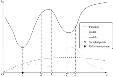
Although model-based techniques can be used in both discrete and continuous domains, the latter case better supports our intuition. In Fig. 1 a function (continuous line) must
Unknown optimum O Function 1 2 model model Sampled points x f(x) e a b c d
Fig. 1. Model-based search: one generates sample points from model1 and
updates the generative model to increase the probability for point with low cost values (see model2). In pathological cases, optimal pointe runs the risk
of becoming more and more difficult to generate (figure from [21]).
(learning) Generation Long−term memory Feedback Memory Sample Model
Fig. 2. Model-based architecture: a generative model is updated after learning from the last generated samples and the previous long-term memory (figure from [21]).
be minimized. An initial model (the dashed line) provides a prior probability distribution for the minimum (in case of no prior knowledge, a uniform distribution can be assumed). Based on this estimate, some candidate minima are generated
(points a through d), and the corresponding function values
are computed. The model is updated (dotted line) to take into account the latest findings: the global minimum is more likely
to occur around c and d, rather than a and b. Further
model-guided generations and tests shall improve the distribution:
eventually the region around the global minimum e shall be
discovered and a high probability density shall be assigned to its surroundings. The same example also highlights a possible drawback of na¨ıf applications of the technique: assigning a
high probability to the neighborhood of c and d could lead
to a negligible probability of selecting a point near e, so the
global minimum would never be discovered. The emphasis is on intensification (or exploitation) of the search. This is why, in practice, the models are corrected to ensure a significant probability of generating points also in unexplored regions.
The scheme of a model-based search approach, see also [26], is presented in Fig. 2. Represented entities are:
• a model used to generate sample solutions,
• a memory containing previously accumulated knowledge about the problem (previous solutions and evaluations). The process develops in an iterative way through a feedback loop were new candidates are generated by the model, and their evaluation —together with memory about past states— is used to improve the model itself in view of a new generation. The design choices consist of defining a suitable generative model, and an appropriate learning rule to favor generation of superior models in the future steps. The simple model considered in this paper is as follows. The search space
X = {0, 1}n is the set of all binary strings of length n, the
generation model is defined by ann-tuple of parameters
p= (p1, . . . , pn) ∈ [0, 1]n,
wherepiis the probability of producing1 as the i-th bit of the
string and every bit is independently generated. One way to look at the model is to “remove genetics from the standard genetic algorithm” [6]: instead of maintaining implicitly a statistic in a GA population, statistics are maintained explicitly
in the vector(pi).
The initial state of the model corresponds to indifference
with respect to the bit values:pi= 0.5, i = 1, . . . , n. In the
Population-Based Incremental Learning (PBIL) algorithm [6] the following steps are iterated:
1. Initialize p; 2. repeat:
3. Generate a sample set S using the vector p;
4. Extract a fixed number ¯S of the best solutions from S; 5. for each sample s= (s1, . . . , sn) ∈ ¯S:
6. p ←(1 − λ)p + λs,
where λ is a learning rate parameter (regulating exploration
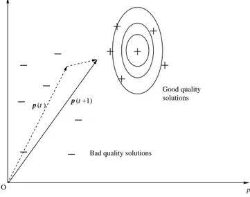
versus exploitation). The moving vector p can be seen as representing an exponentially weighted moving average of the best samples, a prototype vector placed in the middle of the cluster providing the recently-found best quality solutions. As a parallel with machine learning literature, the update rule is similar to that used in Learning Vector Quantization, see [27]. Variations include moving away from bad samples in addition to moving towards good ones. A schematic representation is shown in Fig. 3.
Estimates of probability densities for optimization consider-ing possible dependencies in the form of pairwise conditional probabilities are studied in [15]. Their MIMIC technique (Mutual-Information-Maximizing Input Clustering) aims at estimating a probability density for points with value below a given threshold (remember that the function is to be
min-imized). These more complex models have been considered
for the maximum clique problem in [13], which demonstrates inferior performance with respect to the simpler PBIL, in spite of added computational overhead.
The EA/G algorithm proposed in [13] for the maximum clique problem is based on the following principles:
• Use of the PBIL algorithm [5] to create a model of the
fittest individuals created in the population.
• Use of a guided mutation operator to produce the
off-spring. This is motivated by the “proximate optimality principle” [28] which assumes that good solutions tend to have similar structures. Global statistical information
t ( )t
−
O−
−
−
−
−
−
+
+
+
+
+
+
Good quality solutionsBad quality solutions
p p 2 1 p ( +1) p
Fig. 3. PBIL: the “prototype” vector p gradually shifts towards good quality solutions (qualitative example in two dimensions).
is extracted through EDA from the previous search and
represented as a probability model (a vectorp)
character-izing the distribution of promising solutions in the search space. A new individual is moved in a stochastic manner towards the center of the model. In detail, for each bit of the binary string describing the individual, one flips a coin
with head probabilityβ. If head turns up, the specific bit
is set to 1 with probabilitypi, to 0 otherwise. Ifβ = 1,
the string is sampled from the probability model p.
• Use of a lower bound on the maximum clique (size of
best clique found so far) to search for progressively larger cliques.
• Use of Marchiori’s repair heuristic [1] to create a legal
clique (some of the internal connections can be missing in the individual created with guided mutation) and to extend it in a greedy manner until a maximal clique is reached.
Fig. 4 outlines the EA/G code. The algorithm accepts as
input the population size N and some parameters described
below. The guided mutation operator described above is
im-plemented in function Mutation, while Marchiori’s repair
heuristic is performed by function Repair. The algorithm
works by maintaining a population of size N . At each step,
theM (equal to N/2 in the cited paper) fittest individuals are
kept, while the others are replaced by repaired mutations of the fittest individual. This is achieved in the pseudo-code by sorting individuals according to their fitness (line 15) and by
using the first one, x1, for generation of others (lines 18–20).
Elementsx2, . . . , xM do not generate offspring, but participate
to the PBIL model update (line 17). If a new population is to be generated (for instance, when a larger clique is found, or population converges to a single individual), new individuals
are selected among strings of length Sbest + 1 . . . Sbest+ ∆
(whereSbest is the lower bound on the maximum clique size,
i.e., the size of the best clique found so far) and the pi
distribution is reset (lines 9–13). The PBIL model is initialized at line 13 and updated by a moving average at line 17.
1. function EA/G(N , M , ∆, λ, β, α) 2. t ← 0; 3. pickx ∈ Ω; 4. Qbest ←Repair(x, α); 5. Sbest← |U |; 6. restart← true; 7. repeat
8. ifrestartor all xi’s are equal 9. fori ← 1, . . . , N 10. pickx ∈S Sbest+∆ j=Sbest+1Ωj; 11. xi ←Repair(x, α); 12. fori ← 1, . . . , n 13. pi ←P N j=1x j i/N ; 14. restart← false 15. SortBySize (xi,i = 1, . . . , N ); 16. fori ← 1, . . . , n 17. pi ← (1 − λ)pi+ λP M j=1x j i/M ; 18. fori ← M + 1, . . . , N 19. x ←Mutate(x1, (pi),β); 20. xi ←Repair(x, α);
21. if (size of fittest individual) > Sbest 22. Qbest ← new maximum clique; 23. Sbest ← |Qbest|;
24. restart← true;
25. t ← t + 1
26. until stopping condition
Fig. 4. The EA/G algorithm for the Maximum Clique problem.
III. ALOW-KNOWLEDGE REACTIVE LOCAL SEARCH
ALGORITHM
A Reactive Local Search (RLS) algorithm for the solution of the Maximum-Clique problem is proposed in [20], [29] and obtains state-of-the-art results in computational tests on the
second DIMACS implementation challenge1.
RLS is based on local search complemented by a feed-back (history-sensitive) scheme to determine the amount of diversification. The reaction acts on the single parameter that decides the temporary prohibition of selected moves in the
neighborhood. In detail, given the prohibition parameter T ,
after being moved (added to the clique or dropped from it)
a node remains prohibited for the nextT iterations. We shall
refer to non-prohibited nodes as allowed nodes.
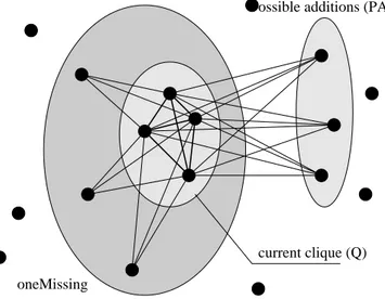
In local search algorithms for MC, the basic moves consist of the addition to or removal of single nodes from the current clique. A swap of nodes can be trivially decomposed into two separate moves. The local changes generate a search trajectory
X{t}, the current clique at different iterations t. Two sets
are involved in the execution of basic moves: the set of the
possible additions (PA) which contains nodes connected to all the elements of the clique, and the set of the level neighbors
oneMissingcontaining the nodes connected to all but one element of the clique, see Fig. 5.
The RLS algorithm [20] is presented in Fig. 6. It consists of a local search loop; every iteration basically
1http://dimacs.rutgers.edu/Challenges/
current clique (Q) oneMissing
Possible additions (PA)
Fig. 5. Neighborhood of current clique.
1. functionRLS 2. t ← 0; T ← 1; tR ← 0; Initialization 3. Q ← ∅; Qbest ← ∅; Sbest ← 0; tb ← 0; 4. repeat 5. T ←MemoryReaction(Q, T ); 6. Q ←BestNeighbor(Q); 7. t ← t + 1; 8. if f (Q) > Sbest 9. Qbest ← Q; 10. Sbest← |Q|; 11. tb ← t; 12. if t − max{tb, tR} > A 13. tR ← t; 14. Restart();
15. untilSbest is acceptable
16. or maximum iterations reached;
Fig. 6. The RLS algorithm for the Maximum Clique problem.
calls the BestNeighbor function that provides the fittest
neighboring configuration, given the current one. Function
BestNeighbor, outlined in Fig. 7, alternates between ex-pansion and plateau phases, and it selects the nodes among
the allowed ones which have the highest degree in PA. In
particular, the function searches for an allowed node within
PAwith the highest degree within PAitself (lines 4–6). If no
such node is available, then it tries to remove an allowed node
from the clique which would maximally increasePA(lines 10–
11). If all such nodes are prohibited, then it proceeds removing a random node from the clique (line 13).
The part that differentiates RLS from other local search
mechanisms is functionMemoryReaction, which maintains
the history of the search by storing each visited cliqueQ (or
a suitable fingerprint) into a dictionary structure, e.g., a hash table, together with some details, such as the number of times a given clique was found and the last time it has been generated.
Such information is used to adjust the prohibition time T :
if MemoryReactiondetects that the same clique has been visited too often (a hint that the search is trapped inside a local
1. function BestNeighbor(Q) 2. type ←notFound; 3. if {allowed v ∈PA} 6= ∅ 4. type←addMove;
5. Dmax ← max degG(PA)({allowed v ∈PA}); 6. pickv ∈ {allowed w ∈PA| degG(PA)(w) = Dmax}; 7. if type=notFound
8. type←dropMove; 9. if{allowed v ∈ Q} 6= ∅
10. ∆max ← max{∆PA[j]|j ∈ Q ∧ j allowed};
11. pickv ∈ {allowed w ∈ Q|∆PA[w] = ∆max}; 12. else 13. pickv ∈ Q; 14. IncrementalUpdate(v, type); 15. if type=addMove 16. returnQ ∪ {v} 17. else 18. returnQ \ {v}
Fig. 7. Search for the best neighboring configuration in RLS.
0 5 10 15 20 25 30 0 2000 4000 6000 8000 10000 12000 14000 16000 18000 20000 Prohibition period Iterations
Fig. 8. Dynamic evolution of the prohibition T (t) as a function of the iteration for three different runs on C1000.9 (with different random seeds).
minimum), it can try to improve differentiation by increasing
the prohibition period T , thus forcing a larger Hamming
distance in subsequent steps. Restarts are executed only when the algorithm cannot improve the current configuration within
a number of iterations A from either the last restart or the
last improvement in clique size. Additional and more recent implementation details are described in [30].
Let us now come to the extreme simplification of the RLS algorithm. By analyzing the evolution of the prohibition period
T during runs on different instances we noted a tendency of
theT values during the run to grow as a function of the size
of the maximum cliques contained in the graph.
The evolution ofT for the graph C1000.9 on three different
RLS runs is shown in Fig. 8. One observes a transient period whenT grows from the initial value 1 to a value which then
tends to remain approximately stable during the run (apart from random fluctuations caused by the reactive mechanism).
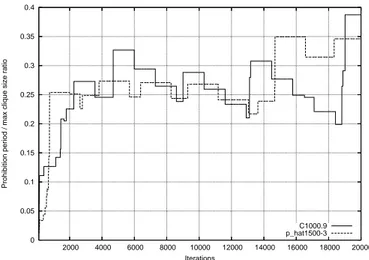
In Fig. 9 we show the evolution of T for a couple of
0 0.05 0.1 0.15 0.2 0.25 0.3 0.35 0.4 2000 4000 6000 8000 10000 12000 14000 16000 18000 20000
Prohibition period / max clique size ratio
Iterations
C1000.9 p_hat1500-3
Fig. 9. Dynamic evolution of the prohibition T (t) as a function of the iteration for runs onQbest.y-values are ratios between prohibition and best
clique sizeT (t)/Qbest(t).
55 60 65 70 75 80 85 90 95 0 0.2 0.4 0.6 0.8 1 1.2 1.4 1.6
Best clique found
Prohibition period to max clique ratio
p_hat1500-3 C1000.9
Fig. 10. FinalQbestresults obtained after a run of s-RLS (simplified RLS)
of 2000 iterations, as a function of theτ parameter. Error bars are at ±σ.
representative significant graphs. To make the approximate proportionality to the clique dimension clear we plot directly
the ratio between the currentT value and the size of the best
clique found at iterationt, called Qbest(t).
After confirming the hypothesis of a parameter T being
adapted to approximately a fraction of Qbest(t) we
exper-imented with a simplified reactive scheme which sets the
prohibition value T (t) equal to τ · Qbest(t). This version is
called a low-knowledge reactive scheme because the only information used from the previous history of the search is given by the size of the best clique.
The average results obtained forQbest in ten different runs
are plotted in Fig. 10. It can be observed that a small value
for the proportionality constant τ is associated to the best
results obtained. Furthermore, one observes a robust behavior
of the results as a function of τ , provided that its value
ranges approximately between 0.15 and 0.25. After these
experimental results, confirmed also on the other graphs, we
decided to fix τ = 0.2 for all cases.
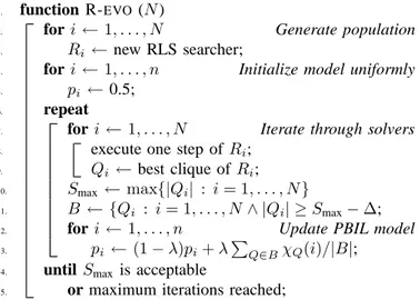
mech-1. function R-EVO(N )
2. fori ← 1, . . . , N Generate population 3. Ri ← new RLS searcher;
4. fori ← 1, . . . , n Initialize model uniformly 5. pi ← 0.5;
6. repeat
7. fori ← 1, . . . , N Iterate through solvers
8. execute one step ofRi;
9. Qi ← best clique of Ri; 10. Smax ← max{|Qi| : i = 1, . . . , N }
11. B ← {Qi : i = 1, . . . , N ∧ |Qi| ≥ Smax− ∆; 12. fori ← 1, . . . , n Update PBIL model 13. pi ← (1 − λ)pi+ λPQ∈BχQ(i)/|B|;
14. until Smax is acceptable
15. or maximum iterations reached;
Fig. 11. The RLS-EVOalgorithm for the Maximum Clique problem. The R-EVOsimplified version only differs in the implementation of the RLS step, so the pseudo-code fits R-EVOas well.
anism: the simplified version does not need to maintain a history structure, and the only action is to update the value ofT according to the size of the largest clique found up to
that moment.
IV. THE HYBRID EVOLUTIONARY AND REACTIVE
ALGORITHMS(R-EVO)
To distinguish the new and simplified version of RLS, the
hybrid algorithm is called R-EVO, while the hybrid algorithm
adopting the original RLS method is called RLS-EVO. Both
algorithms have the same overall structure, shown in Fig. 11.
The pool of searching individuals (Ri) is created with an
empty clique, and the initial estimate (pi) of the node
dis-tribution in the clique is set to a uniform value (each node
having a50% probability of appearing in a maximum clique).
Every iteration of the algorithm consists of a single iteration of each individual searcher (lines 7–9). After all searchers have been executed, the model is updated. The average is computed
by counting, for each node i, how many searchers include
nodei in their maximum clique. In order to reduce noise, only
searchers providing cliques whose size is comparable (within
a tolerance∆ ∈ N) with the largest one are taken into account.
The model(pi) is used within functionRestart(see the
RLS pseudo-code in Fig. 6) in order to build an initial clique with the most probable nodes. In detail, the initial clique is built in a greedy fashion, where candidate nodes at every step
are selected with probability proportional to model values(pi).
The model is the only data which is globally shared by all searchers.
V. COMPUTATIONAL EXPERIMENTS
All experiments have been performed with the following
parameters, derived from [13]: population ofN = 10
individ-uals, 10 runs per problem instance, model depth ∆ = 3; the
restart parameterA in Fig. 6 is 100 · Qbest. The EA/G data are
obtained from [13], where 20000 calls of the repair operator per run were considered. The construction of a new individual
in EA/G requires a sequence of node additions and removals,
while an R-EVO iteration only performs one node addition
or removal, so a direct comparison is not possible. To solve this problem, two series of experiments have been performed: one with a fixed but larger number of iterations, another with a number of iterations proportional to the maximum clique found. Both choices are motivated in the following sections.
Our experiments were executed on a Dual Xeon 3.4GHz machine with 6GB RAM and Linux 2.6 operating system. However, all tested algorithms were implemented as mono-lithic processes, so only a single processor core was in use at any time, and no CPU core parallelism has been exploited. To take hardware differences into account, some runs of EA/G have been reproduced and their average execution times were
used to obtain the 0.85 speedup factor used to re-estimate
execution times in the EA/G time columns.
A. Fixed number of iterations
The first series of tests was performed on R-EVO with
200, 000 solver steps (20, 000 steps per solver). The number
of iterations has been chosen in order to approach the amount of work that the EA/G heuristic performs at every iteration.
With this choice the execution times of R-EVOare significantly
lower than those allowed for EA/G, therefore the comparison is unbalanced in favor of EA/G.
Results are reported in Table I. The first set of columns reports the average maximum clique found (with the corre-sponding standard error), the overall maximum and the average execution time for 10 runs of the EA/G algorithm; the second set of columns contains the corresponding results for the
R-EVO algorithm. Finally, the results of a Student’s t-test for
equality of means with unequal sample variance [31] has been applied in order to test the equality of the two clique size averages (last column contains the significance of the null hypothesis, i.e., that the two distributions have the same average). Note that some tests could not be performed due to null variance in both algorithms.
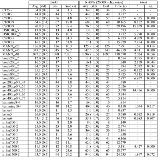
Results show that the R-EVO algorithm has a significant
superiority to EA/G in the case of dense random graphs (the
C*.9andDSJC*lines), for example the average size is7%
better in C2000.9; for the small instances both algorithms
always locate the maximum clique. The only gen*-type
in-stance (random graphs embedding a known clique) which was not always solved by both algorithms is the 400-node graph
with 55-node clique, where R-EVO outperforms EA/G. Also
the p_hat1500-* instances (random graphs with higher
spread in node degree) and thehamming*instances (graphs
of bit strings with connections between words if they are far
apart) show a slight superiority of R-EVOin the cases that are
not optimally solved by both algorithms.
The performance tends to be more difficult to assess in
the Brockington-Culberson graphs (thebrock*lines), where
the best clique is hidden in a very effective manner so that intelligent techniques tend to be not competitive with respect to brute force local search (in fact, the camouflaging process is designed to fool intelligent techniques).
The R-EVO algorithm does not perform at the EA/G level
TABLE I
COMPARISON BETWEENEA/GANDR-EVO FOR A FIXED NUMBER OF ITERATIONS.
EA/G R-EVO(200000) t-test
Avg. (std) Best Time (s) Avg. (std) Best Time (s) t sig.
C125.9 34.0 (0.0) 34 1.3 34.0 (0.0) 34 0.464 - -C250.9 44.0 (0.0) 44 2.5 44.0 (0.0) 44 0.491 - -C500.9 55.2 (0.9) 56 4.8 57.0 (0.0) 57 0.719 6.325 0.000 C1000.9 64.4 (1.4) 67 18.0 67.3 (0.5) 68 1.189 6.169 0.000 C2000.9 70.9 (1.0) 72 38.4 75.8 (0.6) 77 2.900 13.287 0.000 DSJC500 5 13.0 (0.0) 13 4.0 13.0 (0.0) 13 1.206 - -DSJC1000 5 14.5 (0.3) 15 10.3 15.0 (0.0) 15 3.107 5.270 0.000 C2000.5 14.9 (0.7) 16 24.3 16.0 (0.0) 16 4.372 4.969 0.001 C4000.5 16.1 (0.3) 17 51.9 17.0 (0.0) 17 9.342 9.487 0.000 MANN a27 126.0 (0.0) 126 10.3 125.6 (0.5) 126 0.651 2.530 0.026 MANN a45 343.7 (0.7) 345 68.2 342.2 (0.4) 343 2.852 5.883 0.000 MANN a81 1097.2 (0.6) 1098 705.1 1096.9 (0.6) 1098 5.754 1.118 0.208 brock200 2 12.0 (0.0) 12 1.5 11.5 (0.5) 12 0.844 3.162 0.009 brock200 4 16.5 (0.5) 17 1.7 16.1 (0.3) 17 0.500 2.169 0.044 brock400 2 24.7 (0.4) 25 3.1 25.0 (0.0) 25 0.722 2.372 0.034 brock400 4 25.1 (2.6) 33 3.3 25.8 (2.5) 33 1.158 0.614 0.323 brock800 2 20.1 (0.4) 21 7.6 21.0 (0.0) 21 1.430 7.115 0.000 brock800 4 19.9 (0.5) 21 7.6 21.0 (0.0) 21 2.253 6.957 0.000 gen200 p0.9 44 44.0 (0.0) 44 1.8 44.0 (0.0) 44 0.402 - -gen200 p0.9 55 55.0 (0.0) 55 3.3 55.0 (0.0) 55 0.586 - -gen400 p0.9 55 51.8 (0.7) 55 3.6 54.0 (1.1) 55 0.621 5.336 0.000 gen400 p0.9 65 65.0 (0.0) 65 3.6 65.0 (0.0) 65 0.940 - -gen400 p0.9 75 75.0 (0.0) 75 3.7 75.0 (0.0) 75 0.948 - -hamming8-4 16.0 (0.0) 16 1.7 16.0 (0.0) 16 0.597 - -hamming10-4 39.8 (0.6) 40 14.2 40.0 (0.0) 40 1.427 1.054 0.217 keller4 11.0 (0.0) 11 1.3 11.0 (0.0) 11 0.730 - -keller5 26.9 (0.3) 27 9.1 26.9 (0.3) 27 1.275 0.000 0.393 keller6 53.4 (1.2) 56 53.6 53.3 (0.7) 54 6.210 0.228 0.381 p hat300-1 8.0 (0.0) 8 2.0 8.0 (0.0) 8 1.191 - -p hat300-2 25.0 (0.0) 25 2.0 25.0 (0.0) 25 0.705 - -p hat300-3 36.0 (0.0) 36 2.3 36.0 (0.0) 36 0.972 - -p hat700-1 11.0 (0.0) 11 5.6 11.0 (0.0) 11 1.772 - -p hat700-2 44.0 (0.0) 44 7.6 44.0 (0.0) 44 1.407 - -p hat700-3 62.0 (0.0) 62 11.1 62.0 (0.0) 62 1.233 - -p hat1500-1 11.1 (0.3) 12 16.8 11.7 (0.5) 12 3.933 3.254 0.006 p hat1500-2 65.0 (0.0) 65 24.6 65.0 (0.0) 65 4.182 - -p hat1500-3 93.7 (0.5) 94 29.2 94.0 (0.0) 94 2.408 1.897 0.072
the t-test figures are uncertain in the larger case, where both techniques could find a (non-optimal, however) 1098-node clique. Finally, while average cliques are comparable in the
keller6instance, the 10 EA/G runs find a larger clique.
B. Iterations proportional to (estimated) maximum clique size
The CPU time differences in the previous series of ex-periments tended to increase on larger graphs, in particular on graphs with larger cliques. In order to attain a more fair comparison, we chose a different termination criterion
for R-EVO by limiting the overall number of iterations to
20, 000 × max{Qi}, where Qi is the maximum clique found
by searcherRi (see Fig. 11).
Results are reported on Table II. We can see that all cases where the null hypothesis is rejected with high confidence
(significance column< 0.05) R-EVOoutperforms EA/G, with
the exception of some Steiner Triple Problem (MANN*) and
Brockington-Culberson (brock*) instances. Note that time
differences have greatly reduced; in particular, now large graphs are searched for a time that is in the same order of magnitude as EA/G.
C. Internal comparison between R-EVOand RLS-EVO
Another set of experiments has been devoted to a
com-parison between the full-fledged RLS-EVO heuristic and its
much simpler low-knowledge R-EVOcounterpart used in the
previous experiments.
Results are shown in Table III. CPU times are not reported
because they are very similar in Table II for R-EVO. The
simpler version shows some marginal performance degrada-tion, but in many cases experimental variance is very large.
For instance, the more complex RLS-EVOfound the 33-node
clique of brock400_4once, and the higher average is due
to this single event.
The last group of columns in Table III refers to a final ex-periment with a mixed population: 5 searchers implement the
RLS-EVOalgorithms, 5 implement R-EVO. The results show
that in some cases this technique helps achieving the “best of both worlds,” however in other cases a slight degradation can
be observed. As examples, the brock400_4andkeller6
cases show that the mixed technique can obtain a performance equal to the best of its components.
TABLE II
COMPARISON BETWEENEA/GANDR-EVO FOR A NUMBER OF ITERATIONS PROPORTIONAL TO THE MAXIMUM DETECTED CLIQUE.
EA/G R-EVO(20000×cliquesize) t-test
Avg. (std) Best Time (s) Avg. (std) Best Time (s) t sig.
C125.9 34.0 (0.0) 34 1.3 34.0 (0.0) 34 1.215 - -C250.9 44.0 (0.0) 44 2.5 44.0 (0.0) 44 3.237 - -C500.9 55.2 (0.9) 56 4.8 57.0 (0.0) 57 4.227 6.325 0.000 C1000.9 64.4 (1.4) 67 18.0 68.0 (0.0) 68 10.165 8.132 0.000 C2000.9 70.9 (1.0) 72 38.4 76.5 (0.5) 77 29.196 15.839 0.000 DSJC500 5 13.0 (0.0) 13 4.0 13.0 (0.0) 13 1.573 - -DSJC1000 5 14.5 (0.3) 15 10.3 15.0 (0.0) 15 3.732 5.270 0.000 C2000.5 14.9 (0.7) 16 24.3 16.0 (0.0) 16 6.833 4.969 0.001 C4000.5 16.1 (0.3) 17 51.9 17.1 (0.3) 18 15.729 7.454 0.000 MANN a27 126.0 (0.0) 126 10.3 125.8 (0.4) 126 7.991 1.581 0.114 MANN a45 343.7 (0.7) 345 68.2 342.5 (0.5) 343 46.859 4.411 0.000 MANN a81 1097.2 (0.6) 1098 705.1 1096.7 (0.5) 1097 438.570 2.024 0.056 brock200 2 12.0 (0.0) 12 1.5 11.4 (0.5) 12 0.654 3.795 0.003 brock200 4 16.5 (0.5) 17 1.7 16.1 (0.3) 17 1.249 2.169 0.044 brock400 2 24.7 (0.4) 25 3.1 25.0 (0.0) 25 1.794 2.372 0.034 brock400 4 25.1 (2.6) 33 3.3 25.0 (0.0) 25 2.965 0.122 0.385 brock800 2 20.1 (0.4) 21 7.6 21.0 (0.0) 21 3.725 7.115 0.000 brock800 4 19.9 (0.5) 21 7.6 21.0 (0.0) 21 2.977 6.957 0.000 gen200 p0.9 44 44.0 (0.0) 44 1.8 44.0 (0.0) 44 1.789 - -gen200 p0.9 55 55.0 (0.0) 55 3.3 55.0 (0.0) 55 2.026 - -gen400 p0.9 55 51.8 (0.7) 55 3.6 55.0 (0.0) 55 3.378 14.456 0.000 gen400 p0.9 65 65.0 (0.0) 65 3.6 65.0 (0.0) 65 3.744 - -gen400 p0.9 75 75.0 (0.0) 75 3.7 75.0 (0.0) 75 5.114 - -hamming8-4 16.0 (0.0) 16 1.7 16.0 (0.0) 16 1.814 - -hamming10-4 39.8 (0.6) 40 14.2 40.0 (0.0) 40 8.110 1.054 0.217 keller4 11.0 (0.0) 11 1.3 11.0 (0.0) 11 0.837 - -keller5 26.9 (0.3) 27 9.1 26.8 (0.4) 27 3.680 0.632 0.319 keller6 53.4 (1.2) 56 53.6 53.7 (0.7) 55 34.573 0.683 0.307 p hat300-1 8.0 (0.0) 8 2.0 8.0 (0.0) 8 1.149 - -p hat300-2 25.0 (0.0) 25 2.0 25.0 (0.0) 25 2.774 - -p hat300-3 36.0 (0.0) 36 2.3 36.0 (0.0) 36 2.194 - -p hat700-1 11.0 (0.0) 11 5.6 11.0 (0.0) 11 1.950 - -p hat700-2 44.0 (0.0) 44 7.6 44.0 (0.0) 44 6.166 - -p hat700-3 62.0 (0.0) 62 11.1 62.0 (0.0) 62 12.579 - -p hat1500-1 11.1 (0.3) 12 16.8 11.8 (0.4) 12 5.181 4.427 0.000 p hat1500-2 65.0 (0.0) 65 24.6 65.0 (0.0) 65 18.577 - -p hat1500-3 93.7 (0.5) 94 29.2 94.0 (0.0) 94 24.735 1.897 0.072 VI. CONCLUSIONS
The paper presented a hybrid algorithm which uses an evolutionary scheme in the framework of “estimation of distribution algorithms” to generate new individuals, which are then subjected to memetic evolution through a simplified reactive search method. In this manner, each individual in the population executes a short local search with prohibition (a.k.a. tabu search). The prohibition period is determined in a simple reactive manner on a specific instance based on the estimated size of the maximum clique.
The results show that the proposed technique is competitive with respect to state-of-the-art evolutionary algorithms based on similar assumptions (the EA/G algorithm).
It is remarkable how a drastic simplification of the original RLS algorithm, complemented by the interaction of more pop-ulation members through a model derived by EDA is capable of achieving results which are comparable to those obtained by a very complex individual searcher. Coupling a limited form of “intelligence” (actually a low-knowledge reactive local search technique) with an evolutionary scheme achieves state-of-the-art results on the maximum clique problem.
ACKNOWLEDGMENT
The authors would like to thank Q. Zhang for sending the original software used in [13] and to acknowledge support by
F. Mascia for developing part of the R-EVOsoftware used in
the experimental part.
REFERENCES
[1] E. Marchiori, “A simple heuristic based genetic algorithm for the maximum clique problem,” Proceedings of the 1998 ACM symposium on Applied Computing, pp. 366–373, 1998.
[2] P. Moscato, “On evolution, search, optimization, genetic algorithms and martial arts: Towards memetic algorithms,” Caltech Concurrent Computation Program, Tech. Rep. C3P Report 826, 1989.
[3] P. Moscato and C. Cotta, “A gentle introduction to memetic algorithms,” Handbook of Metaheuristics, pp. 105–144, 2003.
[4] M. Clerc and J. Kennedy, “The particle swarm — explosion, stability, and convergence in a multidimensional complex space,” IEEE Transac-tions on Evolutionary Computation, vol. 6, no. 1, pp. 58–73, 2002. [5] S. Baluja, “Population-based incremental learning: A method for
in-tegrating genetic search based function optimization and competitive learning,” School of Comput. Sci., Carnegie Mellon University Pitts-burgh, PA, USA, Tech. Rep. CMU-CS-94-163, 1994.
[6] S. Baluja and R. Caruana, “Removing the genetics from the standard genetic algorithm,” School of Computer Science, Carnegie Mellon University, Tech. Rep. CMU-CS-95-141, 1995.
[7] H. M¨uhlenbein, “The equation for response to selection and its use for prediction,” Evolutionary Computation, vol. 5, no. 3, pp. 303–346, 1998.
TABLE III
INTERNAL COMPARISON BETWEEN A POPULATION OF10 R-EVO SEARCHERS,A POPULATION OF10 RLS-EVO SEARCHERS AND A MIXED POPULATION WITH5INDIVIDUALS OF EACH TYPE.
R-EVO RLS-EVO Mix
Avg. (std) Best Avg. (std) Best Avg. (std) Best
C125.9 34.0 (0.0) 34 34.0 (0.0) 34 34.0 (0.0) 34 C250.9 44.0 (0.0) 44 44.0 (0.0) 44 44.0 (0.0) 44 C500.9 57.0 (0.0) 57 57.0 (0.0) 57 57.0 (0.0) 57 C1000.9 68.0 (0.0) 68 67.9 (0.3) 68 67.9 (0.3) 68 C2000.9 76.5 (0.5) 77 76.2 (0.6) 77 76.2 (0.6) 77 DSJC500 5 13.0 (0.0) 13 13.0 (0.0) 13 13.0 (0.0) 13 DSJC1000 5 15.0 (0.0) 15 14.9 (0.3) 15 14.9 (0.3) 15 C2000.5 16.0 (0.0) 16 16.0 (0.0) 16 16.0 (0.0) 16 C4000.5 17.1 (0.3) 18 17.0 (0.0) 17 17.0 (0.0) 17 MANN a27 125.8 (0.4) 126 125.7 (0.5) 126 125.7 (0.5) 126 MANN a45 342.5 (0.5) 343 342.6 (0.5) 343 342.6 (0.5) 343 MANN a81 1096.7 (0.5) 1097 1097.0 (0.5) 1098 1097.0 (0.5) 1098 brock200 2 11.4 (0.5) 12 12.0 (0.0) 12 12.0 (0.0) 12 brock200 4 16.1 (0.3) 17 16.6 (0.5) 17 16.6 (0.5) 17 brock400 2 25.0 (0.0) 25 25.0 (0.0) 25 25.0 (0.0) 25 brock400 4 25.0 (0.0) 25 25.8 (2.5) 33 25.8 (2.5) 33 brock800 2 21.0 (0.0) 21 21.0 (0.0) 21 21.0 (0.0) 21 brock800 4 21.0 (0.0) 21 21.0 (0.0) 21 21.0 (0.0) 21 gen200 p0.9 44 44.0 (0.0) 44 44.0 (0.0) 44 44.0 (0.0) 44 gen200 p0.9 55 55.0 (0.0) 55 55.0 (0.0) 55 55.0 (0.0) 55 gen400 p0.9 55 55.0 (0.0) 55 55.0 (0.0) 55 55.0 (0.0) 55 gen400 p0.9 65 65.0 (0.0) 65 65.0 (0.0) 65 65.0 (0.0) 65 gen400 p0.9 75 75.0 (0.0) 75 75.0 (0.0) 75 75.0 (0.0) 75 hamming8-4 16.0 (0.0) 16 16.0 (0.0) 16 16.0 (0.0) 16 hamming10-4 40.0 (0.0) 40 40.0 (0.0) 40 40.0 (0.0) 40 keller4 11.0 (0.0) 11 11.0 (0.0) 11 11.0 (0.0) 11 keller5 26.8 (0.4) 27 27.0 (0.0) 27 27.0 (0.0) 27 keller6 53.7 (0.7) 55 59.0 (0.0) 59 59.0 (0.0) 59 p hat300-1 8.0 (0.0) 8 8.0 (0.0) 8 8.0 (0.0) 8 p hat300-2 25.0 (0.0) 25 25.0 (0.0) 25 25.0 (0.0) 25 p hat300-3 36.0 (0.0) 36 36.0 (0.0) 36 36.0 (0.0) 36 p hat700-1 11.0 (0.0) 11 11.0 (0.0) 11 11.0 (0.0) 11 p hat700-2 44.0 (0.0) 44 44.0 (0.0) 44 44.0 (0.0) 44 p hat700-3 62.0 (0.0) 62 62.0 (0.0) 62 62.0 (0.0) 62 p hat1500-1 11.8 (0.4) 12 11.6 (0.5) 12 11.6 (0.5) 12 p hat1500-2 65.0 (0.0) 65 65.0 (0.0) 65 65.0 (0.0) 65 p hat1500-3 94.0 (0.0) 94 94.0 (0.0) 94 94.0 (0.0) 94
[8] M. Pelikan, D. Goldberg, and E. Cantu-Paz, “Boa: The bayesian optimization algorithm,” Proceedings of the Genetic and Evolutionary Computation Conference GECCO-99, vol. 1, pp. 525–532, 1999. [9] P. Larranaga, Estimation of Distribution Algorithms: A New Tool for
Evolutionary Computation. Kluwer Academic Publishers, 2001. [10] F. Glover, “Scatter search and star-paths: beyond the genetic metaphor,”
Operations Research Spektrum, vol. 17, no. 2/3, pp. 125–138, 1995. [11] F. Glover, M. Laguna, and R. Mart´ı, “Scatter search,” in Advances
in Evolutionary Computation: Theory and Applications, A. Ghosh and S. Tsutsui, Eds. Springer-Verlag, New York, 2003, pp. 519–537. [12] F. Glover, “Tabu search — part I,” ORSA Journal on Computing, vol. 1,
no. 3, pp. 190–260, 1989.
[13] Q. Zhang, J. Sun, and E. Tsang, “An evolutionary algorithm with guided mutation for the maximum clique problem,” IEEE Transactions on Evolutionary Computation, vol. 9, no. 2, pp. 192–200, 2005. [14] E. Marchiori, “Genetic, iterated and multistart local search for the
maximum clique problem,” Applications of Evolutionary Computing, vol. 2279, pp. 112–121, 2002.
[15] J. S. de Bonet, C. L. I. Jr., and P. Viola, “MIMIC: Finding optima by estimating probability densities,” in Advances in Neural Information Processing Systems, M. C. Mozer, M. I. Jordan, and T. Petsche, Eds., vol. 9. The MIT Press, 1997, p. 424.
[16] P. Pardalos and J. Xue, “The maximum clique problem,” Journal of Global Optimization, vol. 4, pp. 301–328, 1994.
[17] Y. Ji, X. Xu, and G. Stormo, “A graph theoretical approach to pre-dict common rna secondary structure motifs including pseudoknots in unaligned sequences,” Bioinformatics, vol. 20, no. 10, pp. 1591–1602, 2004.
[18] S. Butenko and W. Wilhelm, “Clique-detection models in
computa-tional biochemistry and genomics,” European Journal of Operacomputa-tional Research, 2006, to appear.
[19] J. H˚astad, “Clique is hard to approximate withinn1−ǫ,” in Proc. 37th
Ann. IEEE Symp. on Foundations of Computer Science. IEEE Computer Society, 1996, pp. 627–636.
[20] R. Battiti and M. Protasi, “Reactive local search for the maximum clique problem,” Algorithmica, vol. 29, no. 4, pp. 610–637, 2001.
[21] R. Battiti, M. Brunato, and F. Mascia, Reactive Search and Intelli-gent Optimization. Via Sommarive 14, 38100, Trento - Italy: DIT - University of Trento, Apr. 2007, available at http://www.reactive-search.org/thebook/.
[22] R. Battiti and G. Tecchiolli, “The reactive tabu search,” ORSA Journal on Computing, vol. 6, no. 2, pp. 126–140, 1994.
[23] R. Battiti and A. A. Bertossi, “Greedy, prohibition, and reactive heuris-tics for graph partitioning,” IEEE Transactions on Computers, vol. 48, no. 4, pp. 361–385, Apr. 1999.
[24] H. M¨uhlenbein and G. Paaß, “From recombination of genes to the estimation of distributions i. binary parameters,” in Parallel Problem Solving from Nature — PPSN IV, A. Eiben, T. B¨ack, M. Schoenauer, and H. Schwefel, Eds., 1996, pp. 178–187.
[25] M. Pelikan, D. Goldberg, and F. Lobo, “A survey of optimization by building and using probabilistic models,” Computational Optimization and Applications, vol. 21, no. 1, pp. 5–20, 2002.
[26] M. Zlochin, M. Birattari, N. Meuleau, and M. Dorigo, “Model-based search for combinatorial optimization,” Annals of Operations Research, no. 131, pp. 373–395, 2004.
[27] J. Hertz, A. Krogh, and R. Palmer, Introduction to the Theory of Neural Computation. Redwood City, CA: Addison-Wesley Publishing Company, Inc., 1991.
[29] R. Battiti and M. Protasi, “Reactive local search for the maximum clique problem,” ICSI, 1947 Center St.- Suite 600 - Berkeley, California, Tech. Rep. TR-95-052, Sep 1995.
[30] R. Battiti and F. Mascia, “Reactive local search for maximum clique: a new implementation,” University of Trento, Tech. Rep. DIT-07-018, 2007.
[31] W. H. Press, B. P. Flannery, S. A. Teukolsky, and W. T. Vetterling, Numerical Recipes in C, 2nd ed. Cambridge University Press, 1992.